A Semi-Automated Method to Extract Green and Non-Photosynthetic Vegetation Cover from RGB Images in Mixed Grasslands


Abstract
1. Introduction
2. Materials and Methods
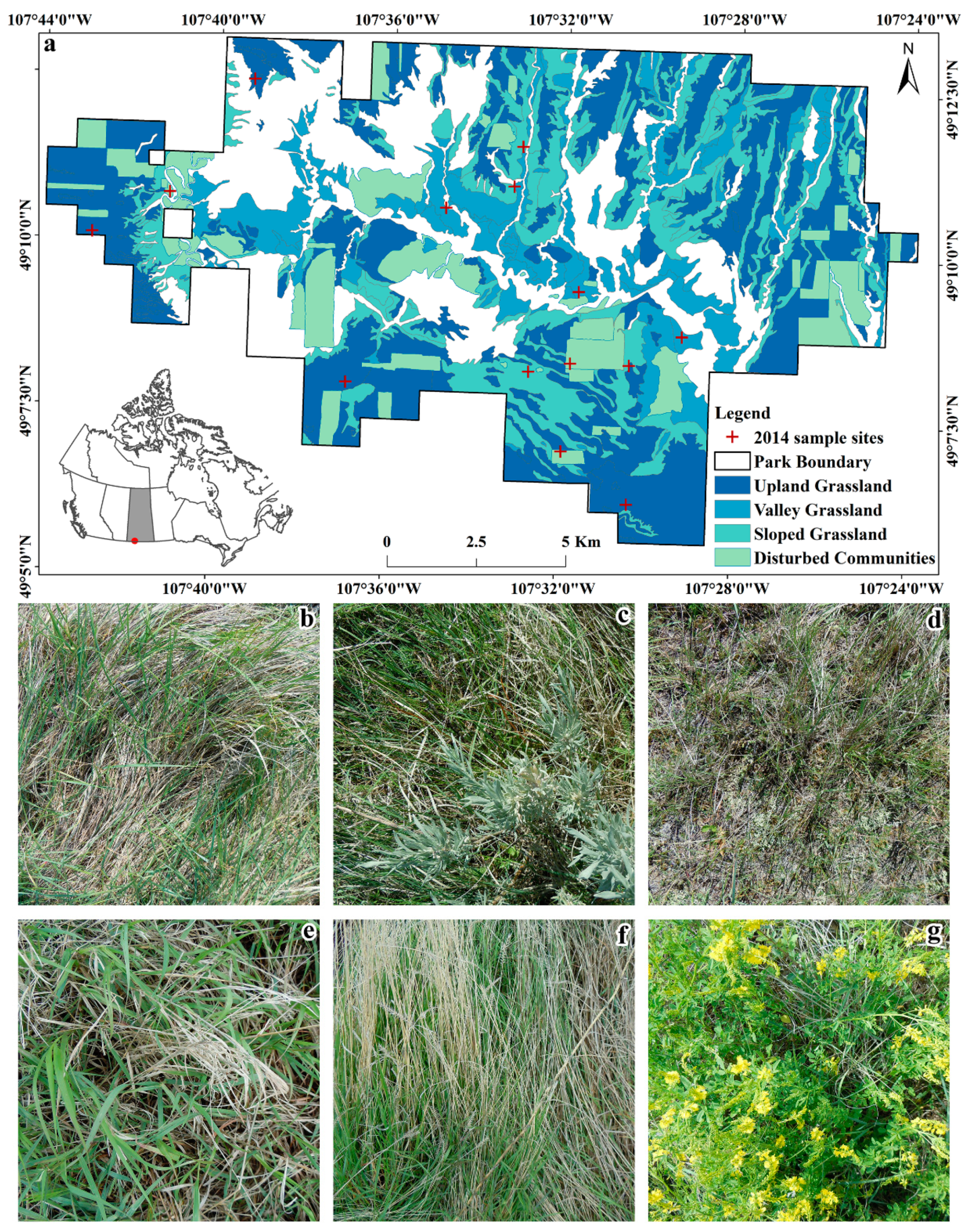
2.1. Study Area
2.2. Field Data Collection
2.3. Methods
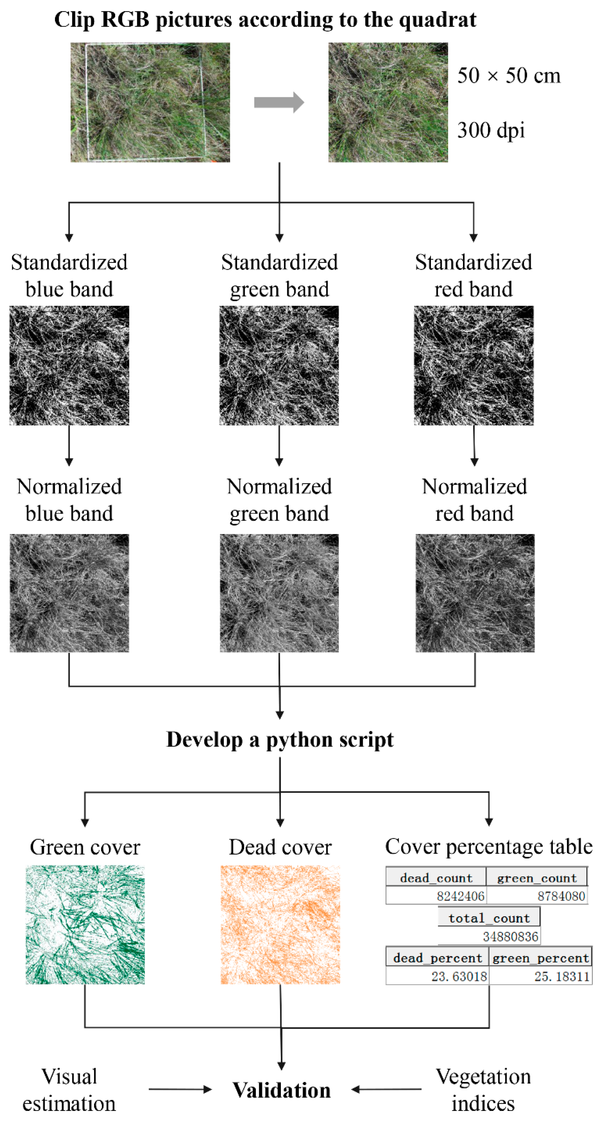
2.3.1. Pre-Processing for the Field-Taken RGB Images
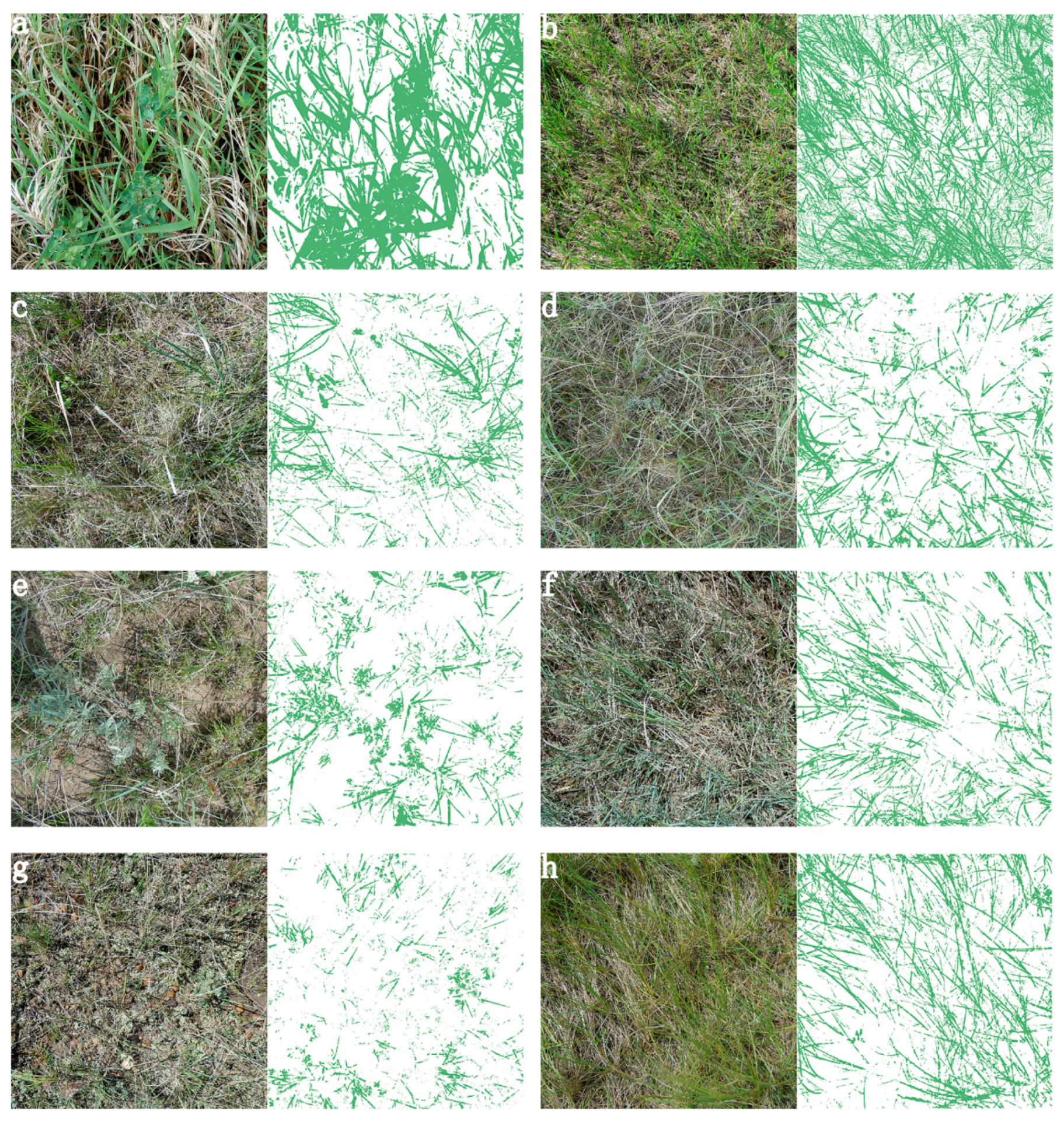
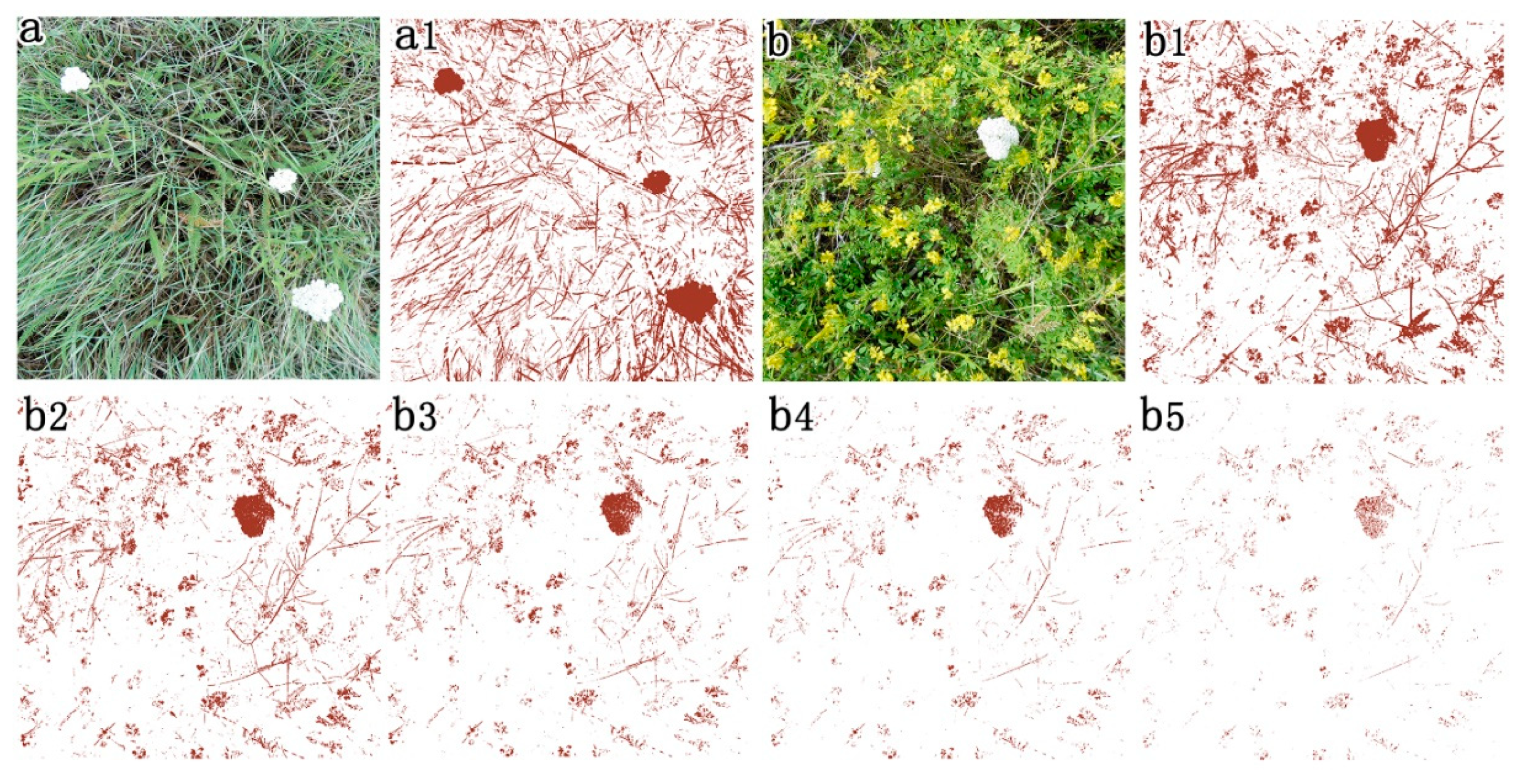
2.3.2. Developing a Python Script to Semi-Automate GV and SDM Cover Extraction from Preprocessed RGB Images
2.3.3. Validation of Extracted GV and SDM Cover from RGB Images
3. Results
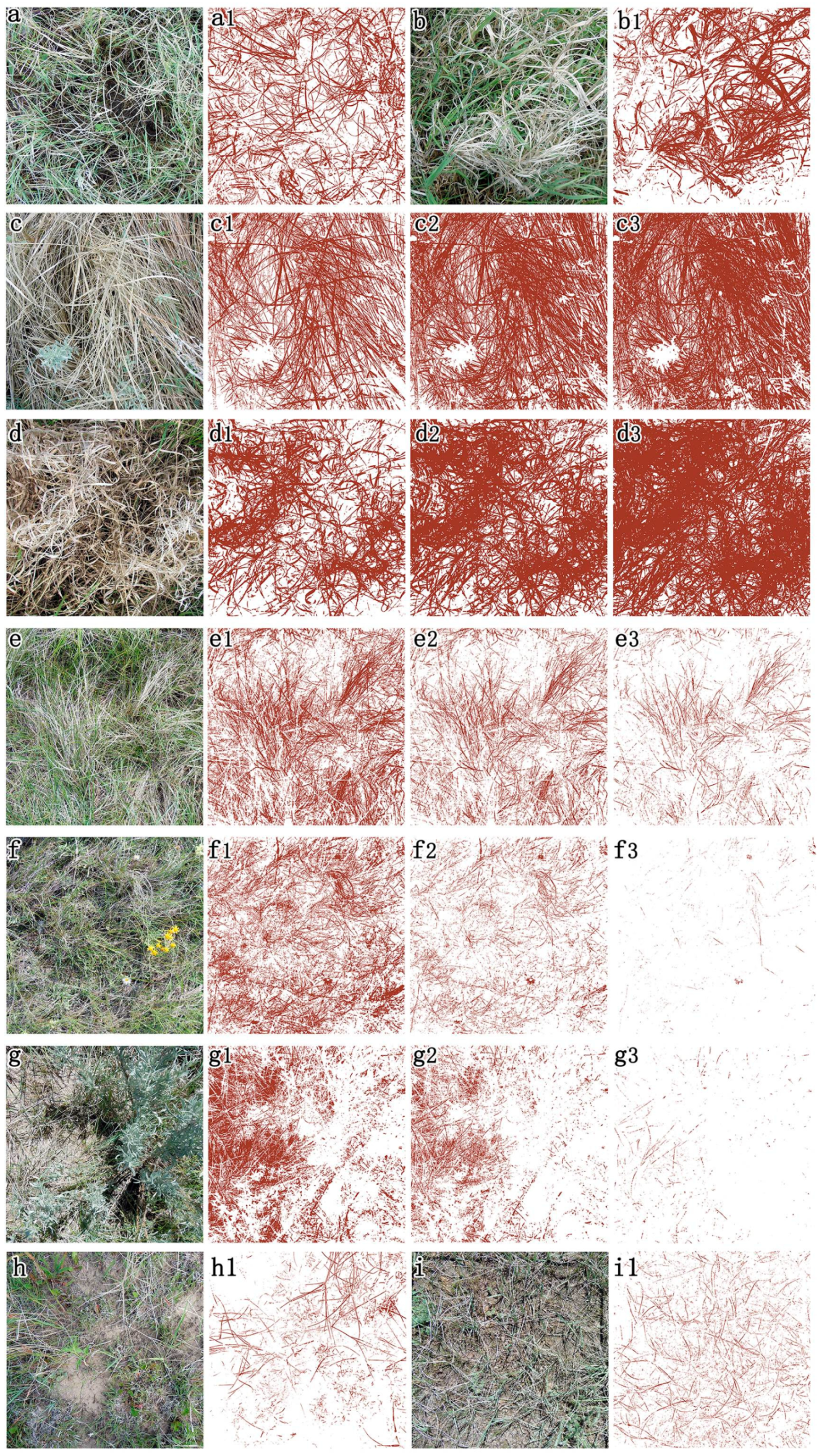
3.1. Determination of the Constants for GV Extraction
3.2. Setting of the Constant for SDM Extraction
3.3. GV and SDM Cover Estimated from RGB Images
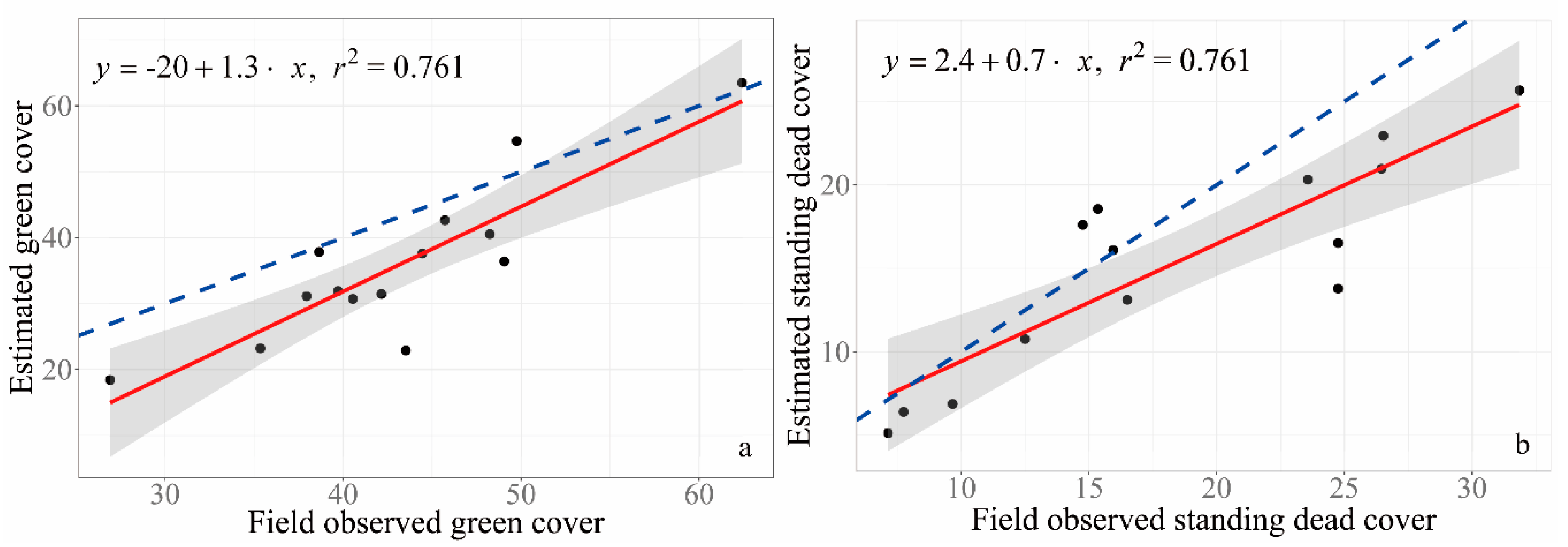
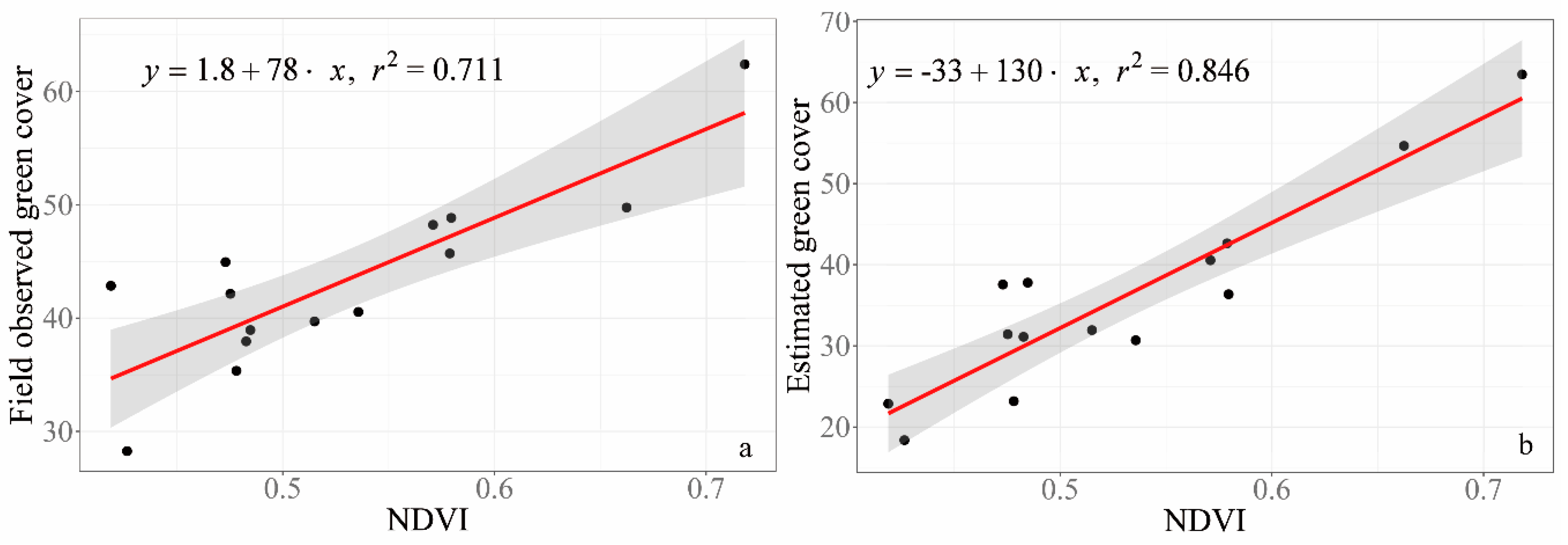
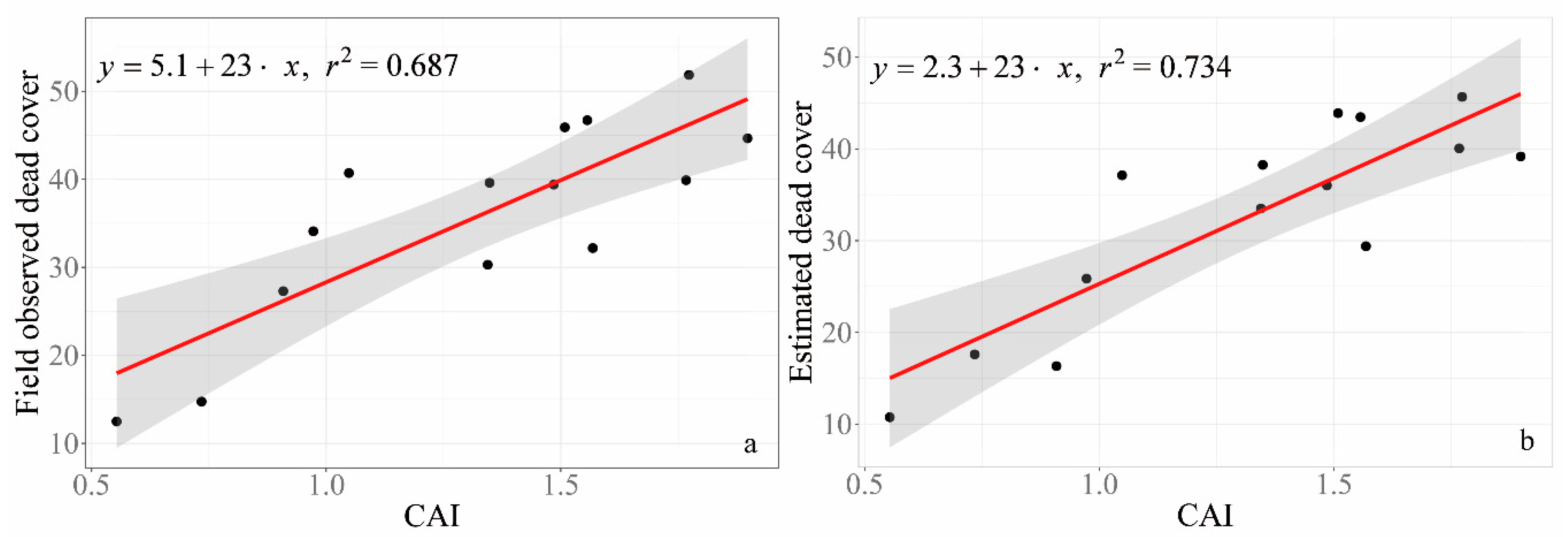
3.4. Validation of GV and NPV Estimated from RGB Images
4. Discussion
4.1. GV and SDM Cover Estimation Based on RGB Images and Visual Estimation
4.2. Estimated Green Cover from RGB Pictures
4.3. Estimated SDM from RGB Images
5. Conclusions
Supplementary Materials
Author Contributions
Funding
Acknowledgments
Conflicts of Interest
References
- Liu, Y.; Mu, X.; Wang, H.; Yan, G. A novel method for extracting green fractional vegetation cover from digital images. J. Veg. Sci. 2011, 23, 406–418. [Google Scholar] [CrossRef]
- Lee, K.J.; Lee, B.-W. Estimating canopy cover from color digital camera image of rice field. J. Crop. Sci. Biotechnol. 2011, 14, 151–155. [Google Scholar] [CrossRef]
- Hu, J.; Dai, M.X.; Peng, S.T. An automated (novel) algorithm for estimating green vegetation cover fraction from digital image: UIP-MGMEP. Environ. Monit. Assess. 2018, 190, 687. [Google Scholar] [CrossRef]
- Zhao, C.; Li, C.; Wang, Q.; Meng, Q.; Wang, J. Automated Digital Image Analyses For Estimating Percent Ground Cover of Winter Wheat Based on Object Features. In International Conference on Computer and Computing Technologies in Agriculture; Li, D., Zhao, C., Eds.; Springer Science and Business Media LLC: Boston, MA, USA, 2009; Volume 293, pp. 253–264. [Google Scholar]
- Luscier, J.D.; Thompson, W.L.; Wilson, J.M.; Gorham, B.E.; Dragut, L.D. Using digital photographs and object-based image analysis to estimate percent ground cover in vegetation plots. Front. Ecol. Environ. 2006, 4, 408–413. [Google Scholar] [CrossRef]
- Song, W.; Mu, X.; Yan, G.; Huang, S. Extracting the Green Fractional Vegetation Cover from Digital Images Using a Shadow-Resistant Algorithm (SHAR-LABFVC). Remote Sens. 2015, 7, 10425–10443. [Google Scholar] [CrossRef]
- Büchi, L.; Wendling, M.; Mouly, P.; Charles, R. Comparison of Visual Assessment and Digital Image Analysis for Canopy Cover Estimation. Agron. J. 2018, 110, 1289–1295. [Google Scholar] [CrossRef]
- Olmstead, M.A.; Wample, R.; Greene, S.; Tarara, J. Nondestructive Measurement of Vegetative Cover Using Digital Image Analysis. HortScience 2004, 39, 55–59. [Google Scholar] [CrossRef]
- Baxendale, C.; Ostle, N.J.; Wood, C.M.; Oakley, S.; Ward, S.E.; Ostle, N.J. Can digital image classification be used as a standardised method for surveying peatland vegetation cover? Ecol. Indic. 2016, 68, 150–156. [Google Scholar] [CrossRef]
- Kim, J.; Kang, S.; Seo, B.; Narantsetseg, A.; Han, Y.-J. Estimating fractional green vegetation cover of Mongolian grasslands using digital camera images and MODIS satellite vegetation indices. GIScience Remote Sens. 2019, 57, 49–59. [Google Scholar] [CrossRef]
- Xiong, Y.; West, C.P.; Brown, C.; Green, P. Digital Image Analysis of Old World Bluestem Cover to Estimate Canopy Development. Agron. J. 2019, 111, 1247–1253. [Google Scholar] [CrossRef]
- Zhou, Q.; Robson, M. Automated rangeland vegetation cover and density estimation using ground digital images and a spectral-contextual classifier. Int. J. Remote Sens. 2001, 22, 3457–3470. [Google Scholar] [CrossRef]
- Xu, D.; Guo, X.; Li, Z.; Yang, X.; Yin, H. Measuring the dead component of mixed grassland with Landsat imagery. Remote Sens. Environ. 2014, 142, 33–43. [Google Scholar] [CrossRef]
- Makanza, R.; Zaman-Allah, M.; Cairns, J.E.; Magorokosho, C.; Tarekegne, A.; Olsen, M.; Prasanna, B.M. High-Throughput Phenotyping of Canopy Cover and Senescence in Maize Field Trials Using Aerial Digital Canopy Imaging. Remote Sens. 2018, 10, 330. [Google Scholar] [CrossRef]
- Lynch, T.M.H.; Barth, S.; Dix, P.J.; Grogan, D.; Grant, J.; Grant, O.M. Ground Cover Assessment of Perennial Ryegrass Using Digital Imaging. Agron. J. 2015, 107, 2347–2352. [Google Scholar] [CrossRef]
- Macfarlane, C.; Ogden, G.N. Automated estimation of foliage cover in forest understorey from digital nadir images. Methods Ecol. Evol. 2011, 3, 405–415. [Google Scholar] [CrossRef]
- Chianucci, F.; Chiavetta, U.; Cutini, A. The estimation of canopy attributes from digital cover photography by two different image analysis methods. iForest-Biogeosciences For. 2014, 7, 255–259. [Google Scholar] [CrossRef]
- Alivernini, A.; Fares, S.; Ferrara, C.; Chianucci, F. An objective image analysis method for estimation of canopy attributes from digital cover photography. Trees-Struct. Funct. 2018, 32, 713–723. [Google Scholar] [CrossRef]
- Marcial-Pablo, M.D.J.; Gonzalez-Sanchez, A.; Jimenez-Jimenez, S.I.; Ontiveros-Capurata, R.E.; Ojeda-Bustamante, W. Estimation of vegetation fraction using RGB and multispectral images from UAV. Int. J. Remote Sens. 2019, 40, 420–438. [Google Scholar] [CrossRef]
- Bin Zhang, Z.; Liu, C.X.; Xu, X.D. A Green Vegetation Extraction Based-RGB Space in Natural Sunlight. Adv. Mater. Res. 2011, 660–665. [Google Scholar] [CrossRef]
- Chen, A.; Orlov-Levin, V.; Meron, M. Applying high-resolution visible-channel aerial imaging of crop canopy to precision irrigation management. Agric. Water Manag. 2019, 216, 196–205. [Google Scholar] [CrossRef]
- Comar, A.; Burger, P.; De Solan, B.; Baret, F.; Daumard, F.; Hanocq, J.-F. A semi-automatic system for high throughput phenotyping wheat cultivars in-field conditions: Description and first results. Funct. Plant Biol. 2012, 39, 914–924. [Google Scholar] [CrossRef] [PubMed]
- Velázquez-García, J.; Oleschko, K.; Muñoz-Villalobos, J.A.; Velásquez-Valle, M.; Menes, M.M.; Parrot, J.-F.; Korvin, G.; Cerca, M. Land cover monitoring by fractal analysis of digital images. Geoderma 2010, 160, 83–92. [Google Scholar] [CrossRef]
- Liu, N.; Treitz, P. Modelling high arctic percent vegetation cover using field digital images and high resolution satellite data. Int. J. Appl. Earth Obs. Geoinf. 2016, 52, 445–456. [Google Scholar] [CrossRef]
- Fuentes-Peailillo, F.; Ortega-Farias, S.; Rivera, M.; Bardeen, M.; Moreno, M. Comparison of vegetation indices acquired from RGB and Multispectral sensors placed on UAV. In Proceedings of the 2018 IEEE International Conference on Automation/XXIII Congress of the Chilean Association of Automatic Control (ICA-ACCA), Concepcion, Chile, 17–19 October 2018; Institute of Electrical and Electronics Engineers (IEEE): New York, NY, USA, 2018; pp. 1–6. [Google Scholar]
- Roth, L.; Aasen, H.; Walter, A.; Liebisch, F. Extracting leaf area index using viewing geometry effects—A new perspective on high-resolution unmanned aerial system photography. ISPRS J. Photogramm. Remote Sens. 2018, 141, 161–175. [Google Scholar] [CrossRef]
- Laliberte, A.; Rango, A.; Herrick, J.; Fredrickson, E.L.; Burkett, L. An object-based image analysis approach for determining fractional cover of senescent and green vegetation with digital plot photography. J. Arid. Environ. 2007, 69, 1–14. [Google Scholar] [CrossRef]
- Booth, D.T.; Cox, S.E.; Berryman, R.D. Point Sampling Digital Imagery with ‘Samplepoint’. Environ. Monit. Assess. 2006, 123, 97–108. [Google Scholar] [CrossRef]
- Mora, M.; Ávila, F.; Carrasco-Benavides, M.; Maldonado, G.; Olguín-Cáceres, J.; Fuentes, S. Automated computation of leaf area index from fruit trees using improved image processing algorithms applied to canopy cover digital photograpies. Comput. Electron. Agric. 2016, 123, 195–202. [Google Scholar] [CrossRef]
- Xu, D.; Guo, X. A Study of Soil Line Simulation from Landsat Images in Mixed Grassland. Remote Sens. 2013, 5, 4533–4550. [Google Scholar] [CrossRef]
- Rasmussen, J.; Nørremark, M.; Bibby, B. Assessment of leaf cover and crop soil cover in weed harrowing research using digital images. Weed Res. 2007, 47, 299–310. [Google Scholar] [CrossRef]
- Nagler, P.L.; Inoue, Y.; Glenn, E.; Russ, A.; Daughtry, C.S.T. Cellulose absorption index (CAI) to quantify mixed soil–plant litter scenes. Remote Sens. Environ. 2003, 87, 310–325. [Google Scholar] [CrossRef]
- Ren, H.; Zhou, G.; Zhang, F.; Zhang, X. Evaluating cellulose absorption index (CAI) for non-photosynthetic biomass estimation in the desert steppe of Inner Mongolia. Chin. Sci. Bull. 2012, 57, 1716–1722. [Google Scholar] [CrossRef]
- Aguilar, J.; Evans, R.; Daughtry, C.S.T. Performance assessment of the cellulose absorption index method for estimating crop residue cover. J. Soil Water Conserv. 2012, 67, 202–210. [Google Scholar] [CrossRef]
- Richardson, M.D.; Karcher, D.E.; Purcell, L.C. Quantifying Turfgrass Cover Using Digital Image Analysis. Crop. Sci. 2001, 41, 1884–1888. [Google Scholar] [CrossRef]
- Patrignani, A.; Ochsner, T.E. Canopeo: A Powerful New Tool for Measuring Fractional Green Canopy Cover. Agron. J. 2015, 107, 2312–2320. [Google Scholar] [CrossRef]


| Vegetation Community | Dominated Species |
|---|---|
| upland grassland | western wheatgrass (Agropyron smithii Rydb.) |
| blue grama grass (Bouteloua gracilis (HBK) Lang. ex Steud.) | |
| needle-and-thread grass (Stipa comata Trin. and Rupr.) | |
| valley grassland | northern wheatgrass (Agropyron dasystachym) |
| western wheatgrass (Agropyron smithii Rydb.) | |
| with high density of shrub species | |
| sloped grassland | northern wheatgrass (Agropyron dasystachym) |
| western wheatgrass (Agropyron smithii Rydb.) | |
| needle-and-thread grass (Stipa comata Trin. and Rupr.) | |
| blue grama grass (Bouteloua gracilis (HBK) Lang. ex Steud.) | |
| disturbed communities | crested wheatgrass (Agropyron cristatum) |
| smooth brome (Bromus inermis Layss.) | |
| sweet clover (Melilotus officinalis) |
| ID | Vegetation Community | Green Cover (GV) | Standing Dead Matter (SDM) Cover | Non-Photosynthetic Vegetation (NPV) Cover | |||
|---|---|---|---|---|---|---|---|
| Mean | Standard Deviation (STD) | Mean | STD | Mean | STD | ||
| 1 | upland grassland | 48.85 | 13.02 | 7.75 | 8.50 | 39.60 | 8.77 |
| 2 | upland grassland | 42.15 | 14.72 | 31.85 | 9.18 | 51.85 | 11.89 |
| 3 | upland grassland | 48.24 | 6.91 | 7.14 | 5.82 | 45.90 | 6.36 |
| 4 | upland grassland | 40.55 | 9.61 | 16.50 | 9.75 | 39.40 | 19.37 |
| 5 | valley grassland | 42.85 | 14.04 | 24.75 | 11.97 | 27.30 | 12.21 |
| 6 | valley grassland | 37.95 | 12.39 | 24.75 | 11.53 | 34.10 | 14.97 |
| 7 | valley grassland | 45.71 | 16.30 | 26.52 | 18.90 | 40.71 | 20.08 |
| 8 | sloped grassland | 28.25 | 13.35 | 15.35 | 16.33 | 30.30 | 22.66 |
| 9 | sloped grassland | 35.35 | 10.92 | 26.45 | 14.33 | 44.65 | 20.05 |
| 10 | sloped grassland | 39.71 | 10.62 | 23.57 | 14.24 | 46.71 | 12.36 |
| 11 | sloped grassland | 44.95 | 7.35 | 15.95 | 8.75 | 39.90 | 11.71 |
| 12 | sloped grassland | 38.95 | 8.96 | 9.67 | 5.18 | 32.19 | 11.60 |
| 13 | disturbed communities | 62.40 | 18.86 | 12.50 | 7.86 | 12.50 | 7.86 |
| 14 | disturbed communities | 49.76 | 11.34 | 14.76 | 10.30 | 14.76 | 10.30 |
| ID | Vegetation Community | Species | Condition | g1 | g2 | ||||||
|---|---|---|---|---|---|---|---|---|---|---|---|
| MIN | MAX | MEAN | STD | MIN | MAX | MEAN | STD | ||||
| 1 | disturbed community | smooth brome/forb | normal condition | 60.18 | 276.81 | 139.94 | 41.26 | 60.53 | 533.56 | 199.87 | 60.55 |
| 2 | disturbed community | smooth brome | normal condition | 60.23 | 268.79 | 133.36 | 38.97 | 60.24 | 517.52 | 192.35 | 65.15 |
| 3 | disturbed community | smooth brome/forb | normal condition | 60.18 | 260.76 | 124.73 | 36.37 | 60.33 | 577.69 | 226.32 | 67.68 |
| 4 | disturbed community | smooth brome | high exposure | 38.12 | 224.66 | 94.36 | 23.41 | 60.15 | 545.60 | 267.27 | 55.50 |
| 5 | disturbed community | sweet clover | normal condition | 64.22 | 649.91 | 198.42 | 74.89 | 66.13 | 1014.98 | 434.55 | 167.75 |
| 6 | disturbed community | sweet clover | normal condition | 64.11 | 328.96 | 170.97 | 51.25 | 66.03 | 776.71 | 333.94 | 98.38 |
| 7 | sloped grassland | needle and thread/northern wheat grass | high exposure | 32.09 | 577.69 | 119.27 | 50.33 | 60.47 | 774.27 | 201.43 | 83.10 |
| 8 | sloped grassland | western wheat grass/needle and thread | high exposure | 36.11 | 284.84 | 106.99 | 33.44 | 60.36 | 585.72 | 147.92 | 59.82 |
| 9 | sloped grassland | needle and thread | senesced grass | 40.12 | 196.58 | 79.25 | 18.26 | 60.33 | 469.38 | 180.69 | 63.62 |
| 10 | sloped grassland | needle and thread/western wheat grass | high exposure | 44.13 | 517.52 | 117.68 | 50.47 | 60.23 | 786.31 | 248.96 | 85.93 |
| 11 | sloped grassland | June grass/needle and thread/forb | high exposure, senesced grass | 44.13 | 244.72 | 96.79 | 27.01 | 60.34 | 625.84 | 256.16 | 81.21 |
| 12 | sloped grassland | June grass/western wheat grass | normal condition | 61.02 | 284.84 | 117.41 | 38.13 | 60.15 | 501.47 | 155.81 | 60.03 |
| 13 | sloped grassland | June grass/western wheat grass | normal condition | 60.39 | 280.82 | 129.48 | 41.20 | 61.11 | 509.49 | 165.86 | 63.25 |
| 14 | sloped grassland | June grass/western wheat grass/forb | normal condition | 61.54 | 252.74 | 106.01 | 33.76 | 60.02 | 469.38 | 132.68 | 54.99 |
| 15 | upland grassland | northern wheat grass | high exposure, senesced grass | 36.11 | 445.31 | 127.37 | 50.69 | 60.03 | 710.47 | 299.97 | 83.84 |
| 16 | upland grassland | June grass/northern wheat grass | senesced grass | 40.12 | 296.87 | 108.04 | 34.27 | 62.11 | 585.72 | 185.94 | 77.32 |
| 17 | upland grassland | northern wheat grass/needle and thread | high exposure, senesced grass | 36.11 | 240.71 | 100.90 | 28.54 | 63.12 | 557.64 | 264.67 | 60.56 |
| 18 | upland grassland | western wheat grass/needle and thread | normal condition | 61.27 | 629.85 | 132.76 | 55.72 | 60.01 | 826.42 | 281.67 | 96.35 |
| 19 | valley grassland | western wheat grass | bluish leaves | 61.22 | 224.66 | 86.35 | 22.01 | 32.09 | 453.33 | 120.11 | 43.96 |
| 20 | valley grassland | crested wheat grass | bluish leaves | 60.14 | 260.76 | 116.32 | 34.09 | 36.11 | 561.65 | 199.28 | 74.63 |
| 21 | valley grassland | western wheat grass/sagebrush | bluish leaves | 60.18 | 256.75 | 95.04 | 25.59 | 40.12 | 533.56 | 157.27 | 65.15 |
| 22 | valley grassland | smooth brome/forb | normal condition | 66.13 | 300.88 | 162.84 | 47.67 | 64.19 | 429.26 | 177.65 | 55.57 |
| 23 | valley grassland | northern wheat grass | normal condition | 61.22 | 276.81 | 114.85 | 36.49 | 60.23 | 485.42 | 137.31 | 55.02 |
| 24 | valley grassland | western wheat grass/Little blue steam | normal condition | 62.12 | 216.64 | 90.98 | 23.61 | 60.01 | 477.40 | 168.68 | 51.78 |
| 25 | valley grassland | western wheat grass/forb | bluish leaves | 60.28 | 232.68 | 90.59 | 22.40 | 40.12 | 272.80 | 125.49 | 41.29 |
Publisher’s Note: MDPI stays neutral with regard to jurisdictional claims in published maps and institutional affiliations. |
© 2020 by the authors. Licensee MDPI, Basel, Switzerland. This article is an open access article distributed under the terms and conditions of the Creative Commons Attribution (CC BY) license (http://creativecommons.org/licenses/by/4.0/).
Share and Cite
Xu, D.; Pu, Y.; Guo, X. A Semi-Automated Method to Extract Green and Non-Photosynthetic Vegetation Cover from RGB Images in Mixed Grasslands. Sensors 2020, 20, 6870. https://doi.org/10.3390/s20236870
Xu D, Pu Y, Guo X. A Semi-Automated Method to Extract Green and Non-Photosynthetic Vegetation Cover from RGB Images in Mixed Grasslands. Sensors. 2020; 20(23):6870. https://doi.org/10.3390/s20236870
Chicago/Turabian StyleXu, Dandan, Yihan Pu, and Xulin Guo. 2020. "A Semi-Automated Method to Extract Green and Non-Photosynthetic Vegetation Cover from RGB Images in Mixed Grasslands" Sensors 20, no. 23: 6870. https://doi.org/10.3390/s20236870
APA StyleXu, D., Pu, Y., & Guo, X. (2020). A Semi-Automated Method to Extract Green and Non-Photosynthetic Vegetation Cover from RGB Images in Mixed Grasslands. Sensors, 20(23), 6870. https://doi.org/10.3390/s20236870