Dimensioning Method of Floating Offshore Objects by Means of Quasi-Similarity Transformation with Reduced Tolerance Errors


Abstract
1. Introduction
- —translation vector,
- —vector (point) in the original system (subject to transformation),
- —vector (point) in the secondary system (treated as stationary),
- —scale factor,
- R—rotation matrix.
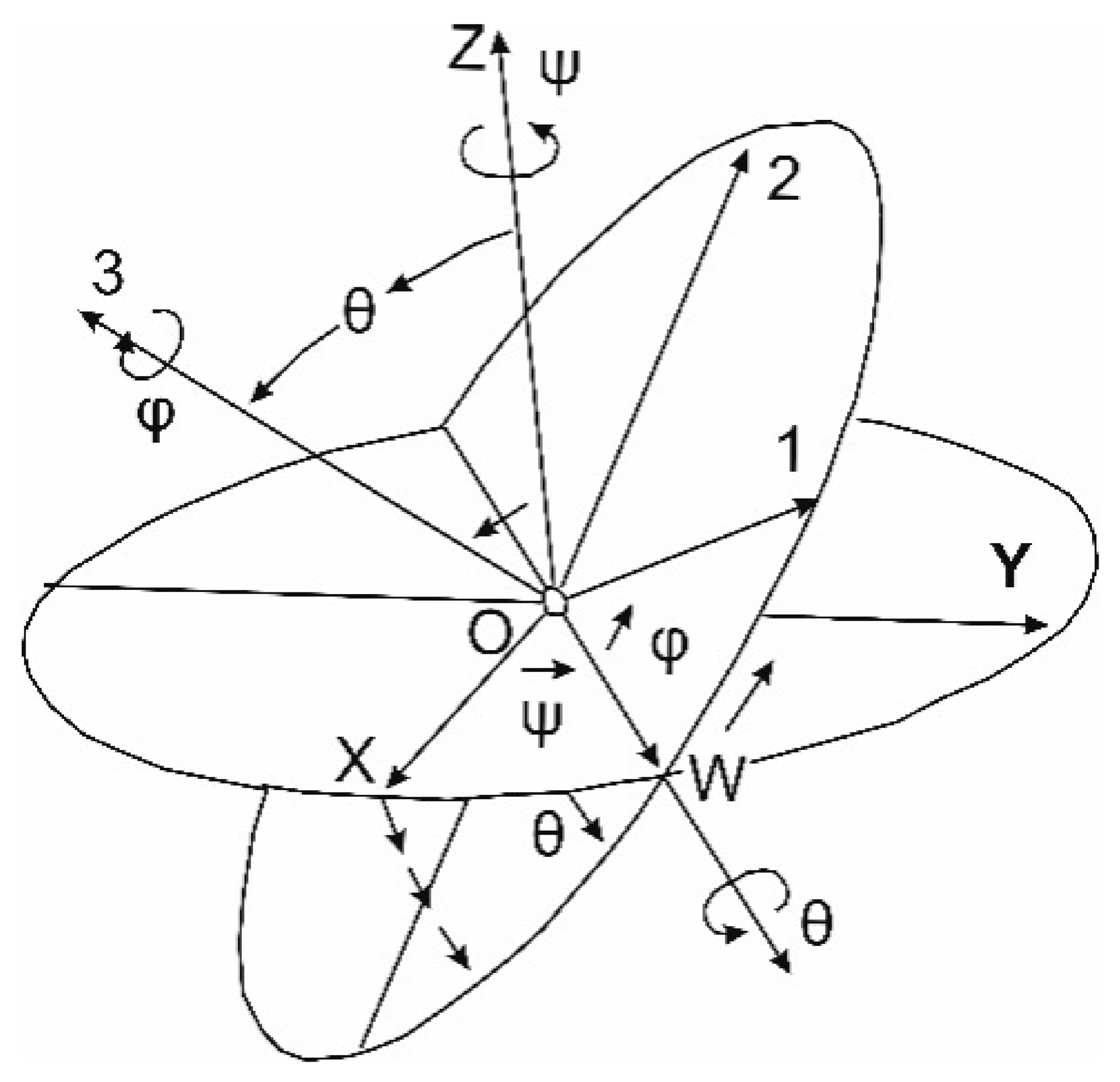
- ψ—precession angle, between the axis and the node line (rotation around the Z axis),
- θ—nutation angle, between the and axes (rotation around the node line),
- φ—angle of pure rotation (intrinsic rotation), between the line of nodes and the axis (rotation around axis 3).
- rotation order: ω → φ → κ,
- ω—the rotation around the X axis (clockwise), the roll angle,
- φ—the rotation around the Y axis (anticlockwise), the pitch angle,
- κ—the rotation around the Z axis (clockwise), the yaw angle.
- rotation order: ψ → θ → φ,
- ψ—yaw angle (anticlockwise), rotation around the Z axis,
- θ—pitch angle (clockwise), rotation around the Y axis (after rotation around the Z axis),
- φ—roll angle (anticlockwise), rotation around the X axis (after rotation around the Z and Y axes).
- I—identity matrix.
- ψ, θ, φ—infinitesimal values of angles expressed in radians, the angles are the same as in Equation (5).
- —rotation angle around the Z axis,
- —rotation angle around the Y axis,
- —rotation angle around the X axis,
- —scale factor, where ds corresponds to linear system distortion,
- —translation vector.
- —coordinates in the average Earth coordinate system,
- —coordinates in a geodetic (local) coordinate system,
- —(infinitesimal) rotation angles expressed in radians,
- —scale correction,
- —vector of translation in the terrestrial system,
- —translation vector in the geodetic (local) system,
- —the coordinates of the origin of the geodetic (local) coordinate system after rotation and shift to the mean terrestrial system.
- —coordinates in the geodetic (local) system after moving to the centroid, the center of gravity of this system,
- indexes 1 and 2 next to the translation and coordinate vectors mean, respectively: 1—geodetic (local) system, 2—Earth system.
- X—vector of unknown parameters,
- A—matrix of coefficients with unknowns (partial derivatives)—Jacobian transformation,
- L—vector of constants,
- P—vector of weighting factors (statistical weights).
2. Materials and Methods
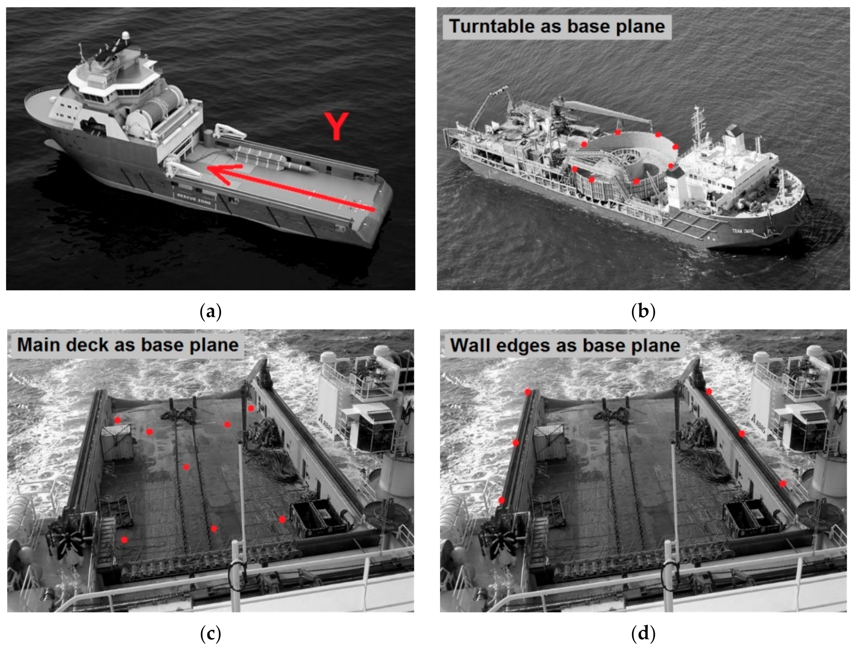
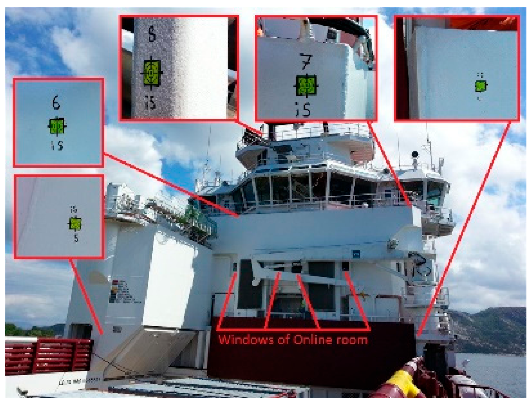
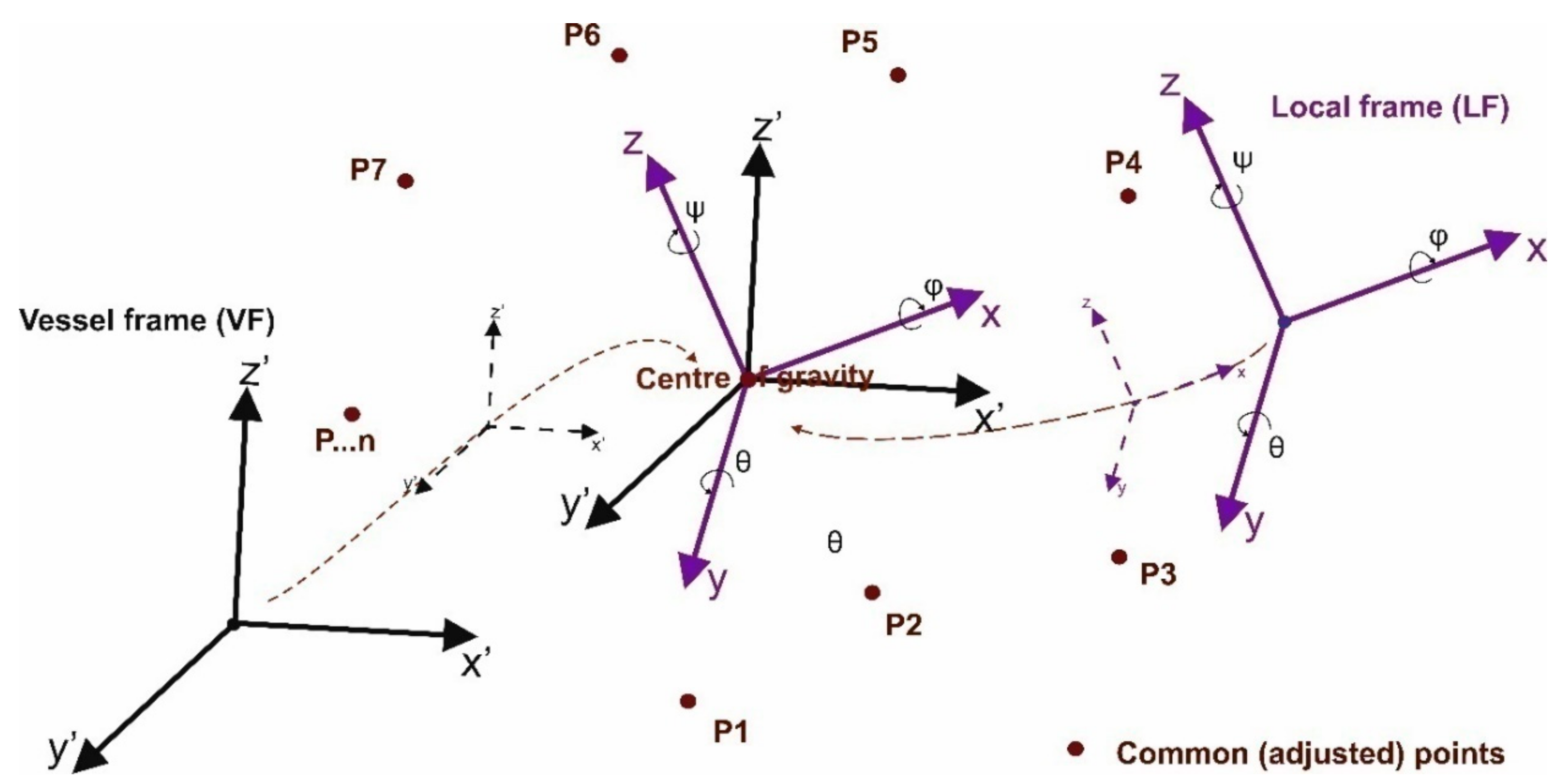
2.1. Vessel Offsets Measurements
- Sensors of interest (the purpose of the survey),
- Sensors for connecting the survey to a pre-established coordinate frame of vessel system (USBL, DP),
- Ship elements for connecting the survey to General Arrangement (GA) drawing of a vessel,
- Prepared pitch, roll and heading calibration points,
- Ship body for alignment and positioning of the new local coordinate frame:
- Z-axis direction (base plane),
- Y-axis direction,
- Origin X-position (center line of vessel),
- Origin Y-position,
- Origin Z-position.
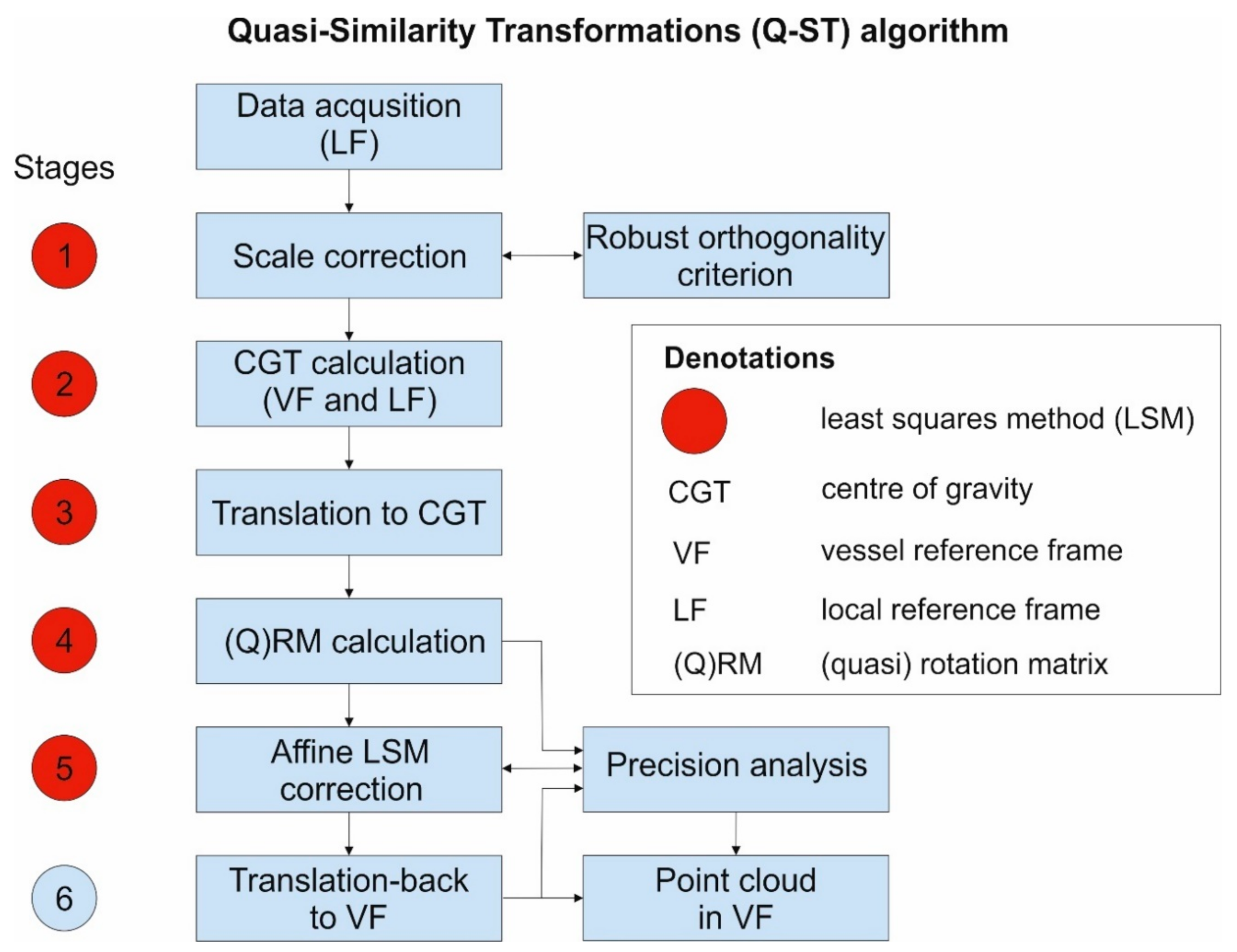
2.2. Quasi-Similarity Transformations (Q-ST) Algorithm
- —coordinates in the target system—stationary (vessel reference frame—VF),
- —rotation matrix,
- —scale factor,
- —coordinates in the transformed system (local reference frame—LF),
- —coordinates of the center of gravity in the transformed system (centroid of local reference frame),
- —coordinates of the center of gravity in the target system—stationary (centroid of vessel reference frame).
- —vector length in the ship’s coordinate system (VF),
- —the length of the vector in the local coordinate system associated with the instrument (LF).
- —a vector consisting of the length of the homologous vectors in the local LF system,
- —a vector consisting of the lengths of the homologous vectors in the VF ship system,
- —lengths of homologous vectors in the LF and VF coordinate systems,
- —the number of homolog vector pairs known in LF and VR.
- —length of the homologous vector in each of the LF and VF systems built using two points: the center of gravity and the considered fit point,
- —coordinates of the center of gravity (center of mass) in LF and VF respectively,
- —the coordinates of the fitting point, i ∈ (1,2, ..., n),
- —number of homologous points, adjustments (common points) in LF and RF systems.
- —centroid coordinates of points in the LF and VF systems related to the center of gravity,
- —centroid coordinates of points in the VF system.
- —a rotation matrix defined by Equation (9),
- , —designations as in Equation (33).
- —number of matching points,
- —number of observations (adjustment points) necessary to carry out the transformation (in the considered transformation model,
2.3. Software
3. Results
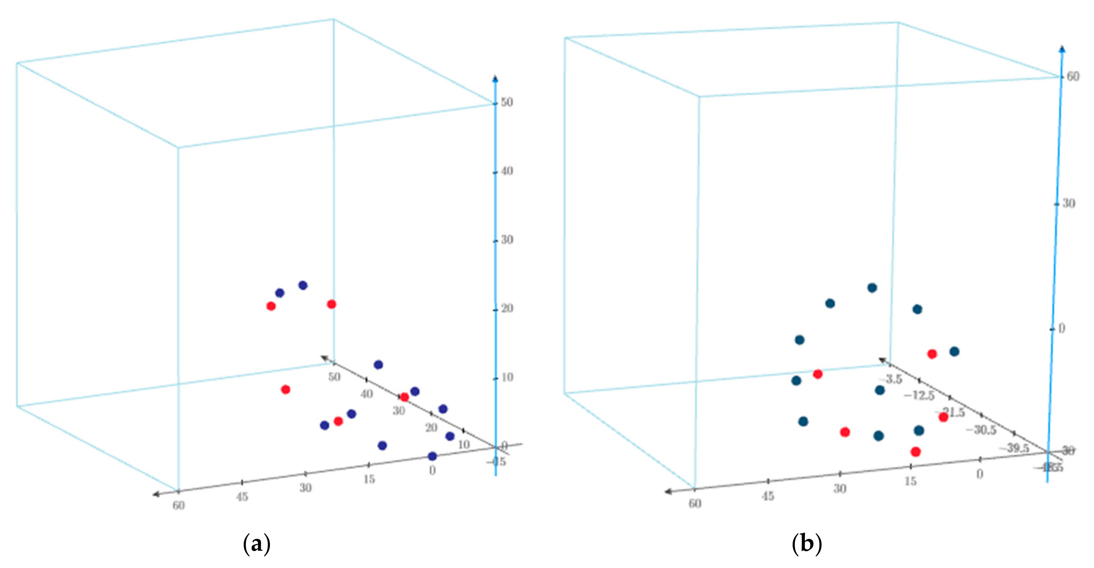
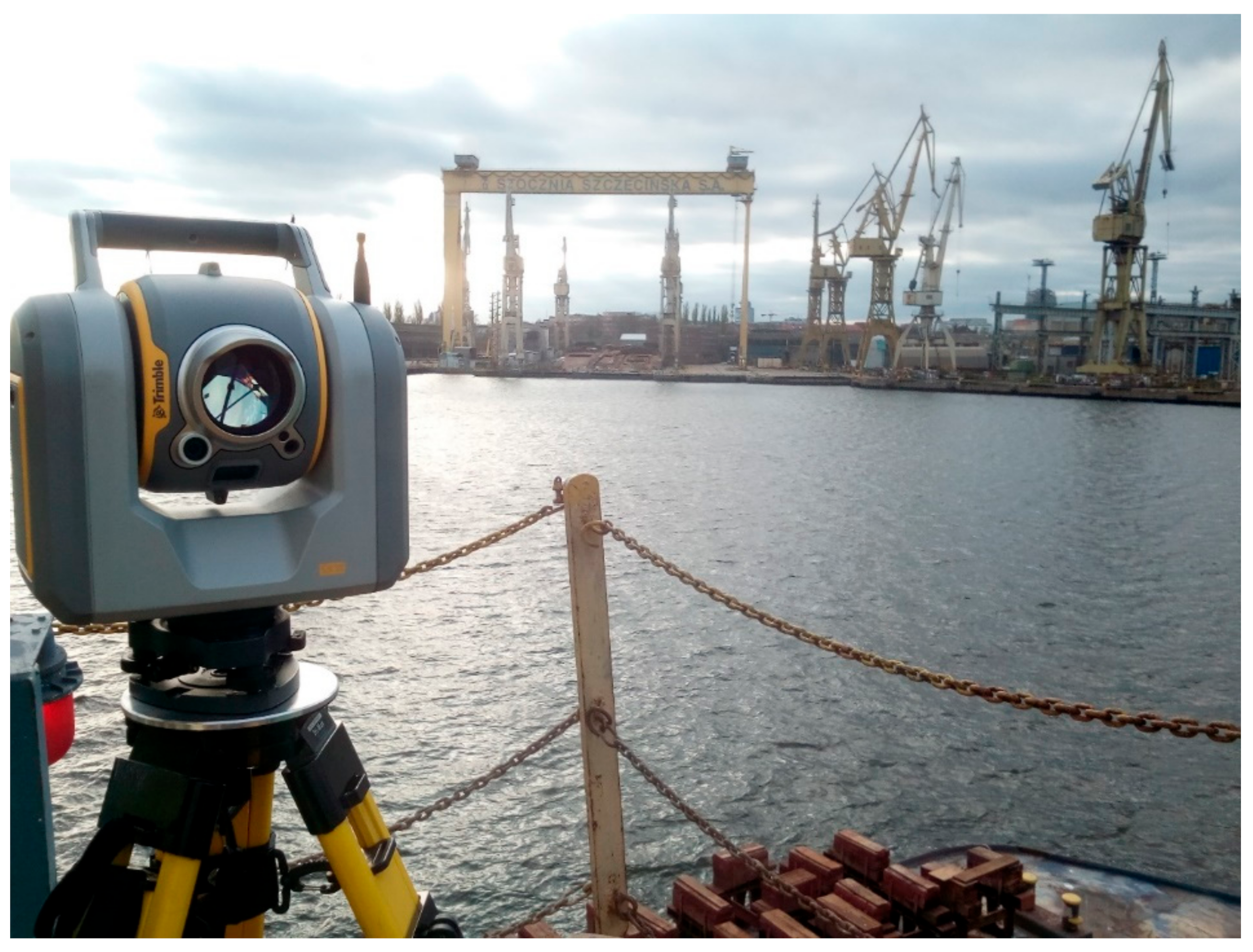
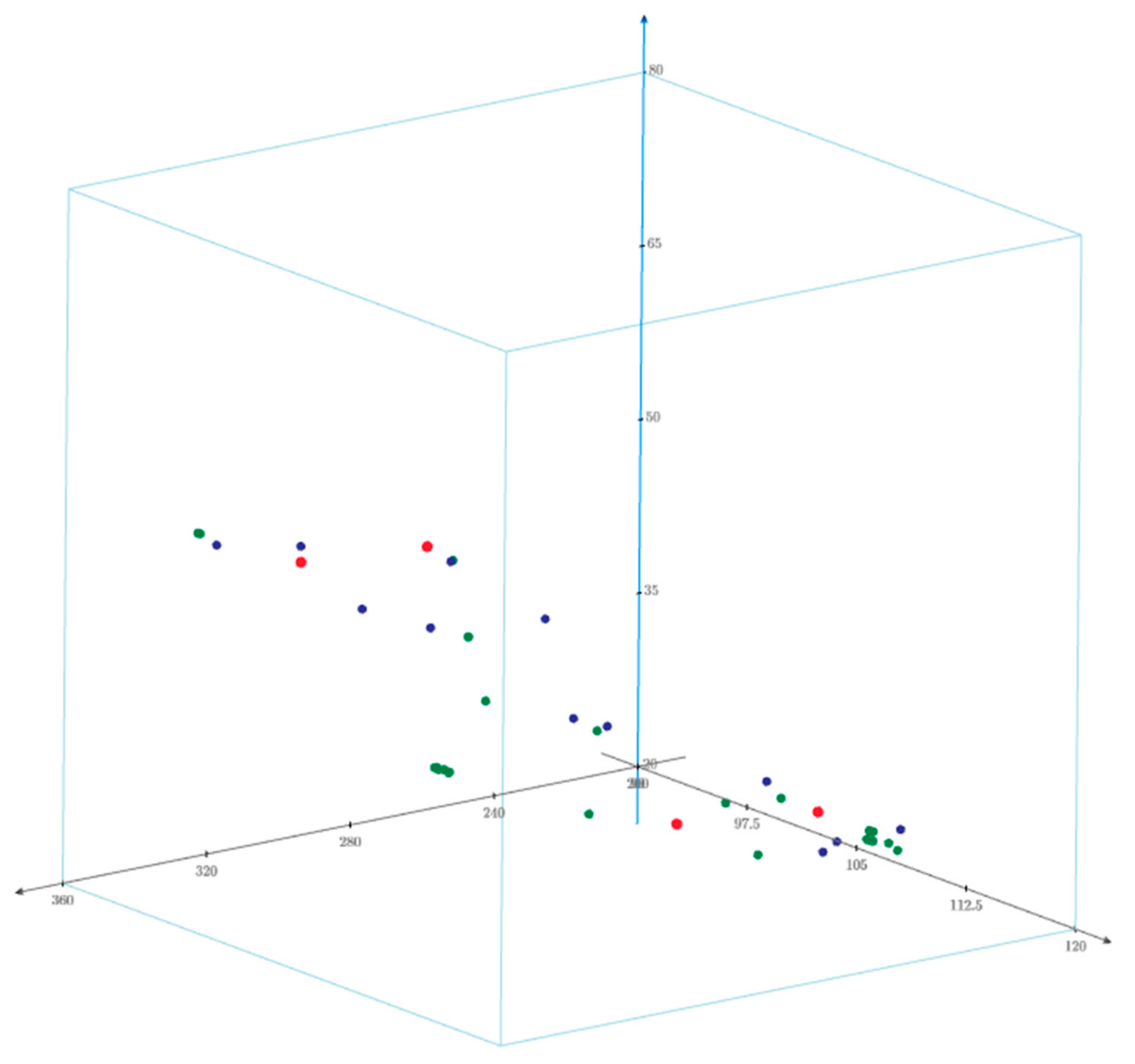
3.1. Description of the Experiment
3.2. Experiment
4. Discussion and Conclusions
Author Contributions
Funding
Acknowledgments
Conflicts of Interest
References
- Deakin, R.E. 3-D coordinate transformations. Surv. L. Inf. Syst. 1998, 58, 223–234. [Google Scholar]
- Grewal, M.S.; Weill, L.R.; Andrews, I.A.P. Global Positioning Systems, Inertial Navigation, and Integration, 2nd ed.; John Wiley & Sons: Hoboken, NJ, USA, 2006. [Google Scholar]
- Soler, T. A compendium of transformation formulas useful in GPS work. J. Geod. 1998, 72, 482–490. [Google Scholar] [CrossRef]
- Luhmann, T.; Robson, S.; Kyle, S.; Boehm, I.J. Close-Range Photogrammetry and 3D Imaging, 2nd ed.; Walter de Gruyter: Berlin/Boston, Germany, 2014. [Google Scholar]
- Colomina, I.; Molina, P. Unmanned aerial systems for photogrammetry and remote sensing: A review. ISPRS J. Photogramm. Remote Sens. 2014, 92, 79–97. [Google Scholar] [CrossRef]
- Brazeal, R. Three dimensional coordinate transformations for registering terrestrial laser scanning datasets based on tie points. Point Cloud Anal. 2013, SUR 6905. [Google Scholar] [CrossRef]
- Huang, J.; You, S. Point cloud matching based on 3D self-similarity. In Proceedings of the 2012 IEEE Computer Society Conference on Computer Vision and Pattern Recognition Workshops, Providence, RI, USA, 16–21 June 2012. [Google Scholar]
- Brazetti, L.; Scaioni, M. Automatic orientation of image sequences for 3D object reconstruction: first results of a method integrating photogrammetric and computer vision algorithms. In Proceedings of the 3D-ARCH 2009: 3D Virtual Reconstruction and Visualization Workshop, Trento, Italy, 25–28 February 2009. [Google Scholar]
- Schofield, W.; Breach, M. Engineering Surveying, 6th ed.; CRC Press: Boca Raton, FL, USA, 2007. [Google Scholar]
- Kilford, W.K. Surveying for Engineers. Surv. Rev. 1979, 25, 94–96. [Google Scholar] [CrossRef]
- Tu, Y. Machine learning. In EEG Signal Processing and Feature Extraction; Springer: Berlin/Heidelberg, Germany, 2019; pp. 301–323. [Google Scholar]
- Zuur, A.F.; Ieno, E.N.; Smith, G.M. Principal coordinate analysis and non-metric multidimensional scaling. In Analysing Ecological Data; Springer: Berlin/Heidelberg, Germany, 2007; pp. 259–264. [Google Scholar]
- Graf, M. Coordinate transformations in object recognition. Psychol. Bull. 2006, 132, 920–945. [Google Scholar] [CrossRef] [PubMed]
- Baetslé, P.-L. Conformal transformations in three dimensions. Photogramm Eng. Remote Sens. 1966, 32, 816–824. [Google Scholar]
- Stark, M. Geometra Analityczna z Wstępem do Geometrii Wielowymiarowej, 6th ed.; Państwowe Wydawnictwo Naukowe: Warszawa, Poland, 1974. (In Polish) [Google Scholar]
- Kutoglu, H.S.; Mekik, C.; Akcin, H. A comparison of two well known models for 7-parameter transformation. Aust. Surv. 2002, 47, 24–30. [Google Scholar] [CrossRef]
- Stępień, G. Transformacje Symetryczne w Nachylonych Układach Odniesienia z Wykorzystaniem Metod Analizy Funkcjonalnej; Wydawnictwo Naukowe Akademii Morskiej w Szczecinie: Szczecin, Poland, 2018. (In Polish) [Google Scholar]
- Schut, G.H. Similarity Transformation and least Squares. Photogramm. Eng. 1973, 39, 621–627. [Google Scholar]
- Diebel, J. Representing attitude: Euler angles, unit quaternions, and rotation vectors. Matrix 2006, 58, 1–35. [Google Scholar]
- Titterton, D.; Weston, J. Strapdown Inertial Navigation Technology, 2nd ed.; IET: London, UK, 2004. [Google Scholar]
- Baranowski, L. Equations of Motion of a Spin-Stabilized Projectile for Flight Stability Testing. J. Theor. Appl. Mech. 2013, 51, 235–246. [Google Scholar]
- Allgeuer, P.; Behnke, S. Fused Angles and the Deficiencies of Euler Angles. In Proceedings of the 2018 IEEE/RSJ International Conference on Intelligent Robots and Systems (IROS), Madrid, Spain, 1–5 October 2018. [Google Scholar]
- Henderson, D. Euler Angles, Quaternions, and Transformation Matrices; Technical Memorandum for NASA, Lyndon B. Johnson Space Center: Houston, TX, USA, 1997. [Google Scholar]
- Kielich, S. Molekularna Optyka Nieliniowa; Państwowe Wydawnictwo Naukowe: Warszawa-Poznań, Poland, 1977. (In Polish) [Google Scholar]
- Liu, H.; Fang, Y. Direct 3D coordinate transformation based on the affine invariance of barycentric coordinates. J. Spat. Sci. 2019. [Google Scholar] [CrossRef]
- Andrei, C. 3D Affine Coordinate Transformations. Master’s Thesis, School of Architecture and the Built Environment Royal Institute of Technology (KTH), Stockholm, Sweden, March 2006. [Google Scholar]
- Späth, H. A Numerical Method for Determining the Spatial HELMERT Transformation in the Case of Different Scale Factors. Fachbeiträge 2004, 6, 255–257. [Google Scholar]
- Wolf, H. Geometric connection and re-orientation of three-dimensional triangulation nets. J. Geod. 1963, 68, 165–169. [Google Scholar] [CrossRef]
- Deakin, R. A note on the Bursa-Wolf and Molodensky-Badekas transformations; Bulletin for the School of Mathematican and Geospatial Sciences; RMIT University: Merlbourne, Australia, 2006. [Google Scholar]
- Badekas, J. Establishment of an Ideal World Geodetic System. Ph.D. Thesis, The Ohio State University, Columbus, OH, USA, 1969. [Google Scholar]
- Dare, O.P.; Okiemute, E.S.; Eteje, S.O. Impact of different centroid means on the accuracy of orthometric height modelling by geometric geoid method. Int. J. Sci. Rep. 2020, 6, 124–130. [Google Scholar] [CrossRef]
- Jue, L. Research on close-range photogrammetry with big rotation angle. Int. Arch. Photogramm. Remote Sens. Spat. Inf. Sci. 2008, 1, 11–14. [Google Scholar]
- Acar, M.; Özlüdemir, M.T.; Akyilmaz, O.; Çelik, R.N.; Ayan, T. Deformation analysis with Total Least Squares. Nat. Hazards Earth Syst. Sci. 2006, 6, 663–669. [Google Scholar] [CrossRef]
- Qin, Y.; Fang, X.; Zeng, W.; Wang, B. General Total Least Squares Theory for Geodetic Coordinate Transformations. Appl. Sci. 2020, 10, 2598. [Google Scholar] [CrossRef]
- Brandt, S. Data Analysis: Statistical and Computational Methods for Scientists and Engineers, 4th ed.; North-Holland Publishing Company: Amsterdam, The Netherlands, 2014. [Google Scholar]
- Taylor, J.R.; Thompson, W. An Introduction to Error Analysis: The Study of Uncertainties in Physical Measurements. Phys. Today 1998, 51, 57–58. [Google Scholar] [CrossRef]
- Czarnecki, K. Geodezja Współczesna w Zarysie; Wydawnictwo Wiedza i Życie: Warszawa, Poland, 1995. (In Polish) [Google Scholar]
- Wrona, W. Matematyka; Państwowe Wydawnictwo Naukowe: Warszawa, Poland, 1964. (In Polish) [Google Scholar]


| Value | |||||||
| 38.57893 | 33.30716 | 227.35478 | 1.000000 |
| Point | Vessel Frame—VF | Local Frame—LF | ||||
|---|---|---|---|---|---|---|
| X (m) | Y (m) | Z (m) | X (m) | Y (m) | Z (m) | |
| 1. | 0.000 | 0.000 | 0.000 | −14.006 | −2.300 | −3.815 |
| 2. | 5.000 | −8.000 | 1.000 | −12.468 | 6.188 | −7.763 |
| 3. | 15.000 | −14.000 | 2.000 | −14.990 | 14.829 | −15.244 |
| 4. | 25.000 | −15.000 | 2.000 | −20.037 | 19.041 | −22.846 |
| 5. | 35.000 | −14.000 | 3.500 | −27.137 | 22.472 | −29.255 |
| 6. | 15.000 | 14.000 | 2.000 | −32.203 | −7.053 | −12.257 |
| 7. | 5.000 | 8.000 | 1.000 | −22.304 | −6.315 | −6.055 |
| 8. | 25.000 | 0.000 | 0.000 | −28.160 | 6.276 | −22.553 |
| 9. | 40.000 | 0.000 | 15.000 | −44.890 | 19.239 | −23.995 |
| 10. | 38.000 | 7.000 | 15.000 | −48.060 | 13.083 | −21.749 |
| 11. | 16.000 | 10.000 | 2.000 | −30.310 | −3.584 | −13.433 |
| 12. | 23.000 | −11.000 | 2.000 | −21.364 | 15.229 | −20.920 |
| 13. | 39.000 | −6.000 | 12.000 | −38.988 | 22.022 | −25.846 |
| 14. | 42.000 | 6.000 | 12.000 | −48.063 | 13.673 | −26.814 |
| 15. | 31.000 | 11.000 | 3.000 | −39.967 | 1.302 | −23.916 |
| Transformation | No. of Common (Adjusted) Points | Mean Errors on Common (Adjusted) Points (mm) | Mean Errors on Check Points (mm) | ||||||
|---|---|---|---|---|---|---|---|---|---|
| Q-ST | 5 | 0.00 | 0.00 | 0.00 | 0.00 0.00 | 0.00 | 0.00 | 0.00 | 0.00 |
| SC4W | 0.33 | 0.10 | 0.18 | 0.38 | 0.42 | 0.49 | 0.70 | 0.96 | |
| Geonet DC | 0.33 | 0.10 | 0.18 | 0.39 | 0.42 | 0.49 | 0.71 | 0.96 | |
| Q-ST | 4 | 0.00 | 0.00 | 0.00 | 0.00 0.00 | 0.00 | 0.00 | 0.00 | 0.00 |
| SC4W | 0.33 | 0.14 | 0.20 | 0.41 | 0.44 | 0.52 | 0.72 | 1.00 | |
| Geonet DC | 0.33 | 0.09 | 0.28 | 0.44 | 0.49 | 0.49 | 0.96 | 1.18 | |
| Value | |||||||
| 27.35478 | 1.30716 | 1.57894 | 1.000000 |
| Point | dX (m) | dY (m) | dZ (m) |
|---|---|---|---|
| 1. | −0.0009 | −0.0014 | −0.0008 |
| 2. | −0.0014 | −0.0010 | −0.0013 |
| 3. | −0.0009 | 0.0011 | −0.0003 |
| 4. | −0.0019 | −0.0005 | 0.0020 |
| 5. | −0.0034 | 0.0002 | 0.0004 |
| 6. | 0.0020 | −0.0058 | 0.0009 |
| 7. | 0.0017 | −0.0043 | −0.0010 |
| 8. | 0.0018 | 0.0004 | −0.0014 |
| 9. | 0.0013 | −0.0012 | 0.0061 |
| 10. | −0.0021 | −0.0024 | −0.0006 |
| 11. | 0.0001 | 0.0002 | −0.0026 |
| 12. | −0.0015 | 0.0015 | 0.0015 |
| 13. | 0.0014 | 0.0006 | −0.0008 |
| 14. | −0.0004 | 0.0000 | −0.0024 |
| 15. | −0.0013 | −0.0015 | −0.0021 |
| Mean error— Calculated () | 0.0017 | 0.0022 | 0.0021 |
| Point | Vessel Frame—VF | Local Frame—LF | ||||
|---|---|---|---|---|---|---|
| X (m) | X (m) | X (m) | X (m) | Y (m) | Z (m) | |
| 1. | 28.8670 | 28.8670 | 28.8680 | 51.967 | 7.250 | 31.873 |
| 2. | 28.8670 | −28.8670 | 28.8680 | 25.445 | −44.025 | 32.681 |
| 3. | −28.8670 | 28.8670 | 28.8680 | 0.702 | 33.739 | 29.974 |
| 4. | −28.8670 | −28.8670 | 28.8680 | −25.821 | −17.538 | 30.784 |
| 5. | 28.8670 | 28.8670 | −28.8680 | 53.281 | 5.661 | −25.825 |
| 6. | 0.0000 | 35.3550 | 35.3550 | 29.170 | 26.430 | 37.317 |
| 7. | 0.0000 | −35.3550 | −35.3550 | −1.700 | −38.316 | −32.360 |
| 8. | 35.3550 | 35.3550 | 0.0000 | 61.370 | 9.242 | 3.146 |
| 9. | −35.3550 | −35.3550 | 0.0000 | −33.900 | −21.120 | 1.816 |
| 10. | 0.0000 | −50.0000 | 0.0000 | −9.238 | −50.347 | 3.178 |
| 11. | 50.0000 | 0.0000 | 0.0000 | 58.130 | −28.876 | 4.122 |
| 12. | −50.0000 | 0.0000 | 0.0000 | −30.666 | 17.002 | 0.834 |
| 13. | 0.0000 | 0.0000 | 50.0000 | 12.594 | −4.560 | 52.446 |
| 14. | 0.0000 | 50.0000 | 0.0000 | 36.702 | 38.468 | 1.776 |
| 15. | 0.0000 | 0.0000 | −50.0000 | 14.872 | −7.317 | −47.492 |
| Transformation | No. of Common (Adjusted) Points | Mean Errors on Common (Adjusted) Points (mm) | Mean Errors on Check Points (mm) | ||||||
|---|---|---|---|---|---|---|---|---|---|
| Q-ST | 5 | 0.57 | 0.03 | 0.50 | 0.76 | 2.27 | 3.03 | 2.89 | 4.77 |
| SC4W | 1.06 | 0.94 | 1.35 | 1.95 | 2.70 | 2.34 | 2.80 | 4.54 | |
| Geonet DC | 1.16 | 0.47 | 1.03 | 1.62 | 2.81 | 2.54 | 2.40 | 4.48 | |
| Q-ST | 4 | 0.00 | 0.00 | 0.00 | 0.00 0.00 | 2.84 | 2.75 | 2.07 | 4.46 |
| SC4W | 1.25 | 0.38 | 0.97 | 1.62 | 2.84 | 2.49 | 2.07 | 4.31 | |
| Geonet DC | 1.25 | 0.38 | 0.97 | 1.63 | 2.84 | 2.49 | 2.07 | 4.31 | |
| Point Number ST1 | Common Points | ||
|---|---|---|---|
| ST2 | ST3 | ST4 | |
| 1 | + | + | |
| 2 | + | + | |
| 3 | + | ||
| 5 | + | ||
| 6 | + | ||
| 7 | + | ||
| M1 | + | + | |
| M2 | + | + | + |
| M3 | + | ||
| M4 | + | ||
| M11 | + | ||
| Suma | 6 | 5 | 5 |
| Station ST1 | X (m) (North) | Y (m) (East) | Z (m) (Up) |
|---|---|---|---|
| Point Number | |||
| 1 | 234.752 | 116.514 | 29.169 |
| 2 | 235.198 | 107.448 | 29.096 |
| 3 | 260.012 | 100.302 | 32.768 |
| 5 | 333.558 | 93.845 | 49.364 |
| 6 | 337.931 | 104.895 | 49.292 |
| 7 | 334.844 | 108.814 | 49.302 |
| M1 | 259.083 | 117.185 | 29.061 |
| M2 | 299.949 | 101.61 | 49.456 |
| M3 | 319.777 | 96.212 | 49.505 |
| M4 | 307.113 | 109.849 | 48.809 |
| M11 | 257.723 | 102.046 | 32.763 |
| Station ST2 | X (m) (North) | Y (m) (East) | Z (m) (Up) | Common Point (Yes—Y/No—N) |
|---|---|---|---|---|
| Point Number | ||||
| ST2 | 300.000 | 100.000 | 50.000 | N |
| M2 | 264.588 | 99.054 | 48.506 | Y |
| 5 | 298.653 | 93.677 | 48.469 | Y |
| 6 | 302.242 | 105.017 | 48.403 | Y |
| 7 | 298.884 | 108.703 | 48.410 | Y |
| M4 | 271.151 | 107.780 | 47.873 | Y |
| FUGRO_STBD_C | 273.766 | 102.844 | 56.104 | N |
| FUGRO_PORT_C | 273.770 | 100.120 | 56.141 | N |
| FUGRO_PORT_1 | 273.822 | 100.169 | 56.188 | N |
| FUGRO_PORT_2 | 273.844 | 100.131 | 56.189 | N |
| FUGRO_PORT_3 | 273.837 | 100.072 | 56.196 | N |
| FUGRO_PORT_4 | 273.813 | 100.049 | 56.187 | N |
| FUGRO_STB_1 | 273.810 | 102.910 | 56.147 | N |
| FUGRO_STB_2 | 273.832 | 102.874 | 56.143 | N |
| FUGRO_STB_3 | 273.831 | 102.834 | 56.141 | N |
| FUGRO_STB_4 | 273.810 | 102.797 | 56.144 | N |
| GPS_PORT_1 | 296.980 | 91.978 | 48.604 | N |
| GPS_PORT_2 | 297.054 | 91.978 | 48.602 | N |
| GPS_PORT_3 | 297.119 | 91.914 | 48.599 | N |
| GPS_PORT_4 | 296.945 | 91.956 | 48.604 | N |
| GPS_PORT_5 | 297.022 | 91.984 | 48.603 | N |
| GPS_PORT_6 | 297.125 | 91.882 | 48.599 | N |
| GPS_STBD_1 | 297.020 | 110.743 | 48.519 | N |
| GPS_STBD_2 | 296.966 | 110.711 | 48.519 | N |
| GPS_STBD_3 | 296.888 | 110.722 | 48.518 | N |
| GPS_STBD_4 | 296.925 | 110.709 | 48.518 | N |
| GPS_STBD_5 | 296.995 | 110.722 | 48.519 | N |
| GPS_STBD_6 | 297.032 | 110.762 | 48.518 | N |
| M3 | 284.740 | 95.070 | 48.588 | Y |
| Station ST3 | X (m) (North) | Y (m) (East) | Z (m) (Up) | Common Point (Yes—Y/No—N) |
|---|---|---|---|---|
| Point Number | ||||
| ST3 | 300.000 | 100.000 | 50.000 | N |
| M2 | 325.598 | 92.445 | 69.835 | Y |
| M1 | 283.660 | 104.852 | 49.435 | Y |
| 1 | 259.446 | 102.306 | 49.537 | Y |
| 2 | 260.589 | 93.302 | 49.451 | Y |
| 3 | 285.881 | 88.085 | 53.128 | Y |
| USBL_1 | 307.939 | 86.696 | 48.413 | N |
| USBL_2 | 308.280 | 86.765 | 48.408 | N |
| USBL_3 | 307.707 | 86.259 | 48.421 | N |
| USBL_4 | 307.968 | 85.836 | 48.419 | N |
| USBL_5 | 308.458 | 85.837 | 48.411 | N |
| USBL_6 | 308.697 | 86.172 | 48.404 | N |
| Station ST4 | X (m) (North) | Y (m) (East) | Z (m) (Up) | Common Point (Yes—Y/No—N) |
|---|---|---|---|---|
| Point Number | ||||
| ST4 | 300.000 | 100.000 | 50.000 | N |
| M2 | 356.008 | 90.648 | 69.726 | Y |
| M1 | 314.558 | 104.564 | 49.317 | Y |
| M11 | 313.816 | 89.377 | 53.002 | Y |
| 1 | 290.266 | 102.901 | 49.412 | Y |
| 2 | 291.082 | 93.860 | 49.329 | Y |
| PRISM_SF | 328.338 | 104.061 | 49.454 | N |
| PRISM_SA | 300.156 | 104.953 | 49.644 | N |
| PRISM_PA | 299.529 | 84.558 | 49.710 | N |
| Transformation | No. of Common (Adjusted) Points | Mean Errors on Common (Adjusted) Points (mm) | Average Errors on Common (Adjusted) Points (mm) | ||||||
|---|---|---|---|---|---|---|---|---|---|
| Q-ST | 6 (ST2 to ST1) | 1.86 | 2.34 | 0.75 | 3.09 | 1.44 | 1.82 | 0.55 | 2.39 |
| SC4W | 3.19 | 3.00 | 0.89 | 4.47 | 2.50 | 1.83 | 0.67 | 3.17 | |
| Geonet DC | 3.24 | 2.88 | 0.92 | 4.43 | 2.54 | 1.92 | 0.77 | 3.28 | |
| Q-ST | 5 (ST3 to ST1) | 0.55 | 0.20 | 1.48 | 1.59 | 0.43 | 0.16 | 1.16 | 1.25 |
| SC4W | 3.81 | 1.32 | 2.29 | 4.64 | 3.20 | 1.00 | 1.80 | 4.54 | |
| Geonet DC | 3.61 | 1.29 | 2.13 | 4.39 | 2.99 | 1.00 | 1.78 | 3.62 | |
| Q-ST | 5 (ST4 to ST1) | 1.31 | 0.12 | 0.32 | 1.350.00 | 1.03 | 0.10 | 0.26 | 1.07 |
| SC4W | 4.30 | 0.71 | 2.06 | 4.82 | 3.60 | 0.40 | 1.80 | 4.04 | |
| Geonet DC | 4.56 | 0.80 | 1.93 | 5.02 | 3.80 | 0.52 | 1.68 | 4.19 | |
Publisher’s Note: MDPI stays neutral with regard to jurisdictional claims in published maps and institutional affiliations. |
© 2020 by the authors. Licensee MDPI, Basel, Switzerland. This article is an open access article distributed under the terms and conditions of the Creative Commons Attribution (CC BY) license (http://creativecommons.org/licenses/by/4.0/).
Share and Cite
Stępień, G.; Tomczak, A.; Loosaar, M.; Ziębka, T. Dimensioning Method of Floating Offshore Objects by Means of Quasi-Similarity Transformation with Reduced Tolerance Errors. Sensors 2020, 20, 6497. https://doi.org/10.3390/s20226497
Stępień G, Tomczak A, Loosaar M, Ziębka T. Dimensioning Method of Floating Offshore Objects by Means of Quasi-Similarity Transformation with Reduced Tolerance Errors. Sensors. 2020; 20(22):6497. https://doi.org/10.3390/s20226497
Chicago/Turabian StyleStępień, Grzegorz, Arkadiusz Tomczak, Martin Loosaar, and Tomasz Ziębka. 2020. "Dimensioning Method of Floating Offshore Objects by Means of Quasi-Similarity Transformation with Reduced Tolerance Errors" Sensors 20, no. 22: 6497. https://doi.org/10.3390/s20226497
APA StyleStępień, G., Tomczak, A., Loosaar, M., & Ziębka, T. (2020). Dimensioning Method of Floating Offshore Objects by Means of Quasi-Similarity Transformation with Reduced Tolerance Errors. Sensors, 20(22), 6497. https://doi.org/10.3390/s20226497