Blind Estimation Methods for BPSK Signal Based on Duffing Oscillator

Abstract

To realize the blind estimation of binary phase shift keying (BPSK) signal, this paper describe a new relational expression among the state of Duffing oscillator excited by BPSK signal, the pseudo-random code of BPSK signal, and the difference frequency between the to-be-detect signal and internal drive force signal of Duffing oscillator. Two output characteristics of Duffing oscillators excited by BPSK signals named implied periodicity and pilot frequency array synchronization are presented according to the different chaotic states of Duffing oscillator. Then two blind estimation methods for the carrier frequency and pseudo-random sequence of the BPSK signal are proposed based on these two characteristics, respectively. These methods are shown to have a significant effect on the parameter estimation of BPSK signals with no prior knowledge, even at very low signal-to-noise ratios (SNRs).

1. Introduction

In modern radar electronic warfare, reconnaissance and anti-reconnaissance efforts, as well as the evaluations of the reconnaissance effect, are of great importance. Obtaining useful information from enemy radar signals can provide guidance for radar jamming and fire destruction and enable effective countermeasures to be taken against enemy interference [1,2]. In the field of radar and communication, binary phase shift keying (BPSK) signals are commonly used because of their high frequency band utilization, strong anti-noise interference ability, wide signal bandwidth, and resistance to detection [3,4,5,6]. In actual battlefield situations, there is often a complex electromagnetic environment and electronic countermeasures under non-cooperative conditions, and so useful signals are often drowned in strong noise, complicating the tasks of efficient intercepted efficiently and accurate estimated. For these reasons, blind detection of the weak BPSK signals at low signal-to-noise ratios (SNRs) is an important subject.

Part of the literatures focuses on the estimation of carrier frequency. Methods based on the cyclic spectrum density [7], second-order cyclic statistics [8], and stochastic resonance (SR) [9] have been developed to estimate carrier frequency and symbol rate of BPSK signal, but these methods cannot calculate the pseudo-random code, and their estimation accuracy is poor in low SNR environments (the SNR should be greater than −6 dB, −2 dB, and 0 dB, respectively). The other part of the research estimates the pseudo-random sequence. Wang et al. [10] estimate the period and staring bit of pseudo-random sequence through the method of reprocessing the power spectrum density, segmentation processing, and an average cross-correlation calculation, which can be realized even the SNR = −15 dB, but the carrier frequency needs to be known in advance. Synchronous demodulation method can identify pseudo-random codes effectively and provide easier parameter estimation algorithm [11], but this approach needs to exact the carrier frequency before estimating the pseudo-random code. Some estimators based on cyclic spectral density function were proposed in [12,13], which has less computationally intensive, but the chip time width and carrier frequency should be known. In the above methods, only carrier frequency estimation is not enough, but the estimation of pseudo-random code requires prior knowledge or additional calculation, which requires time accumulation or multiple processing. Moreover, most of these methods have poor performance at low SNR and cannot be applied to the complex electromagnetic environment.

Because of the sensitivity to regular signals and immunity to noise under certain conditions, Duffing oscillators have often been used to detect weak signals [14,15,16,17]. The intermittent chaotic states in chaotic systems are known to enhance the practicability of weak signal detection in chaotic systems [18]. Recently, many methods for estimating the carrier frequency of BPSK signals using a Duffing oscillator have been developed [19,20], which can have great performance at very low SNR due to the Duffing oscillator. However, the pseudo-random sequence cannot be detected. The pseudo-random sequence estimation using the output characteristics of the Duffing oscillator excited by a known carrier frequency signal are studied in [21,22]. These methods are more easily to be calculated than the usual, but the carrier frequency of the BPSK signal at low SNR is not generally known under non-cooperative conditions. In short, these methods based on Duffing oscillator are limited in some way, but there have been few attempts to estimate both the carrier frequency and pseudo-random code of BPSK signals without prior knowledge using the Duffing oscillator.

In this paper, the relational expression among the state of Duffing oscillator, the phase code and the cosine function of the difference frequency in the intermittent chaotic state of the Duffing chaotic oscillator excited by BPSK signal is derived. Two parameter estimation methods for the joint estimation of carrier frequency and pseudo-random code based on this output characteristics are presented. These methods enable exact parameter estimations to be generated, even when no prior knowledge is available. Simulation and experiment results show that these methods have low computation complexity and high estimation precision, remain feasible in low SNR environments, and eliminate the high dependence of the traditional BPSK signal estimation method on the signal carrier frequency.

The remainder of paper is organized as follows. The next section analyzes the output characteristics of the BPSK signal in the Duffing oscillator system and deduces their relationship. In Section 3, the two blind parameter estimation methods are described. The simulation and experiment results in Section 4 demonstrate the feasibility of the proposed methods. Finally, the conclusions to this study are presented in Section 5.

2. Relationship among Functions in Duffing Oscillator System under Intermittent Chaotic State Excited by BPSK Signal

Traditional weak signal detection systems based on Duffing oscillator are excited by a standard sinusoidal signal, which can be expressed as

$$\{\begin{array}{l}\dot{x}=\omega y\\ \dot{y}=\omega (-ky+ax-b{x}^3+{\gamma }_{\mathrm{r}}\cos (\omega t)+{\gamma }_{\mathrm{s}}\cos ((\omega +\mathsf{\Delta }\omega )t+{\phi }_0)+n(t))\end{array}$$

(1)

where x is displacement, k is the damping coefficient, and −ax(t) + bx³(t) is the nonlinear restoring force. As shown in previous works, if we fix k = 0.5, a = b = 1, the Duffing oscillator system is more stable and represents better chaotic states [11,12,13,14]. γ_rcos(ωt) is a periodic internal driving force with an amplitude of γ_r ≈ γ_c, where γ_c is the critical threshold. γ_scos((ω+Δω)t + φ₀) is the to-be-detected signal. γ_s is the amplitude, φ₀ is the initial phase, and Δω is the frequency difference between the internal drive force signal and to-be-detected signal. n(t) is the stochastic disturbance, which is considered to be Gaussian white noise in this letter.

According to [18], the value of Δω can influence the equivalent driving force of the system, and then the chaotic states of Duffing oscillator can also change. If Δω = 0, after adding the signal to be measured, the system transforms from a chaotic state to a large-scale periodic state. If Δω ≠ 0, the system will be intermittently chaotic. When Δω ≤ 0.03ω, the intermittent chaotic state can be maintained regularly and stably. When Δω exceeds this limit, the intermittent chaotic state may be broken due to the insufficient maintenance time of the equivalent policy force. In weak signal detection, there is usually only a rough estimate for the frequency of the signal to be measured, which is often different from the drive signal frequency in the system. Thus, weak signal detection based on the intermittent chaotic state is universal and significant. Figure 1 illustrates the intermittent chaotic state of the Duffing oscillator excited by the standard sinusoidal signal. Here, ω = 100 MHz, Δω = 3 MHz, γ_r = 0.826, γ_s= 0.1, and φ₀ = 0.

BPSK signals can realize phase modulation using pseudo-random codes containing some sequence of 1 s and −1 s. They can be expressed as

$$s(t)={\gamma }_{\mathrm{s}}\cos ((\omega +\mathsf{\Delta }\omega )t+{\phi }_0+{\phi }_i)$$

(2)

where φ_i = (0, π) is the phase code of the BPSK signal. Replacing the sinusoidal signal to be detected in Equation (1) with the BPSK signal, the new state equation of the Duffing oscillator is

$$\{\begin{array}{l}\dot{x}=\omega y\\ \dot{y}=\omega (-0.5y+x-x^3+{\gamma }_{\mathrm{r}}\cos (\omega t)+{\gamma }_{\mathrm{s}}\cos ((\omega +\mathsf{\Delta }\omega )t+{\phi }_0+{\phi }_i)+n(t))\end{array}$$

(3)

Similar to the sinusoidal signal, BPSK signals can also cause the Duffing oscillator to transit intermittently between the chaotic state and large-scale periotic state if 0 < |Δω| ≤ 0.03ω. However, the duration of the different states is affected by both the difference frequency Δω and the phase code φ_i. Hence, the Duffing oscillator does not have a stable and regular intermittent chaotic period, unlike for the sinusoidal signal. The state in this condition is illustrated in Figure 2. Like the sinusoidal signal, we also fix ω = 100 MHz, Δω = 3 MHz, γ_r = 0.826, γ_s = 0.1, and φ₀ = 0.

To estimate the parameters of the BPSK signal, we need further analysis of the output characteristics of the Duffing oscillator. For Equation (3), the equivalent driving force of the system can be written as γ_ecos(ωt + θ), where

$${\gamma }_{\mathrm{e}}(t)=\sqrt{{\gamma }_{\mathrm{r}}^2+2{\gamma }_{\mathrm{r}}{\gamma }_{\mathrm{s}}\cos (\mathsf{\Delta }\omega t+\phi (t))+{\gamma }_{\mathrm{s}}^2}$$

(4)

$$\theta (t)=\arctan \left[\frac{{\gamma }_{\mathrm{s}}\sin (\mathsf{\Delta }\omega t+\phi (t))}{{\gamma }_{\mathrm{r}}+{\gamma }_{\mathrm{s}}\cos (\mathsf{\Delta }\omega t+\phi (t))}\right]$$

(5)

Here, φ(t) = φ₀ + φ_i. Because the to-be-detected signal is weak, so γ_s ≈ 0, γ_r ≈ γ_c, and γ_s << γ_r, the value of θ(t) can be neglected. Therefore, the γ_e(t) can be written as

$${\gamma }_{\mathrm{e}}(t)\approx \sqrt{{\gamma }_{\mathrm{c}}^2+2{\gamma }_{\mathrm{c}}{\gamma }_{\mathrm{s}}\cos (\mathsf{\Delta }\omega t+\phi (t))}$$

(6)

According Equation (6), we can get

$$\mathrm{sgn}({\gamma }_{\mathrm{e}}(t)-{\gamma }_{\mathrm{c}})=\mathrm{sgn}(\cos (\mathsf{\Delta }\omega t+\phi (t)))$$

(7)

Here, sgn(number) function represents the symbolic sign function: if number > 0, sgn = 1; if number = 0, sgn = 0; if number < 0, sgn = −1. The relationship among the values of sgn function, φ_i, and the time t is presented in

Table 1. Relationship among the symbol of cos(Δωt + φ(t)), φ_i, and t.

sgn(cos(Δω + φ(t)))	φi = 0	φi = π
t1 < t < t2	1	−1
t2 < t < t1 + 2π/|Δω|	−1	1

. In this table, t₁ = (2kπ − π/2 − φ₀)/|Δω|, t₂ = (2kπ+π/2 − φ₀)/|Δω|, k = 0, 1, 2.

According to Equation (7) and Table 1, although the intermittent chaotic state is not regular, it has some implicit periodicity, and the relationship among the state of the system at some point, the phase code φ_i and the cosine of the difference frequency cos(Δωt + φ₀) can be expressed as

$$\mathrm{sgn}({\gamma }_{\mathrm{e}}(t)-{\gamma }_{\mathrm{c}})=\mathrm{sgn}(\cos (\mathsf{\Delta }\omega t+{\phi }_0))\times \cos ({\phi }_i)$$

(8)

If the system is in the large-scale periodic state, ${\gamma }_{\mathrm{e}}(t)>{\gamma }_{\mathrm{c}}$, sgn(${\gamma }_{\mathrm{e}}(t)>{\gamma }_{\mathrm{c}}$) = 1; if it is in the chaotic state or critical state, ${\gamma }_{\mathrm{e}}(t)\le {\gamma }_{\mathrm{c}}$, and the value of sgn(${\gamma }_{\mathrm{e}}(t)\le {\gamma }_{\mathrm{c}}$) is −1 or 0. Thus, we can define Sys(t) as the state of Duffing oscillator:

$$\mathrm{S}ys(t)=\{\begin{array}{ll}1,& \mathrm{sgn}({\gamma }_{\mathrm{e}}(t)-{\gamma }_{\mathrm{c}})=1\\ -1,& \mathrm{else}\end{array}$$

(9)

We fix Df(t) as the output state of the difference frequency when the input is the sinusoidal signal, that is

$$\begin{array}{ll}\mathrm{D}f(t)& =\{\begin{array}{cc}1,\hfill & \mathrm{sgn}(\cos (\mathsf{\Delta }\omega t+{\phi }_0))=1\\ -1,& \mathrm{else}\end{array}\\ & =\{\begin{array}{cc}1,\hfill & t_1<t<t_2\\ -1,\hfill & \mathrm{else}\end{array}\end{array}$$

(10)

The phase code can be represented as

$$\mathrm{P}c(t)=\{\begin{array}{c}1\\ -1\end{array}\begin{array}{c},\\ ,\end{array}\begin{array}{c}\cos ({\phi }_i)=1\\ \cos ({\phi }_i)=-1\end{array}$$

(11)

According to Equation (8), the relationship of these functions can be written as

$$\mathrm{S}ys(t)=\mathrm{D}f\left(t\right)\times \mathrm{P}c\left(t\right)$$

(12)

As Sys(t), Df(t) and Pc(t) are all bi-valued functions with outputs of 1 or –1, if two of these three functions are known, the third can be determined by a simple multiplication. The equivalent forms of Equation (12) are

$$\mathrm{D}f\left(t\right)=\mathrm{S}ys(t)\times \mathrm{P}c\left(t\right)$$

(13)

$$\mathrm{P}c\left(t\right)=\mathrm{S}ys(t)\times \mathrm{D}f\left(t\right)$$

(14)

We wish to simulate an X-band radar BPSK signal with ω + Δω = 10 GHz; in this case, the data volume is very large and requires significant computation. Hence, we set ω + Δω = 100 MHz (which can be regarded as a radar BPSK signal after down-conversion), increase the calculation speed by a factor of 100, and set Δω = 3 MHz, φ₀ = 0. The pseudo-random sequence is m sequence with the symbol width of 300 ns. It can be represented as 10000111110101001100 over a period of 6 × 10⁻⁶ s. Then, we obtain (a) φ_i, (b) cos(Δωt + φ₀) and (c) the output of Duffing oscillator y(t) in Figure 3. After binarization of the values 1 and –1, Figure 4 presents the time-domain waveforms of (a) Pc(t), (b) Df(t), and (c) Sys(t). This figure provides a visual representation of the multiplicative relation in Equation (12).

This relationship provides a theoretical basis for blind parameter estimation of BPSK signal. In actual applications, we can easily find Sys(t) from the Duffing oscillator. Therefore, the key to parameter estimation is to obtain Df(t) or Pc(t). If we can find either one of them, we can also determine the other based on Equations (12)–(14). On the basis of this theory prerequisite, we propose two estimation methods in the next section.

3. Parameter Estimation Method for BPSK Signals Based on Output Characteristics Including Implied Periodicity and Array Synchronization of Duffing Oscillator

In previous articles, BPSK signal detection and parameter estimation methods based on the Duffing oscillator have used special signals to increase the known information. However, these approaches require preprocessing to obtain more a priori information, which affects the real-time capability of the reconnaissance system, and are not applicable in all cases. Therefore, completing the blind estimation of the BPSK signal with less prior information, sometimes when only Sys(t) is known, is the focus of this study.

3.1. Parameter Estimation Method for BPSK Signals Based on Implied Periodicity

The output of Duffing oscillator excited by BPSK signal is affected by difference frequency Δω and phase code φ_i. The vector diagram of driving forces of the Duffing oscillator under the influence of BPSK signal is shown in Figure 5. The γ_e changes alternately periodically based on Δω. When φ_i is converted from 0 to π, γ_s is transferred to γ_s^’, which causes the changes of numerical value relation between the new equivalent drive force γ_e^’(t) and threshold γ_c; that is the reason why the intermittent chaotic state changes in this system.

Taking the case of Figure 5a as an example, letting the value of γ_s to be γ₀ when γ_s = γ_c, we can get the vector diagram in Figure 6 by studying the moment of system state transition. As shown in Figure 6a, before the change of the value of φ_i, γ_e > γ_c, the system is in large-scale motion; the value of γ_e will become smaller as it rotates clockwise, and after the time of Δα/Δω, γ_e = γ_c, the system will move to a chaotic motion. In Figure 6b, after the change of φ_i, γ_e^’ < γ_c, the system is inchaotic motion; while after the time of Δα/Δω, and it will become large scale motion. In summary, the state of Duffing oscillator system will transform before and after the conversion of φ_i, but it does not break the periodic vector motion of the system, the system will still change its state at the same time as the Duffing oscillator driven by the sinusoidal signal after the time of Δα/Δω. According to these, although the intermittent chaotic state is not regular, it also has implicit periodicity.

Figure 7 compares the numerical variation of Sys(t) and Df(t). The length between the adjacent red fine line is a period T of Df(t). No direct periodicity can be observed in Sys(t), whereas the seemingly irregular numerical change implies the periodicity of Df(t). The length of different segments in Sys(t) can be marked as 1~16 (the same lengths are ignored), and the sum of 2 + 3 + 4, 2 + 5 + 6, 2 + 7 + 8, 2 + 9 + 10, 2 + 11 + 12, 2 + 13 + 14, 2 + 15 + 16 (where, for example, 2 refers to all segments with lengths equal to the segment marked as 2) in this figure is exactly the period of Df(t). Thus, we first calculate the length of time that Sys(t) spends in the 1 or –1 states, then calculate the sum of lengths of every two and three adjacent segments (T_2i and T_3i, respectively) and find their minimum T_3min. Some of these summed lengths of adjacent segments will be less than the period T of Df(t), and some of them will exceed T. Statistically, however, it is more likely that the summed lengths of these segments will approximate the period T (we set Δω = 2π × 3 MHz, so the points of T is 3.333 × 10⁻⁷ s), see Figure 8. Therefore, the period T of Df(t) can be obtained by summing the time length and using statistical methods. In this paper, we discard values of T_2i that are less than 0.9 × T_3min and obtain the period T of Df(t) by averaging the remaining T_2i.

Assuming Δω > 0, the frequency difference can be obtained as Δω = 2π/T. A binary signal Df₀(t) with the same period T can be constructed:

$$\mathrm{D}{f}_0(t)=\{\begin{array}{c}1\\ –1\end{array}\begin{array}{c},\\ ,\end{array}\begin{array}{c}\mathrm{sgn}(\cos (\mathsf{\Delta }\omega t))=1\\ \mathrm{else}\end{array}$$

(15)

From Equations (10) and (15) we can see Df(t) and Df₀(t) differ by an initial phase φ₀. To eliminate all the numerical jumps in Sys(t) caused by Df₀(t), it is necessary to find and compensate this initial phase φ₀. We find the position in Sys(t) for which the length of the two adjacent segments is T, select one of these segments, and set its starting point as t₀. Taking this point as a reference, then φ₀ satisfies

$${\phi }_0=k\times \frac{T}{2}-t_0$$

(16)

where k is an arbitrary integer. Taking an appropriate value of k to shift Df₀(t) to the right by φ₀, the reconstructed signal Df_rc(t) can be obtained. We can then replace Df(t) with Df_rc(t) and obtain Pc_rc(t) (the estimation of Pc(t)).

In the above process, we assume Δω > 0. However, if we want to determine the accurate carrier frequency, we need to make a judgment about the sign of Δω. In this letter, a simultaneous pseudo-random sequence estimation method for multiplex Duffing oscillators with different internal driving force is applied. Taking two channels as an example, two difference frequencies |Δω₁| and |Δω₂| can be obtained. By comparing their value and the different frequencies of the two internal driving forces, the positive and negative values of Δω₁ and Δω₂ can be determined, and then two estimated values of carrier frequency (ω + Δω₁ and ω + Δω₂) can be obtained. Averaging these values gives the estimated carrier frequency of the BPSK signal. The estimation accuracy of the pseudo-random sequence can be improved by increasing the number of oscillators.

The estimation method for the pseudo-random sequence and carrier frequency of the BPSK signal based on implied periodicity of Duffing oscillator is illustrated in Figure 9. As shown in Figure 9, we can get Sys(t) after binarization of the state identification of Duffing oscillator excited by the unknown BPSK signal. According to Sys(t), Δω can be obtained by the implied periodicity of Duffing oscillator, and then the carrier frequency can be estimated after judging the plus-minus sign of Δω. Besides, based on Δω and the phase, duty cycle of Sys(t), we can reconstruct Df(t). Finally, the pseudo-random sequence can be estimated based on the multiplication formula in Equation (14). This approach is used for the pseudo-random sequence estimation of BPSK signals in Figure 3. The time-domain waveform of several key nodes in the process is shown in Figure 10. Figure 10a shows the output of the Duffing oscillator system under the action of BPSK signal; Figure 10b is the binarized output Sys(t); Figure 10c is the reconstructed output state of frequency difference named Df_rc(t) based on this method; and Figure 10d is the estimated result, Pc_rc(t), given by this method.

A deburring method for Pc_rc(t) is now studied. The burrs in Pc_rc(t) are mainly caused by the small errors of the reconstructed signal Df_rc(t) and the binary system output Sys(t) for the same intermittent chaotic state. Compared with the time-domain waveform diagrams of Pc_rc(t) and Df_rc(t), almost all the burrs in Pc_rc(t) correspond to a state transition of Df_rc(t). Therefore, as shown in Figure 11, for each state transition moment of Df_rc(t), if Pc_rc(t) has a pair of state transitions in a relatively short time around this moment, the two-state transitions are eliminated at the same time, resulting in pseudo-random sequences without burrs. It is clear that the sequence is 10000111110101001100, which is consistent with the pseudo-random sequence given in Figure 3.

For carrier frequency estimation, two-channel Duffing oscillators are adopted with internal driving force signal frequencies of 98 MHz and 103 MHz, respectively. The measured frequency difference of oscillator 1 is 1.99854 MHz, and that of oscillator 2 is 2.99814 MHz. According to the numerical relation, the signal to be tested should be between the frequencies of oscillator 1 and oscillator 2. The estimated value of the carrier frequency is the average of the estimated values of the two oscillators, which in this case is 100.0002 MHz (oscillator 1: 99.99854 MHz, oscillator 2: 100.00186 MHz), an error of only 0.0002%. According to the results, the parameter estimation method for BPSK signals based on implied periodicity can realize high accurate blind estimation for a carrier frequency and pseudo-random sequence.

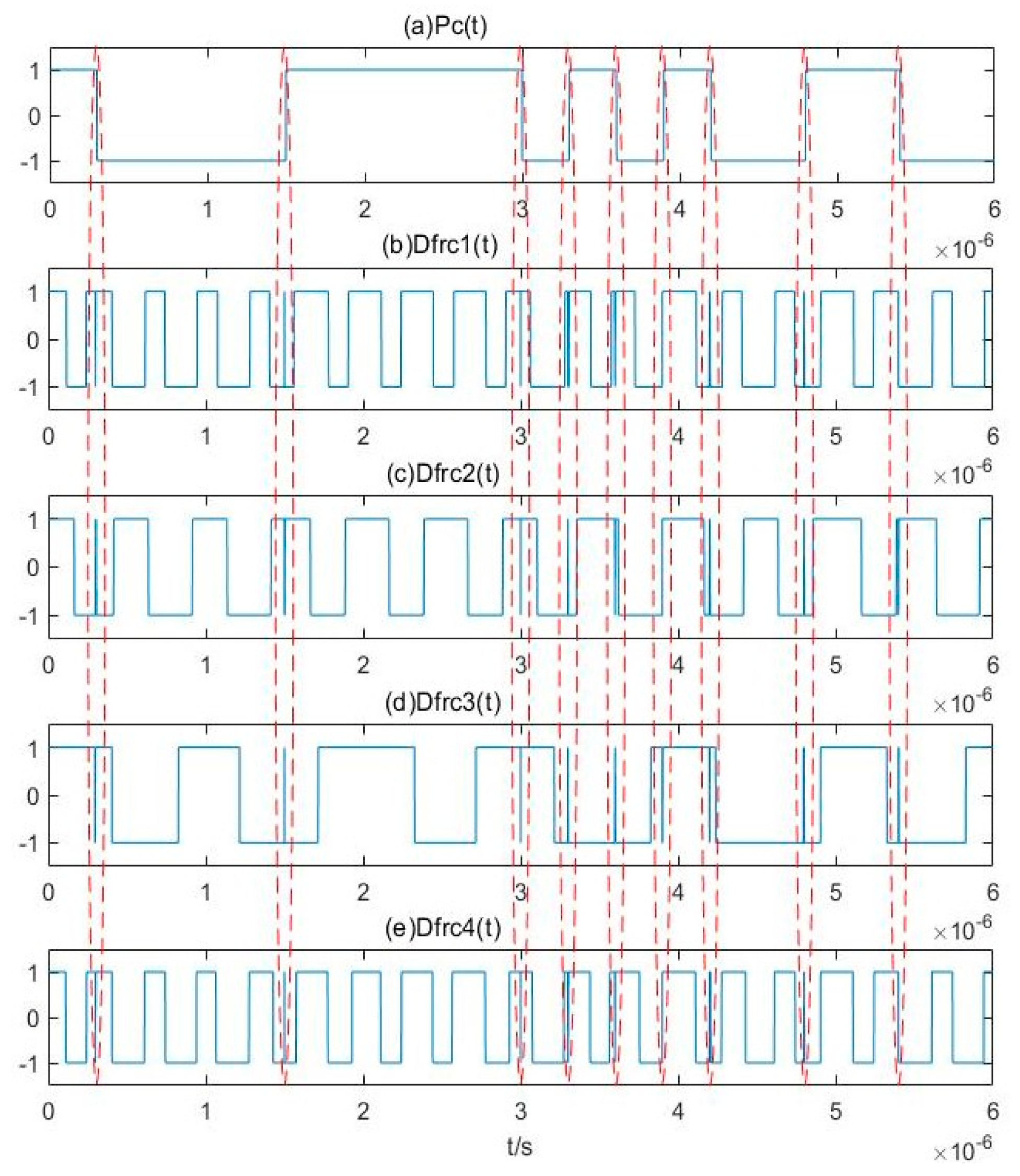
3.2. Parameter Estimation Method for BPSK Signals Based on Pilot Frequency Array Synchronization

In a weak signal detection system, the use of a Duffing oscillator array is of great importance in many ways. By setting different internal driving force signals for each Duffing oscillator, the array can achieve multiply frequency measuring ranges and increased detection and estimation precision while eliminating the phase and frequency of blind areas.

When BPSK signals pass the Duffing oscillator array with different internal driving force signals, each oscillator output corresponding to different intermittent chaos period. However, all the oscillators are controlled by the same phase code φ_i, the states of them will change at the same time. Therefore, the intermittent chaos states of array have a certain regularity, which can be used for the blind estimation of pseudo random sequences.

For each Duffing oscillator array, the internal driving force signal is ${\gamma }_{\mathrm{r}}\cos ({\omega }_{j}t)$. At this time, the binarization cosine function of the frequency difference between the internal driving force signal and the BPSK signal Df(t) varies with the frequency of the internal driving force signal

$$\mathrm{D}{f}_j(t)=\{\begin{array}{c}1\\ -1\end{array}\begin{array}{c},\\ ,\end{array}\begin{array}{c}\mathrm{sgn}(\cos (\mathsf{\Delta }{\omega }_{j}t+{\phi }_0))=1\\ \mathrm{else}\end{array}$$

(17)

After inputting the BPSK signal, the output characteristics are converted into binary Sys_j(t). Taking a simple array of two Duffing oscillators as an example, the binarization of the output characteristics Sys₁(t) and Sys₂(t) involves numerical conversion between 1 and –1 simultaneously affected by Pc(t), Df₁(t), and Df₂(t). Due to the difference in the period of Df₁(t) and Df₂(t), the time-domain waveforms of Sys₁(t) and Sys₂(t) are quite different. However, as the time of the output state transformation caused by Pc(t) in each Duffing oscillator in the array is always the same, there will always be a time when the numerical transformation occurs synchronously in Sys₁(t) and Sys₂(t). This time corresponds to the numerical transformation in Pc(t), as shown in Figure 12. Figure 12a is the pseudo-random sequence Pc(t). Figure 12b,c show the binarization results of Sys₁(t) and Sys₂(t) obtained after the BPSK signal modulated by Pc(t) has passed through two different Duffing oscillators in the array. The synchronous numerical transformations are marked with red ellipses, and these are consistent with the jump law of Pc(t). This constitutes the array synchronization of the output characteristics of the Duffing oscillator for the BPSK signals. The array synchronization obtained through the Duffing oscillator array with different frequencies is called pilot frequency array synchronization.

According to this property, we can input the BPSK signal into a group of Duffing oscillator arrays that have different internal driving force signals with different frequencies. After obtaining the binarization output characteristics, we can determine the position at which the numerical conversion takes place synchronously according to the array synchronization and obtain Pc(t). Subsequently, we can calculate the Df_i(t) of the array according to Equation (12). Averaging Df_i(t), we then obtain the estimated carrier frequency Df(t). For a pilot frequency Duffing oscillator array, because the frequency range of a single oscillator is about 0.03 ω, we set the frequency difference between each oscillator and the center frequency ω to be less than 0.03 ω.

We take the pilot frequency Duffing array as an example and propose a parameter estimation method for BPSK signals based on the synchronization of the array, as shown in Figure 13. As in Figure 9, we can get Sys_j(t) after binaryzation of the state identification of Duffing oscillator array excited by the unknown BPSK signal. Then the pseudo-random sequence can be estimated by the pilot frequency array synchronization of Duffing oscillators. After obtaining Df_i(t) based on the multiplication formula in Equation (13), we can complete the estimation of the carrier frequency.

According to the parameter estimation method in Figure 13, the carrier frequency and pseudo-random sequence of the BPSK signal in Figure 3 can be estimated. The signal to be detected is processed through an array formed by four Duffing oscillators with internal driving force frequencies of 97 MHz (oscillator 1), 98 MHz (oscillator 2), 101 MHz (oscillator 3), and 103 MHz (oscillator 4). The output of this system is shown in Figure 14.

After binarizing this array, the pseudo-random sequence estimation can be obtained based on pilot frequency synchronization. The results are shown in Figure 15.

The cosine function of binarized frequency difference obtained from the Duffing oscillator array according to Equation (12) is shown in Figure 16. As for the analysis of Figure 11, the arrows in this figure represent the time at which the value of the pseudo-random sequence shown in Figure 15e changes. If two state changes occur in the vicinity of this time within a relatively short period, they will be eliminated at the same time, and the estimated results after deburring can be obtained, as shown in Figure 17.

The frequencies of four Duffing oscillators as shown in Figure 17. The frequency differences between Duffing oscillators 1~4 and the center frequency are approximately 3.02816 MHz, 2.02925 MHz, 1.02999 MHz, and 3.03061 MHz, respectively. Therefore, the estimated center frequency based on these four oscillators are 100.02816 MHz, 100.02925 MHz, 99.97001 MHz, and 99.96939 MHz. The average value is 99.9992 MHz, with an error of only 0.0008%. These results show that the proposed method can estimate the signal parameters effectively.

4. Experimental Validation Using the BPSK Signal Parameter Estimation Method

4.1. Simulation Experiment

To verify the feasibility of the two parameter estimation methods for BPSK signal, their performance in a Duffing oscillator weak signal detection system needs to be investigated. Thus, experiments were conducted to examine the estimation accuracy of the carrier frequency and the similarity of pseudo-random sequences under various SNRs. As a performance reference, the pseudo-random sequence was also estimated directly based on the known carrier frequency.

As in the simulation described in Section 3, the carrier frequency of the to-be-detected BPSK signal is 100 MHz, the symbol width of pseudo-random sequence is 300 ns, and signal amplitude is 0.6. The two-way Duffing oscillators adopted for the Duffing oscillator array based on implied periodicity have internal driving force frequencies of 103 MHz and 98 MHz. The Duffing oscillator array based on pilot frequency array synchronism is composed of four different Duffing oscillators with frequencies of 97 MHz, 98 MHz, 101 MHz, and 103 MHz, respectively. For the Duffing oscillator with the known carrier frequency, the driving force frequency is 100 MHz. The dynamic amplitudes of all dynamic amplitudes of Duffing oscillators are set to be close to the critical value, that is, γ_r = 0.826. These parameters are shown in

Table 2. Simulation parameters.

	Methods	Implied Periodicity	Pilot Frequency Array Synchronism
Parameters
Duffing oscillator	a	1	1
	b	1	1
	k	0.5	0.5
	Amplitude	0.826	0.826
	Frequency	103 MHz, 98 MHz	97 MHz, 98 MHz, 101 MHz, 103 MHz
BPSK signal	Code Width	30 ns	30 ns
	Amplitude	0.6	0.6
	Frequency	100 MHz	100 MHz

.

BPSK signal detection under different SNR is realized by adjusting Gaussian noise variance σ². To produce SNR = −10 dB, −20 dB, −30 dB, and −35 dB, we set σ² to be 1.8, 18, 180, and 569.21, respectively. Under such conditions, the pseudo-random sequences obtained by the three methods are shown in Figure 18, Figure 19, Figure 20 and Figure 21. According to Figure 18 and Figure 19, when the SNR is −10 dB or −20 dB, the three methods all obtain good pseudo-random sequence estimation results. As SNR decreases, the difference between the chaotic state and the large-scale periodic state becomes smaller, and the identification becomes more difficult. Figure 20 and Figure 21 show the gradual appearance of several burrs that are difficult to remove. However, although the carrier frequency of the BPSK signal is unknown, the accuracy of the two blind estimation methods proposed in this paper approaches that of the traditional parameter estimation method with known carrier frequency. The pseudo-random sequence estimation also achieves good accuracy under the −35 dB SNR.

In parameter estimation, the correlation similarity coefficient is widely used to characterize the estimation accuracy of the pseudo-random sequence. This is the ratio of the peak value of the cross-correlation function between the obtained pseudo-random sequence and the original sequence to the peak value of the autocorrelation function of the original sequence.

Table 3. Simulation results of pseudo-random sequence correlation similarity coefficients at different SNR.

SNR/dB	Correlation Similarity Coefficients
	Based on Implied Periodicity	Based on Array Synchronization	Based on Known Carrier Frequency
−10	0.9627	0.9725	0.9740
−20	0.9543	0.9703	0.9683
−30	0.9470	0.9627	0.9604
−35	0.9120	0.9156	0.9230
−40	0.8205	0.8208	0.8231

presents the correlation similarity coefficients between the obtained pseudo-random sequences and the original sequences estimated by the three methods at different SNR. The pseudo-random sequences estimated by the three methods under −35 dB all have good cross-correlation performance with respect to the original sequence (correlation similarity coefficient >0.9). Relatively speaking, when the SNR is relatively high, the BPSK signal parameter estimation method based on array synchronization is closer to (and sometimes even better than) the estimation result of the special case in which the carrier frequency is known. When SNR is less than −35 dB, the correlation similarity coefficients obtained by the three methods decrease and take similar values.

The carrier frequency estimation results of the two parameter estimation methods proposed in the paper at different SNR are shown in

Table 4. Simulation results under different SNR.

SNR/dB	Carrier Frequency Estimation Relative Error (%)
	Based on Implied Periodicity	Based on Array Synchronization
−10	0.0101	0.0142
−20	0.0112	0.0327
−30	0.0355	0.0491
−35	0.0828	0.0895
−40	0.2470	0.2794

. Under an SNR of −35 dB, the parameter estimation methods based on implicit periodicity and array synchronization achieve high precision. Parameter estimation method based on the implicit periodicity produces more accurate carrier frequency estimations. This probably because the implicit periodicity method estimates carrier frequency directly, whereas array synchronization first estimates the pseudo-random sequence, and then performs additional multiplication operations to get the carrier frequency, which will produce more errors.

The simulation results show that the two parameter estimation methods proposed in this paper for the detection of weak BPSK signals based on the Duffing oscillator system can achieve high precision under −35 dB SNR. Under the condition of an unknown carrier frequency, these methods achieve similar estimation precision to the traditional approach in which the carrier frequency is known.

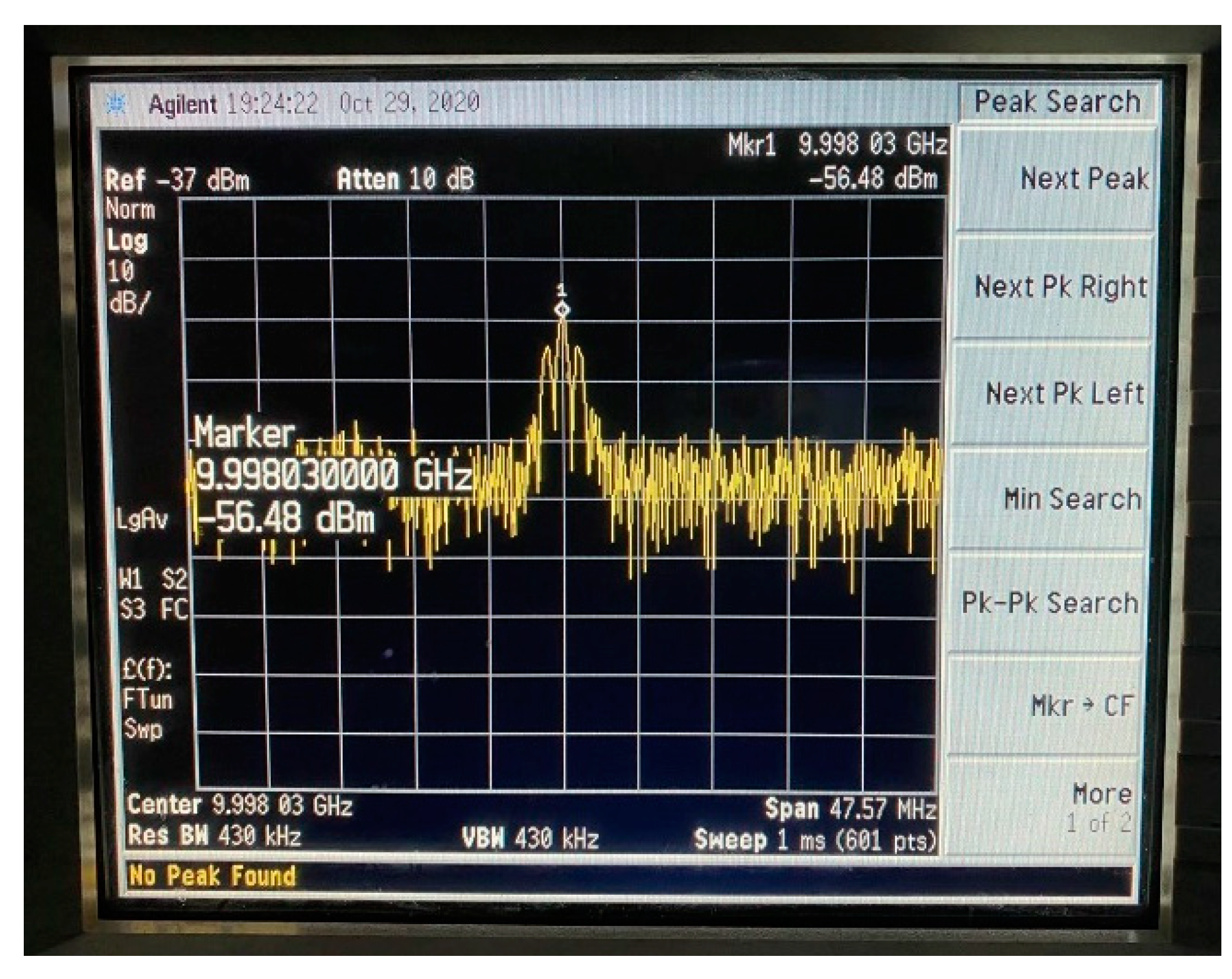
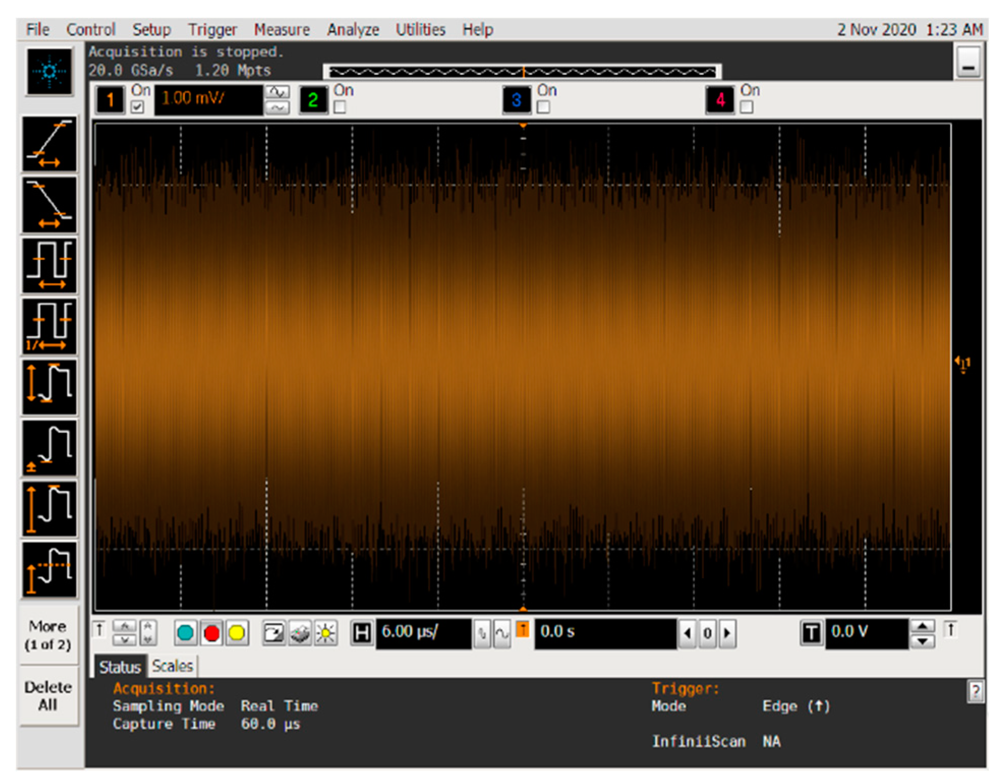
4.2. Semi-physical Simulation Experiment

In order to realize the blind parameter estimation verification of BPSK signal based on Duffing oscillator, a semi-physical experiment system was established. A BPSK signal can be sent by the pseudo-random code phase modulation prototype and received by an antenna. After down-conversion, the signal with intermediate frequency is fed into the computer and estimated by Duffing oscillator system. Subsequently, the BPSK signal can be reconstruct according to the detected parameters. Finally, we test the effect of parameter estimation by correlative processing between the received intermediate frequency signal and the reconstructed one. Images of spectrum of emitted BPSK signal, time-domain of the signal after down-conversion, time-domain of the reconstructed signals based on Duffing oscillator methods and the experiment result of correlation processing are provided in Figure 22, Figure 23, Figure 24, Figure 25 and Figure 26.

According to Figure 22, the frequency of emitted BPSK signal is approximately 10 GHz. We down-convert it to adjust the frequency to 100 MHz. The pseudo-random sequence of the emitted BPSK signal can be expressed as 100000111010110111110001010010 over a period of 6 × 10^–6 s. As shown in Figure 23, each place where the phase flips represents a change in the pseudo-random sequence. After parameter estimation based on Duffing oscillator implied periodicity and pilot frequency array synchronization, the estimated carrier frequencies are 99.992 MHz and 99.9873 MHz, respectively. The estimated pseudo-random sequences and reconstructed BPSK signals obtained by these two Duffing oscillator methods are presented in Figure 24 and Figure 25. As shown in Figure 26, the maximum correlation coefficient based on two Duffing oscillator methods between the received signal and the reconstructed signal is 0.9401 and 0.9351, respectively, which proves the validity of these two methods.

5. Conclusions

In this letter, we have analyzed the output characteristics of BPSK signals through the Duffing oscillator and derived the multiplication relationship among the output of the Duffing oscillator, pseudo-random sequence, and cosine of the difference frequency, providing a theoretical basis for the blind estimation of BPSK signal. Based on it, we propose two blind estimation methods. Simulation and experiment results show that these two methods can estimate pseudo-random sequences and carrier frequencies with high accuracy and offer strong performance when SNR = –35 dB.

However, in our methods, pseudo-random sequences and carrier frequencies are closely related, if one parameter estimation has an error, it affects the other. Small errors have great effect on the estimation results. In addition, the binarization precision of the Duffing oscillator output signal in this paper is not high. In the future, we need to find a method to distinguish chaotic states in intermittent chaotic state of Duffing oscillator with less error, which can improve the overall estimation accuracy.

References

1. Hannen, P. Radar and Electronic Warfare Principles for the Non-specialist. In Radar Electronic Warfare Principles for the Non-Specialist; Scitech Publishing: Raleigh, NC, USA, 2013. [Google Scholar]
2. Golden, A., Jr. Radar Electronic Warfare; American Institute of Aeronautics and Astronautics (AIAA): Washington, DC, USA, 1987; ISBN 10 2514 4 403225. [Google Scholar]
3. Hu, Y.; Sawan, M. A fully integrated low-power BPSK demodulator for implantable medical devices. IEEE Trans. Circuits Syst. I Regul. Pap. 2005, 52, 2552–2562. [Google Scholar] [CrossRef]
4. Nabovati, G.; Maymandi-Nejad, M. Ultra-low power BPSK demodulator for bio-implantable chips. IEICE Electron. Express 2010, 7, 1592–1596. [Google Scholar] [CrossRef] [Green Version]
5. Luo, Z.; Sonkusale, S. A Novel BPSK Demodulator for Biological Implants. IEEE Trans. Circuits Syst. I Regul. Pap. 2008, 55, 1478–1484. [Google Scholar] [CrossRef]
6. Nguyen, V.D.; Luong, N.S.; Patzold, M. A method to estimate the path gains and propagation delays of underwater acoustic channels using the arrival phase information of the multipath components. AEU Int. J. Electron. Commun. 2017, 73, 129–138. [Google Scholar] [CrossRef]
7. Jin, Y.; Ji, H. Cyclic Statistic Based Blind Parameter Estimation of BPSK and QPSK Signals. In Proceedings of the 2006 8th International Conference on Signal Processing, Guilin, China, 16–20 November 2006; Institute of Electrical and Electronics Engineers (IEEE): New York, NY, USA, 2006; Volume 1, ISBN 10 1109 2006 344452. [Google Scholar]
8. Yang, W.; Yang, X.; Kuang, Y. Research on parameter estimation of MPSK signals based on the generalized second-order cyclic spectrum. In Proceedings of the 2014 XXXIth URSI General Assembly and Scientific Symposium (URSI GASS), Beijing, China, 16–23 August 2014. [Google Scholar] [CrossRef]
9. Zhan, Y.; Duan, C. The application of stochastic resonance in parameter estimation for PSK signals. In Proceedings of the 2015 IEEE International Conference on Communication Software and Networks (ICCSN), Chengdu, China, 6–7 June 2015; Institute of Electrical and Electronics Engineers (IEEE): New York, NY, USA, 2015; pp. 166–172. [Google Scholar]
10. Wang, Q.; Ge, Q. Blind estimation algorithm of parameters in PN sequence for DSSS-BPSK signals. In Proceedings of the 2012 International Conference on Wavelet Active Media Technology and Information Processing (ICWAMTIP), Chengdu, China, 17–19 December 2012; Institute of Electrical and Electronics Engineers (IEEE): New York, NY, USA, 2012; pp. 371–376. [Google Scholar]
11. Guolin, L.; Min, H.; Ying, Z. PN Code Recognition and Parameter Estimation of PN-BPSK Signal Based on Synchronous Demodulation. In Proceedings of the 2007 8th International Conference on Electronic Measurement and Instruments, Xian, China, 16–18 August 2007; Institute of Electrical and Electronics Engineers (IEEE): New York, NY, USA, 2007; pp. 2–145. [Google Scholar]
12. Gardner, W.; Spooner, C. Detection and source location of weak cyclostationary signals: Simplifications of the maximum-likelihood receiver. IEEE Trans. Commun. 1993, 41, 905–916. [Google Scholar] [CrossRef]
13. Gardner, W.A.; Chen, C.-K. Signal-selective time-difference-of-arrival estimation for passive location of man-made signal sources in highly corruptive environments. I. Theory and method. IEEE Trans. Signal Process. 1992, 40, 1168–1184. [Google Scholar] [CrossRef]
14. Akilli, M.; Yilmaz, N. Study of Weak Periodic Signals in the EEG Signals and Their Relationship with Postsynaptic Potentials. IEEE Trans. Neural Syst. Rehabil. Eng. 2018, 26, 1918–1925. [Google Scholar] [CrossRef] [PubMed]
15. Vahedi, H.; Gharehpetian, G.B.; Karrari, M. Application of Duffing Oscillators for Passive Islanding Detection of Inverter-Based Distributed Generation Units. IEEE Trans. Power Deliv. 2012, 27, 1973–1983. [Google Scholar] [CrossRef]
16. Rashtchi, V.; Nourazar, M. FPGA Implementation of a Real-Time Weak Signal Detector Using a Duffing Oscillator. Circuits Syst. Signal Process. 2015, 34, 3101–3119. [Google Scholar] [CrossRef]
17. Patel, V.N.; Tandon, N.; Pandey, R.K. Defect detection in deep groove ball bearing in presence of external vibration using envelope analysis and Duffing oscillator. Measurement 2012, 45, 960–970. [Google Scholar] [CrossRef]
18. Wang, G.Y.; Chen, D.J.; Lin, J.Y.; Chen, X. The application of chaotic oscillators to weak signal detection. IEEE Trans. Ind. Electron. 1999, 46, 440–444. [Google Scholar] [CrossRef]
19. Liu, H.B.; Wu, D.W.; Yuan, Y.Y.; Yan, Z.J. New method for long-period DSSS/BPSK satellite signal carrier detection and power estimation. Syst. Eng. Electron. 2013, 7, 7. (In Chinese) [Google Scholar]
20. Hu, J.; Wang, K. Carrier Detection Method of Binary-Phase-Shift-Keyed and Direct-Sequence-Spread-Spectrum Signals Based on Duffing Oscillator. Int. Conf. Telecommun. 2006, 1338–1341. [Google Scholar] [CrossRef]
21. Zhang, S.; Rui, G.S. Chaotic detector for BPSK signals in very low SNR conditions. Int. J. Bifurc. Chaos 2012, 22, 1250144. [Google Scholar] [CrossRef]
22. Fu, Y.Q.; Wu, D.M.; Zhang, L.; Li, X.Y. A circular zone partition method for identifying Duffing oscillator state transition and its application to BPSK signal demodulation. Sci. China Inf. Sci. 2011, 54, 1274–1282. [Google Scholar] [CrossRef]
Figure 1. Output time domain waveform of the Duffing oscillator excited by a sinusoidal signal.
Sensors 20 06412 g001
Figure 2. Output time domain waveform of the Duffing oscillator excited by binary phase shift keying (BPSK) signal.
Sensors 20 06412 g002
Figure 3. Time-domain waveforms of (a) φi; (b) cos(Δωt + φ0); (c) y(t).
Sensors 20 06412 g003
Figure 4. Time-domain waveforms of (a) Pc(t); (b) Df(t); (c) Sys(t).
Sensors 20 06412 g004
Figure 5. Vector diagram of amplitude of equivalent driving force under the action of BPSK signal: (a) before the change, γe > γc; (b) before the change, γe < γc.
Sensors 20 06412 g005
Figure 6. Vector diagram of movement rule under the action of BPSK signal: (a) before the change of φi; (b) after the change of φi.
Sensors 20 06412 g006
Figure 7. Numerical variation relationship of Sys(t) and Df(t).
Sensors 20 06412 g007
Figure 8. The points of adjacent segments.
Sensors 20 06412 g008
Figure 9. Flow diagram of the parameter estimation method based on the implied periodicity.
Sensors 20 06412 g009
Figure 10. Time-domain graph of key nodes in pseudo-random sequence estimation based on implied periodicity: (a) y(t); (b) Sys(t); (c) Dfrc(t); (d) Pcrc(t).
Sensors 20 06412 g010
Figure 11. Deburring method of Pcrc(t).
Sensors 20 06412 g011
Figure 12. Pilot frequency array synchronization of the output characteristics of Duffing oscillator.
Sensors 20 06412 g012
Figure 13. Flow diagram of the parameter estimation method for BPSK signal based on pilot frequency array synchronization of the Duffing oscillator.
Sensors 20 06412 g013
Figure 14. Output of the Duffing oscillator array: (a) oscillator 1; (b) oscillator 2; (c) oscillator 3; (d) oscillator 4.
Sensors 20 06412 g014
Figure 15. Output of the binarized Duffing oscillator array and estimation results of the pseudo-random sequence.
Sensors 20 06412 g015
Figure 16. Cosine function of binarized difference frequency of Duffing oscillator array.
Sensors 20 06412 g016
Figure 17. Estimated results after deburring: (a) Df1(t); (b) Df2(t); (c) Df3(t); (d) Df4(t).
Sensors 20 06412 g017
Figure 18. Pseudo-random sequence estimation results based on three methods with SNR = –10 dB: (a) based on implied periodicity; (b) based on pilot frequency array synchronization; (c) based on known carrier frequency.
Sensors 20 06412 g018
Figure 19. Pseudo-random sequence estimation results based on three methods with signal-to-noise ratio (SNR) = –20 dB: (a) based on implied periodicity; (b) based on pilot frequency array synchronization; (c) based on known carrier frequency.
Sensors 20 06412 g019
Figure 20. Pseudo-random sequence estimation results based on three methods with SNR = −30 dB: (a) based on implied periodicity; (b) based on pilot frequency array synchronization; (c) based on known carrier frequency.
Sensors 20 06412 g020
Figure 21. Pseudo-random sequence estimation results based on three methods with SNR = −35 dB: (a) based on implied periodicity; (b) based on pilot frequency array synchronization; (c) based on known carrier frequency.
Sensors 20 06412 g021
Figure 22. Spectrum diagram of emitted BPSK signal.
Sensors 20 06412 g022
Figure 23. Time-domain diagram of emitted BPSK signal after down-conversion.
Sensors 20 06412 g023
Figure 24. Estimated result based on Duffing oscillator implied periodicity: (a) pseudo-random sequence; (b) reconstructed BPSK signal.
Sensors 20 06412 g024
Figure 25. Estimated results based on Duffing oscillator array synchronization: (a) pseudo-random sequence; (b) reconstructed BPSK signal.
Sensors 20 06412 g025
Figure 26. Correlated results: (a) implied periodicity; (b) pilot frequency array synchronization.
Sensors 20 06412 g026