LoRa Sensor Network Development for Air Quality Monitoring or Detecting Gas Leakage Events

 ,
,  ,
,  ,
, 
Abstract
1. Introduction
2. System Design and Implementation
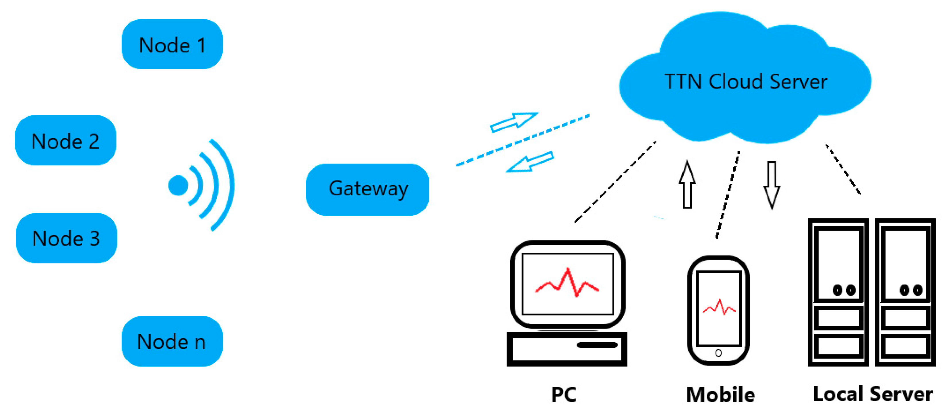
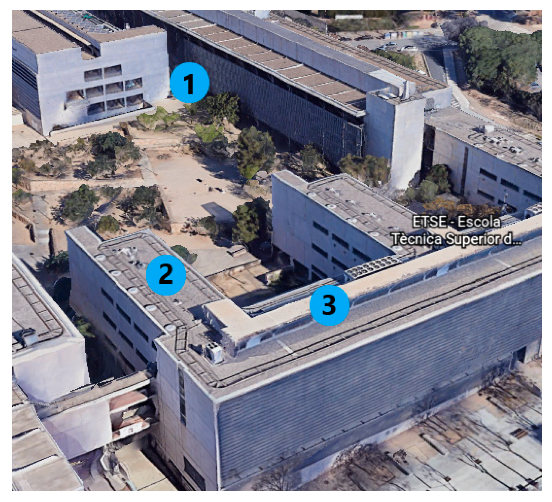
2.1. Network Deployment
2.2. Gateway
2.3. End Nodes Design and Programming
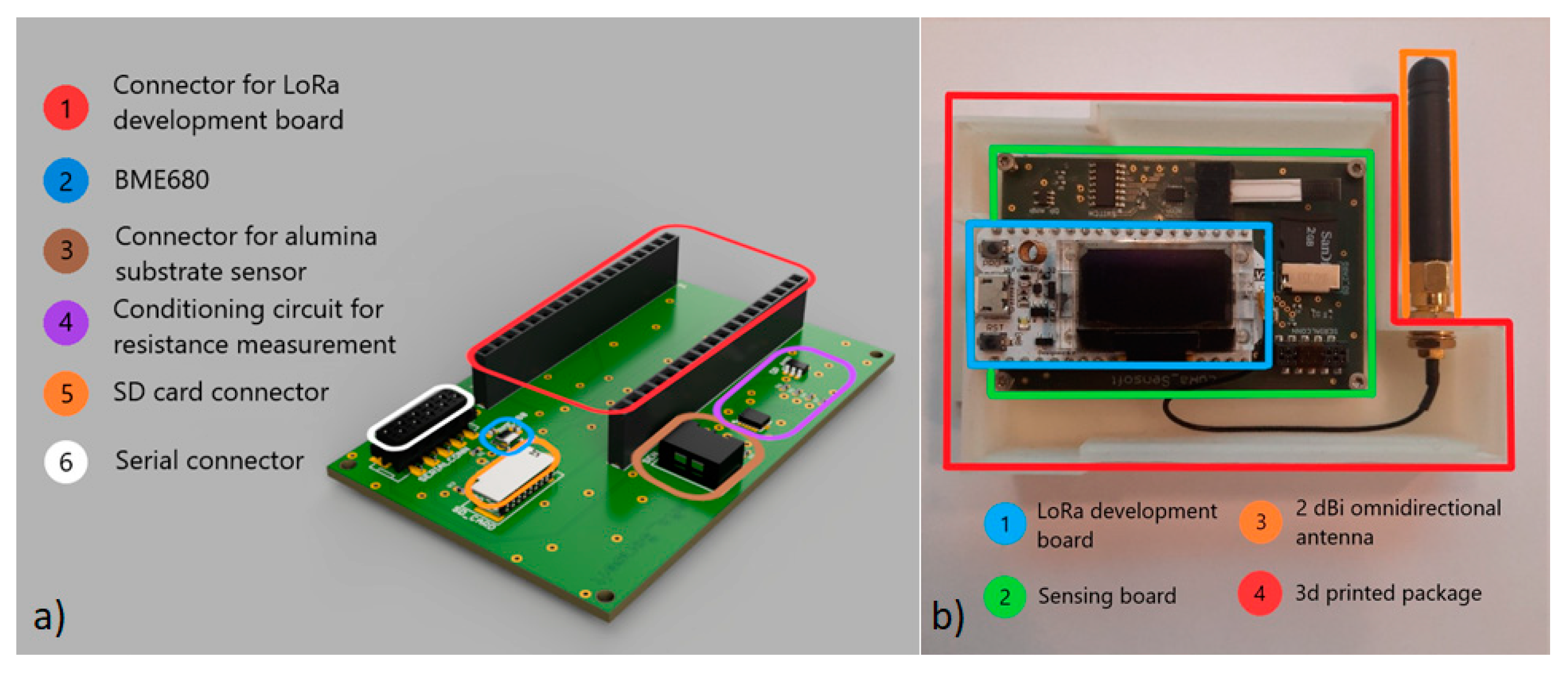
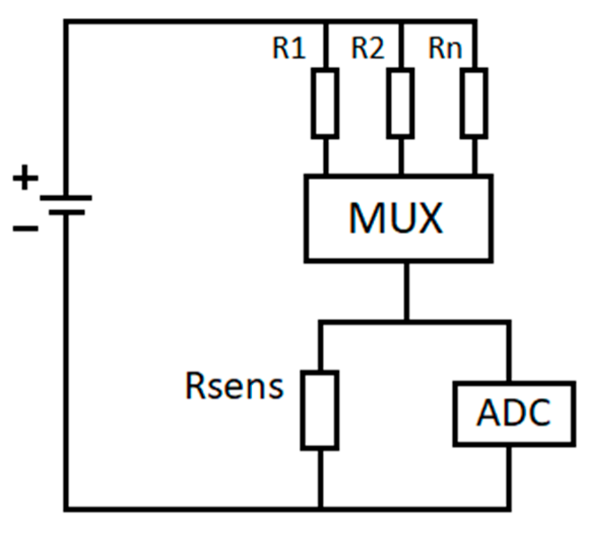
2.3.1. Hardware
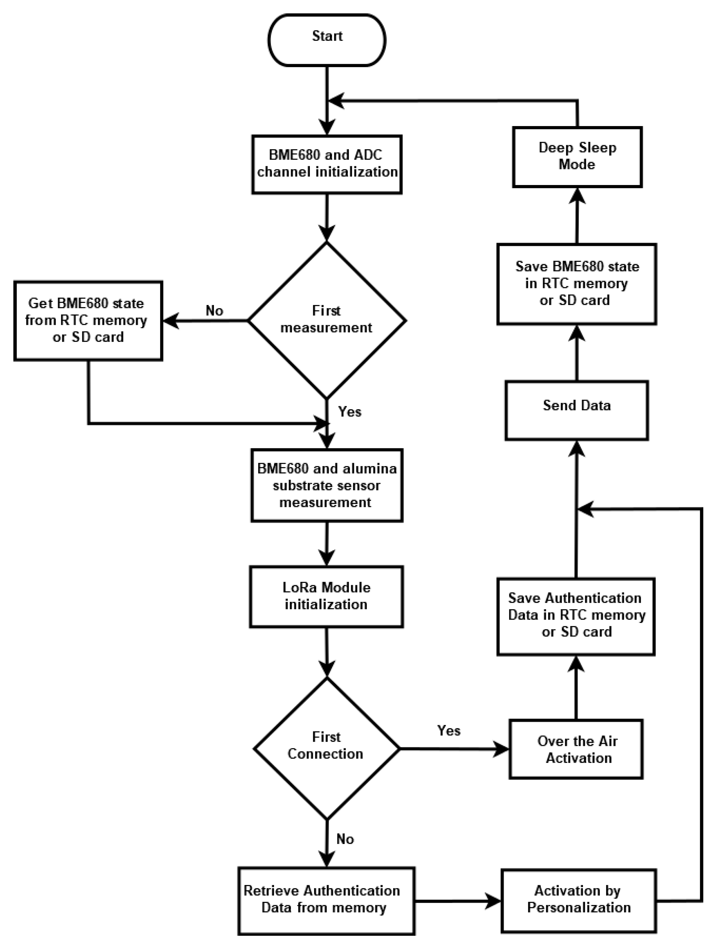
2.3.2. Software
2.4. TTN Application Server
2.5. Front-End Application
3. Graphene Sensor
3.1. Sensor Fabrication
3.2. Characterisation Techniques
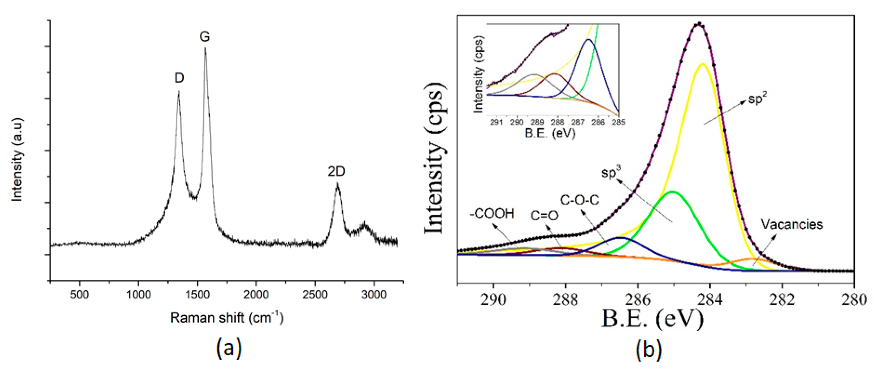
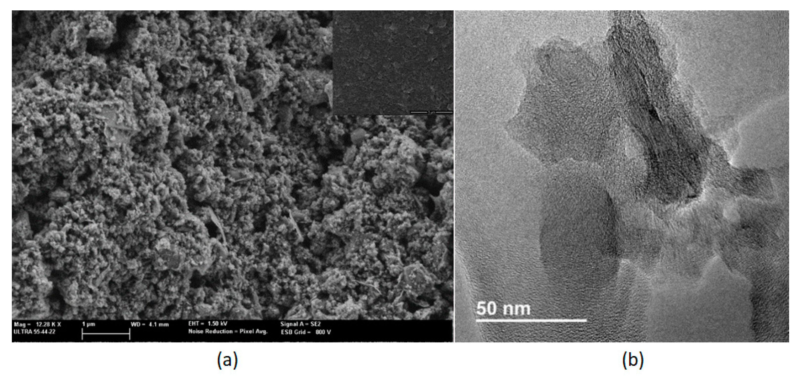
3.3. Graphene Characterisation
3.4. Gas Sensing System
3.5. Gas Sensing Mechanisms
4. Discussion
4.1. Network Performance
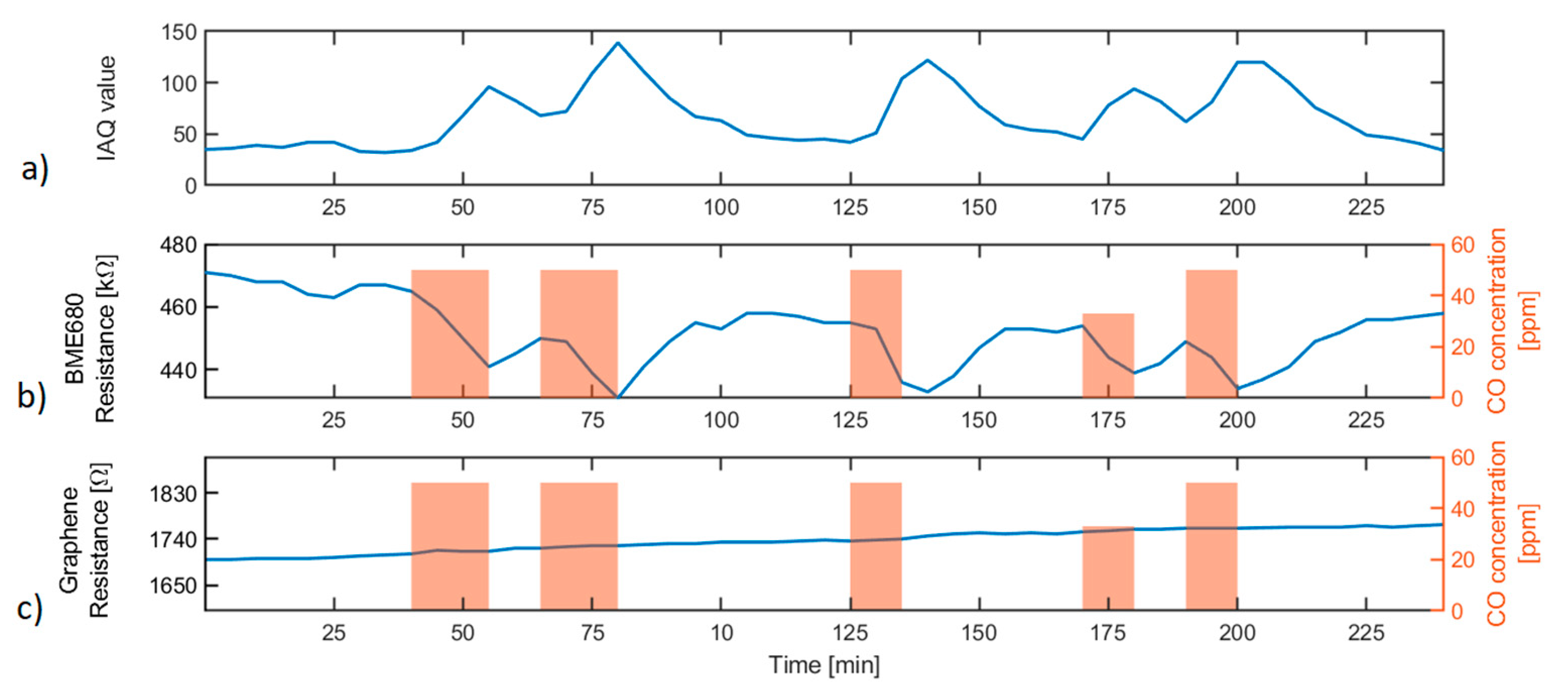
4.2. Gas Sensing Performance
5. Conclusions
Supplementary Materials
Author Contributions
Funding
Acknowledgments
Conflicts of Interest
References
- World Health Statistics 2019: Monitoring Health for the SDGs: Sustainable Development Goals; World Health Organisation: Geneva, Switzerland, 2019.
- Kumar, A.; Singh, I.P.; Sud, S.K. Energy efficient air quality monitoring system. Proc. IEEE Sens. 2011, 1562–1566. [Google Scholar] [CrossRef]
- Kim, J.Y.; Chu, C.H.; Shin, S.M. ISSAQ: An integrated sensing systems for real-time indoor air quality monitoring. IEEE Sens. J. 2014, 14, 4230–4244. [Google Scholar] [CrossRef]
- Chen, Y.Y.; Sung, F.C.; Chen, M.L.; Mao, I.F.; Lu, C.Y. Indoor air quality in the metro system in north Taiwan. Int. J. Environ. Res. Public Health 2016, 13, 1200. [Google Scholar] [CrossRef] [PubMed]
- Marques, G.; Pires, I.M.; Miranda, N.; Pitarma, R. Air quality monitoring using assistive robots for ambient assisted living and enhanced living environments through internet of things. Electron 2019, 8, 1375. [Google Scholar] [CrossRef]
- Serrano-Jiménez, A.; Lizana, J.; Molina-Huelva, M.; Barrios-Padura, Á. Indoor environmental quality in social housing with elderly occupants in Spain: Measurement results and retrofit opportunities. J. Build. Eng. 2020, 30. [Google Scholar] [CrossRef]
- Farzad, K.; Khorsandi, B.; Khorsandi, M.; Bouamra, O.; Maknoon, R. A study of cardiorespiratory related mortality as a result of exposure to black carbon. Sci. Total Environ. 2020, 725, 138422. [Google Scholar] [CrossRef]
- Ginsberg, G.M.; Kaliner, E.; Grotto, I. Mortality, hospital days and expenditures attributable to ambient air pollution from particulate matter in Israel. Isr. J. Health Policy Res. 2016, 5, 1–7. [Google Scholar] [CrossRef] [PubMed]
- Valentino, S.; Tarrade, A.; Chavatte-Palmer, P. Exposition aux gaz d’échappement diesel durant la gestation: Quelles conséquences sur le développement fœto-placentaire? Apport des modèles animaux. Bull. Acad. Vet. Fr. 2016, 208. [Google Scholar] [CrossRef]
- Pan American Health Organization. Available online: www.paho.org/en/topics/air-quality (accessed on 20 May 2020).
- Chen, X.; Wang, T.; Qiu, X.; Que, C.; Zhang, H.; Zhang, L.; Zhu, T. Susceptibility of individuals with chronic obstructive pulmonary disease to air pollution exposure in Beijing, China: A case-control panel study (COPDB). Sci. Total Environ. 2020, 717, 137285. [Google Scholar] [CrossRef]
- Effatpanah, M.; Effatpanah, H.; Jalali, S.; Parseh, I.; Goudarzi, G.; Barzegar, G.; Geravandi, S.; Darabi, F.; Ghasemian, N.; Mohammadi, M.J. Hospital admission of exposure to air pollution in Ahvaz megacity during 2010–2013. Clin. Epidemiol. Glob. Health 2019, 8, 550–556. [Google Scholar] [CrossRef]
- World Health Organiaztion. Available online: www9.who.int/airpollution/en/ (accessed on 20 May 2020).
- EPA. Indoor Air Quality|EPA’s Report on the Environment (ROE)|US EPA. Available online: https://www.epa.gov/report-environment/indoor-air-quality (accessed on 19 October 2020).
- Wilbur, S.; Williams, M.; Williams, R.; Scinicariello, F.; Klotzbach, J.M.; Diamond, G.L.; Citra, M. Toxicological profile for carbon monoxide. Available online: https://pubmed.ncbi.nlm.nih.gov/23946966/ (accessed on 31 October 2020).
- EPA. Basic Information about NO2|Nitrogen Dioxide (NO2) Pollution|US EPA. Available online: https://www.epa.gov/no2-pollution/basic-information-about-no2 (accessed on 19 October 2020).
- EPA. Quantitative Risk and Exposure Assessment for Carbon Monoxide—Amended. Available online: https://www3.epa.gov/ttn/naaqs/standards/co/data/CO-REA-Amended-July2010.pdf (accessed on 31 October 2020).
- EPA. Volatile Organic Compounds’ Impact on Indoor Air Quality|Indoor Air Quality (IAQ)|US EPA. Available online: https://www.epa.gov/indoor-air-quality-iaq/volatile-organic-compounds-impact-indoor-air-quality (accessed on 19 October 2020).
- Maag, B.; Zhou, Z.; Thiele, L. Monitoring Deployments. IEEE Internet Things J. 2018, 5, 4857–4870. [Google Scholar] [CrossRef]
- Idrees, Z.; Zheng, L. Low cost air pollution monitoring systems: A review of protocols and enabling technologies. J. Ind. Inf. Integr. 2020, 17, 100123. [Google Scholar] [CrossRef]
- Aberilla, J.M.; Gallego-Schmid, A.; Stamford, L.; Azapagic, A. Environmental sustainability of cooking fuels in remote communities: Life cycle and local impacts. Sci. Total Environ. 2020, 713, 136445. [Google Scholar] [CrossRef]
- Ometov, A.; Bezzateev, S.; Voloshina, N.; Masek, P.; Komarov, M. Environmental monitoring with distributed mesh networks: An overview and practical implementation perspective for urban scenario. Sensors 2019, 19, 5548. [Google Scholar] [CrossRef] [PubMed]
- Brzozowski, K.; Maczyński, A.; Ryguła, A. Monitoring road traffic participants’ exposure to PM10 using a low-cost system. Sci. Total Environ. 2020, 728. [Google Scholar] [CrossRef]
- Popoola, O.A.M.; Carruthers, D.; Lad, C.; Bright, V.B.; Mead, M.I.; Stettler, M.E.J.; Saffell, J.R.; Jones, R.L. Use of networks of low cost air quality sensors to quantify air quality in urban settings. Atmos. Environ. 2018, 194, 58–70. [Google Scholar] [CrossRef]
- Perez, A.O.; Bierer, B.; Scholz, L.; Wöllenstein, J.; Palzer, S. A wireless gas sensor network to monitor indoor environmental quality in schools. Sensors 2018, 18, 4345. [Google Scholar] [CrossRef]
- Prabakaran, P.; Manikandan, A. Carbon monoxide air quality index (AQI-Co) and seasonal trend (ST-Co) in Chennai traffic zones, India. Int. J. Mech. Prod. Eng. Res. Dev. 2019, 9, 871–878. [Google Scholar] [CrossRef]
- Polichetti, T.; Miglietta, M.L.; Alfano, B.; Massera, E.; De Vito, S.; Di Francia, G.; Faucon, A.; Saoutieff, E.; Boisseau, S.; Marchand, N.; et al. A Networked Wearable Device for Chemical Multisensing. In Proceedings of the Sensors; Andò, B., Baldini, F., Di Natale, C., Ferrari, V., Marletta, V., Marrazza, G., Militello, V., Miolo, G., Rossi, M., Scalise, L., et al., Eds.; Springer International Publishing: Cham, Germany, 2019; pp. 17–24. [Google Scholar]
- Rickerby, D.G.; Skouloudis, A.N. Nanostructured Metal Oxides for Sensing Toxic Air Pollutants. In RSC Detection Science; Royal Society of Chemistry: Cambridge, UK, 2017; Volume January-2017, pp. 48–90. [Google Scholar]
- Zappa, D.; Galstyan, V.; Kaur, N.; Munasinghe Arachchige, H.M.M.; Sisman, O.; Comini, E. “Metal oxide -based heterostructures for gas sensors”—A review. Anal. Chim. Acta 2018, 1039, 1–23. [Google Scholar] [CrossRef]
- Navarrete, E.; Bittencourt, C.; Umek, P.; Llobet, E. AACVD and gas sensing properties of nickel oxide nanoparticle decorated tungsten oxide nanowires. J. Mater. Chem. C 2018, 6, 5181–5192. [Google Scholar] [CrossRef]
- Rodner, M.; Puglisi, D.; Ekeroth, S.; Helmersson, U.; Shtepliuk, I.; Yakimova, R.; Skallberg, A.; Uvdal, K.; Schütze, A.; Eriksson, J. Graphene decorated with iron oxide nanoparticles for highly sensitive interaction with volatile organic compounds. Sensors 2019, 19, 918. [Google Scholar] [CrossRef] [PubMed]
- Oluwasanya, P.W.; Samad, Y.A.; Occhipinti, L.G. Printable sensors for Nitrogen dioxide and Ammonia sensing at room temperature. In Proceedings of the 2019 IEEE International Conference on Flexible and Printable Sensors and Systems (FLEPS), Glasgow, UK, 8–10 July 2019; pp. 2019–2021. [Google Scholar] [CrossRef]
- Sudhan, N.; Lavanya, N.; Leonardi, S.G.; Neri, G.; Sekar, C. Monitoring of chemical risk factors for sudden infant death syndrome (SIDS) by hydroxyapatite-graphene-MWCNT composite-based sensors. Sensors 2019, 19, 3437. [Google Scholar] [CrossRef]
- Peng, H.; Li, F.; Hua, Z.; Yang, K.; Yin, F.; Yuan, W. Highly sensitive and selective room-temperature nitrogen dioxide sensors based on porous graphene. Sens. Actuators B Chem. 2018, 275, 78–85. [Google Scholar] [CrossRef]
- Chen, Y.; Ghannam, R.; Heidari, H. Air Quality Monitoring using Portable Multi-Sensory Module for Neurological Disease Prevention. In Proceedings of the 2019 UK/China Emerging Technologies (UCET), Glasgow, UK, 21–22 August 2019; pp. 19–22. [Google Scholar] [CrossRef]
- Hussain, S.A.; Al Ghawi, S.; Al Rawahi, B.; Hussain, S.J. Design and implementation of indoor environment monitoring and controlling system. Int. J. Adv. Sci. Technol. 2020, 29, 8–14. [Google Scholar]
- Chojer, H.; Branco, P.T.B.S.; Martins, F.G.; Alvim-Ferraz, M.C.M.; Sousa, S.I.V. Development of low-cost indoor air quality monitoring devices: Recent advancements. Sci. Total Environ. 2020, 727, 138385. [Google Scholar] [CrossRef] [PubMed]
- Samee, I.U.; Jilani, M.T.; Wahab, H.G.A. An Application of IoT and Machine Learning to Air Pollution Monitoring in Smart Cities. In Proceedings of the 2019 4th International Conference on Emerging Trends in Engineering, Sciences and Technology (ICEEST), Karachi, Pakistan, 10–11 December 2019; pp. 2–7. [Google Scholar] [CrossRef]
- Zhao, L.; Wu, W.; Li, S. Design and Implementation of an IoT-Based Indoor Air Quality Detector With Multiple Communication Interfaces. IEEE Internet Things J. 2019, 6, 9621–9632. [Google Scholar] [CrossRef]
- Karunanithy, K.; Velusamy, B. Energy efficient Cluster and Travelling Salesman Problem based Data Collection using WSNs for Intelligent Water Irrigation and Fertigation. Measurement 2020, 161, 107835. [Google Scholar] [CrossRef]
- Saqib, M.; Almohamad, T.A.; Mehmood, R.M. A low-cost information monitoring system for smart farming applications. Sensors 2020, 20, 2367. [Google Scholar] [CrossRef]
- Difallah, W.; Bounaama, F.; Benahmed, K.; Draoui, B.; Maamar, A. Smart irrigation technology for efficient water use. In Proceedings of the 7th International Conference on Software Engineering and New Technologies, New York, NY, USA, 26–28 December 2018. [Google Scholar] [CrossRef]
- Lin, R.; Kim, H.J.; Achavananthadith, S.; Kurt, S.A.; Tan, S.C.C.; Yao, H.; Tee, B.C.K.; Lee, J.K.W.; Ho, J.S. Wireless battery-free body sensor networks using near-field-enabled clothing. Nat. Commun. 2020, 11, 1–10. [Google Scholar] [CrossRef]
- Geman, O.; Chiuchisan, I.; Ungurean, I.; Hagan, M.; Arif, M. Ubiquitous healthcare system based on the sensors network and android internet of things gateway. In Proceedings of the 2018 IEEE SmartWorld, Ubiquitous Intelligence & Computing, Advanced & Trusted Computed, Scalable Computing & Communications, Cloud & Big Data Computing, Internet of People and Smart City Innovation (SmartWorld/SCALCOM/UIC/ATC/CBDCom/IOP/SCI), Guangzhou, China, 8–12 October 2018; 2018; pp. 1390–1395. [Google Scholar] [CrossRef]
- Chatterjee, A.; Biswas, J.; Das, K. An automated patient monitoring using discrete-time wireless sensor networks. Int. J. Commun. Syst. 2020, 33, 1–14. [Google Scholar] [CrossRef]
- Gautam, S.K.; Om, H. Intrusion detection in RFID system using computational intelligence approach for underground mines. Int. J. Commun. Syst. 2018, 31, 1–24. [Google Scholar] [CrossRef]
- Almomani, I.; Alromi, A. Integrating software engineering processes in the development of efficient intrusion detection systems in wireless sensor networks. Sensors 2020, 20, 1375. [Google Scholar] [CrossRef]
- Vladuta, V.A.; Apostol, I.; Ghimes, A.M. Data Collection Analysis: Field Experiments with Wireless Sensors and Unmanned Aerial Vehicles. In Proceedings of the 2018 International Conference on Communications (COMM), Bucharest, Romania, 14–16 June 2018; pp. 529–534. [Google Scholar] [CrossRef]
- Landaluce, H.; Arjona, L.; Perallos, A.; Falcone, F.; Angulo, I.; Muralter, F. A review of iot sensing applications and challenges using RFID and wireless sensor networks. Sensors 2020, 20, 2495. [Google Scholar] [CrossRef] [PubMed]
- Awadallah, S.; Moure, D.; Torres-González, P. An internet of things (IoT) application on volcano monitoring. Sensors 2019, 19, 4651. [Google Scholar] [CrossRef] [PubMed]
- Villa-Henriksen, A.; Edwards, G.T.C.; Pesonen, L.A.; Green, O.; Sørensen, C.A.G. Internet of Things in arable farming: Implementation, applications, challenges and potential. Biosyst. Eng. 2020, 191, 60–84. [Google Scholar] [CrossRef]
- Chang, C.; Srirama, S.N.; Buyya, R. Internet of Things (IoT) and New Computing Paradigms. Fog Edge Comput. 2019, 1–23. [Google Scholar] [CrossRef]
- Xia, F.; Yang, L.T.; Wang, L.; Vinel, A. Internet of things. Int. J. Commun. Syst. 2012, 25, 1101–1102. [Google Scholar] [CrossRef]
- Zhou, H.; Li, S.; Chen, S.; Zhang, Q.; Liu, W.; Guo, X. Enabling Low Cost Flexible Smart Packaging System with Internet-of-Things Connectivity via Flexible Hybrid Integration of Silicon RFID Chip and Printed Polymer Sensors. IEEE Sens. J. 2020, 20, 5004–5011. [Google Scholar] [CrossRef]
- Devan, P.A.M.; Hussin, F.A.; Ibrahim, R.; Bingi, K.; Nagarajapandian, M. IoT Based Vehicle Emission Monitoring and Alerting System. In Proceedings of the 2019 IEEE Student Conference on Research and Development (SCOReD), Bandar Seri Iskandar, Malaysia, 15–17 October 2019; pp. 161–165. [Google Scholar] [CrossRef]
- Rustia, D.J.A.; Lin, C.E.; Chung, J.Y.; Zhuang, Y.J.; Hsu, J.C.; Lin, T. Te Application of an image and environmental sensor network for automated greenhouse insect pest monitoring. J. Asia Pac. Entomol. 2020, 23, 17–28. [Google Scholar] [CrossRef]
- Rodríguez-Robles, J.; Martin, Á.; Martin, S.; Ruipérez-Valiente, J.A.; Castro, M. Autonomous sensor network for rural agriculture environments, low cost, and energy self-charge. Sustainability 2020, 12, 5913. [Google Scholar] [CrossRef]
- Chaudhari, B.S.; Zennaro, M.; Borkar, S. LPWAN technologies: Emerging application characteristics, requirements, and design considerations. Futur. Internet 2020, 12, 46. [Google Scholar] [CrossRef]
- LoRa Alliance White Paper: A Technical Overview of LoRa and LoRaWAN. 2015. Available online: https://lora-alliance.org/resource-hub/what-lorawanr (accessed on 31 October 2020).
- LoRa Alliance Technical Commitee LoRaWAN 1.1 Specification. 2017. Available online: https://lora-alliance.org/resource-hub/lorawanr-specification-v11 (accessed on 31 October 2020).
- Van Wijnen, J.H.; Verhoeff, A.P.; Jans, H.W.A.; van Bruggen, M. The exposure of cyclists, car drivers and pedestrians to traffic-related air pollutants. Int. Arch. Occup. Environ. Health 1995, 67, 187–193. [Google Scholar] [CrossRef] [PubMed]
- Novikov, S.; Lebedeva, N.; Satrapinski, A.; Walden, J.; Davydov, V.; Lebedev, A. Graphene based sensor for environmental monitoring of NO2. Sens. Actuators B Chem. 2016, 236, 1054–1060. [Google Scholar] [CrossRef]
- Panda, D.; Nandi, A.; Datta, S.K.; Saha, H.; Majumdar, S. Selective detection of carbon monoxide (CO) gas by reduced graphene oxide (rGO) at room temperature. RSC Adv. 2016, 6, 47337–47348. [Google Scholar] [CrossRef]
- Sensortec, B. BME680 Low Power Gas, Pressure, Temperature & Humidity Sensor. 2019. Available online: https://cdn-shop.adafruit.com/product-files/3660/BME680.pdf (accessed on 31 October 2020).
- Lozano, J.; Suarez, J.I.; Melendez, F.; Rodriguez, S.; Arroyo, P.; Herrero, J.L.; Carmona, P. Personal electronic systems for citizen measurements of air quality. In Proceedings of the 2019 5th Experiment at International Conference (exp.at 2019), Funchal (Madeira Island), Portugal, 12–14 June 2019; Institute of Electrical and Electronics Engineers Inc.: Piscataway, NJ, USA, 2019; pp. 315–319. [Google Scholar]
- Jose, J.; Sasipraba, T. Indoor air quality monitors using IOT sensors and LPWAN. In Proceedings of the International Conference on Trends in Electronics and Informatics (ICOEI 2019), Tirunelveli, India, 12 March 2019; Institute of Electrical and Electronics Engineers Inc.: Piscataway, NJ, USA, 2019; Volume 2019-April, pp. 633–637. [Google Scholar]
- Lasomsri, P.; Yanbuaban, P.; Kerdpoca, O.; Ouypornkochagorn, T. A development of low-cost devices for monitoring indoor air quality in a large-scale hospital. In Proceedings of the ECTI-CON 2018—15th International Conference on Electrical Engineering/Electronics, Computer, Telecommunications and Information Technology, Chiang Rai, Thailand, 18–21 July 2018; Institute of Electrical and Electronics Engineers Inc.: Piscataway, NJ, USA, 2019; pp. 282–285. [Google Scholar]
- Thakor, G.S.N.; Hu, P.; Motisan, R.; Chiang, E.; Santos, R. Testing & validation of mobile air quality monitor for sensing & dilineating VOC emissions. In Proceedings of the Air and Waste Management Association’s Annual Conference and Exhibition, Quebec, QC, Canada, 25–28 June 2019. [Google Scholar]
- Eklund, P.C.; Holden, J.M.; Jishi, R.A. Vibrational Modes of Carbon Nanotubes; Spectroscopy and Theory; Elsevier Science Limited: Oxford, UK, 1996. [Google Scholar]
- Wu, J.B.; Lin, M.L.; Cong, X.; Liu, H.N.; Tan, P.H. Raman spectroscopy of graphene-based materials and its applications in related devices. Chem. Soc. Rev. 2018, 47, 1822–1873. [Google Scholar] [CrossRef] [PubMed]
- Jorio, A. Raman Spectroscopy in Graphene-Based Systems: Prototypes for Nanoscience and Nanometrology. ISRN Nanotechnol. 2012, 2012, 1–16. [Google Scholar] [CrossRef]
- Yang, G.; Kim, B.-J.; Kim, K.; Woo Han, J.; Kim, J. Energy and dose dependence of proton-irradiation damage in graphene. RSC Adv. 2015. [Google Scholar] [CrossRef]
- Acosta, S.; Casanova Chafer, J.; Sierra Castillo, A.; Llobet, E.; Snyders, R.; Colomer, J.-F.; Quintana, M.; Ewels, C.; Bittencourt, C. Low Kinetic Energy Oxygen Ion Irradiation of Vertically Aligned Carbon Nanotubes. Appl. Sci. 2019, 9, 5342. [Google Scholar] [CrossRef]
- Ganesan, K.; Ghosh, S.; Gopala Krishna, N.; Ilango, S.; Kamruddin, M.; Tyagi, A.K. A comparative study on defect estimation using XPS and Raman spectroscopy in few layer nanographitic structures. Phys. Chem. Chem. Phys. 2016, 18, 22160–22167. [Google Scholar] [CrossRef]
- Ma, J.; Zhang, M.; Dong, L.; Sun, Y.; Su, Y.; Xue, Z.; Di, Z. Gas sensor based on defective graphene/ pristine graphene hybrid towards high sensitivity detection of NO2. AIP Adv. 2019. [Google Scholar] [CrossRef]
- Casanova-Cháfer, J.; García-Aboal, R.; Atienzar, P.; Llobet, E. Gas Sensing Properties of Perovskite Decorated Graphene at Room Temperature. Sensors 2019, 19, 4563. [Google Scholar] [CrossRef]
- Casanova-Cháfer, J.; Navarrete, E.; Noirfalise, X.; Umek, P.; Bittencourt, C.; Llobet, E. Gas Sensing with Iridium Oxide Nanoparticle Decorated Carbon Nanotubes. Sensors 2018, 19, 113. [Google Scholar] [CrossRef]
- Prakash, A.; Majumdar, S.; Devi, P.S.; Sen, A. Polycarbonate membrane assisted growth of pyramidal SnO2 particles. J. Memb. Sci. 2009, 326, 388–391. [Google Scholar] [CrossRef]
- Shankar, P.; Rayappan, J. Gas sensing mechanism of metal oxides: The role of ambient atmosphere, type of semiconductor and gases-A review. Sci. Lett. J. 2015, 4, 126. [Google Scholar]
- Liu, X.Y.; Zhang, J.M.; Xu, K.W.; Ji, V. Improving SO2 gas sensing properties of graphene by introducing dopant and defect: A first-principles study. Appl. Surf. Sci. 2014, 313, 405–410. [Google Scholar] [CrossRef]
- Zhang, Y.H.; Chen, Y.B.; Zhou, K.G.; Liu, C.H.; Zeng, J.; Zhang, H.L.; Peng, Y. Improving gas sensing properties of graphene by introducing dopants and defects: A first-principles study. Nanotechnology 2009, 20. [Google Scholar] [CrossRef] [PubMed]
- Deokar, G.; Casanova-Cháfer, J.; Rajput, N.S.; Aubry, C.; Llobet, E.; Jouiad, M.; Costa, P.M.F.J. Wafer-scale few-layer graphene growth on Cu/Ni films for gas sensing applications. Sens. Actuators B Chem. 2020, 305, 127458. [Google Scholar] [CrossRef]
- Knight, S.; Hofmann, T.; Bouhafs, C.; Armakavicius, N.; Kühne, P.; Stanishev, V.; Ivanov, I.G.; Yakimova, R.; Wimer, S.; Schubert, M.; et al. In-situ terahertz optical Hall effect measurements of ambient effects on free charge carrier properties of epitaxial graphene. Sci. Rep. 2017, 7, 1–8. [Google Scholar] [CrossRef]
- Standards—Air Quality—Environment—European Commission. Available online: https://ec.europa.eu/environment/air/quality/standards.htm (accessed on 3 August 2020).
- NAAQS Table|Criteria Air Pollutants|US EPA. Available online: https://www.epa.gov/criteria-air-pollutants/naaqs-table (accessed on 3 August 2020).
- Descàrrega de dades. Departament de Territori i Sostenibilitat. Available online: http://mediambient.gencat.cat/ca/05_ambits_dactuacio/atmosfera/qualitat_de_laire/vols-saber-que-respires/descarrega-de-dades/ (accessed on 3 August 2020).


| TP [dB] | Distance [m] | RSSI [dBm] | Package Loss [%] | ||
|---|---|---|---|---|---|
| Min. | Av. | Max. | |||
| 12 | 10 | −68 | 0 | 0 | 0 |
| 12 | 20 | −84 | 0 | 0.34 | 0.68 |
| 12 | 115 | −103 | 4.45 | 6.95 | 9.59 |
| 14 | 115 | −101 | 3.82 | 5.09 | 6.6 |
| 20 | 130 | −106 | 0.34 | 3.47 | 6.16 |
Publisher’s Note: MDPI stays neutral with regard to jurisdictional claims in published maps and institutional affiliations. |
© 2020 by the authors. Licensee MDPI, Basel, Switzerland. This article is an open access article distributed under the terms and conditions of the Creative Commons Attribution (CC BY) license (http://creativecommons.org/licenses/by/4.0/).
Share and Cite
González, E.; Casanova-Chafer, J.; Romero, A.; Vilanova, X.; Mitrovics, J.; Llobet, E. LoRa Sensor Network Development for Air Quality Monitoring or Detecting Gas Leakage Events. Sensors 2020, 20, 6225. https://doi.org/10.3390/s20216225
González E, Casanova-Chafer J, Romero A, Vilanova X, Mitrovics J, Llobet E. LoRa Sensor Network Development for Air Quality Monitoring or Detecting Gas Leakage Events. Sensors. 2020; 20(21):6225. https://doi.org/10.3390/s20216225
Chicago/Turabian StyleGonzález, Ernesto, Juan Casanova-Chafer, Alfonso Romero, Xavier Vilanova, Jan Mitrovics, and Eduard Llobet. 2020. "LoRa Sensor Network Development for Air Quality Monitoring or Detecting Gas Leakage Events" Sensors 20, no. 21: 6225. https://doi.org/10.3390/s20216225
APA StyleGonzález, E., Casanova-Chafer, J., Romero, A., Vilanova, X., Mitrovics, J., & Llobet, E. (2020). LoRa Sensor Network Development for Air Quality Monitoring or Detecting Gas Leakage Events. Sensors, 20(21), 6225. https://doi.org/10.3390/s20216225