Development of Compound Fault Diagnosis System for Gearbox Based on Convolutional Neural Network


Abstract
1. Introduction
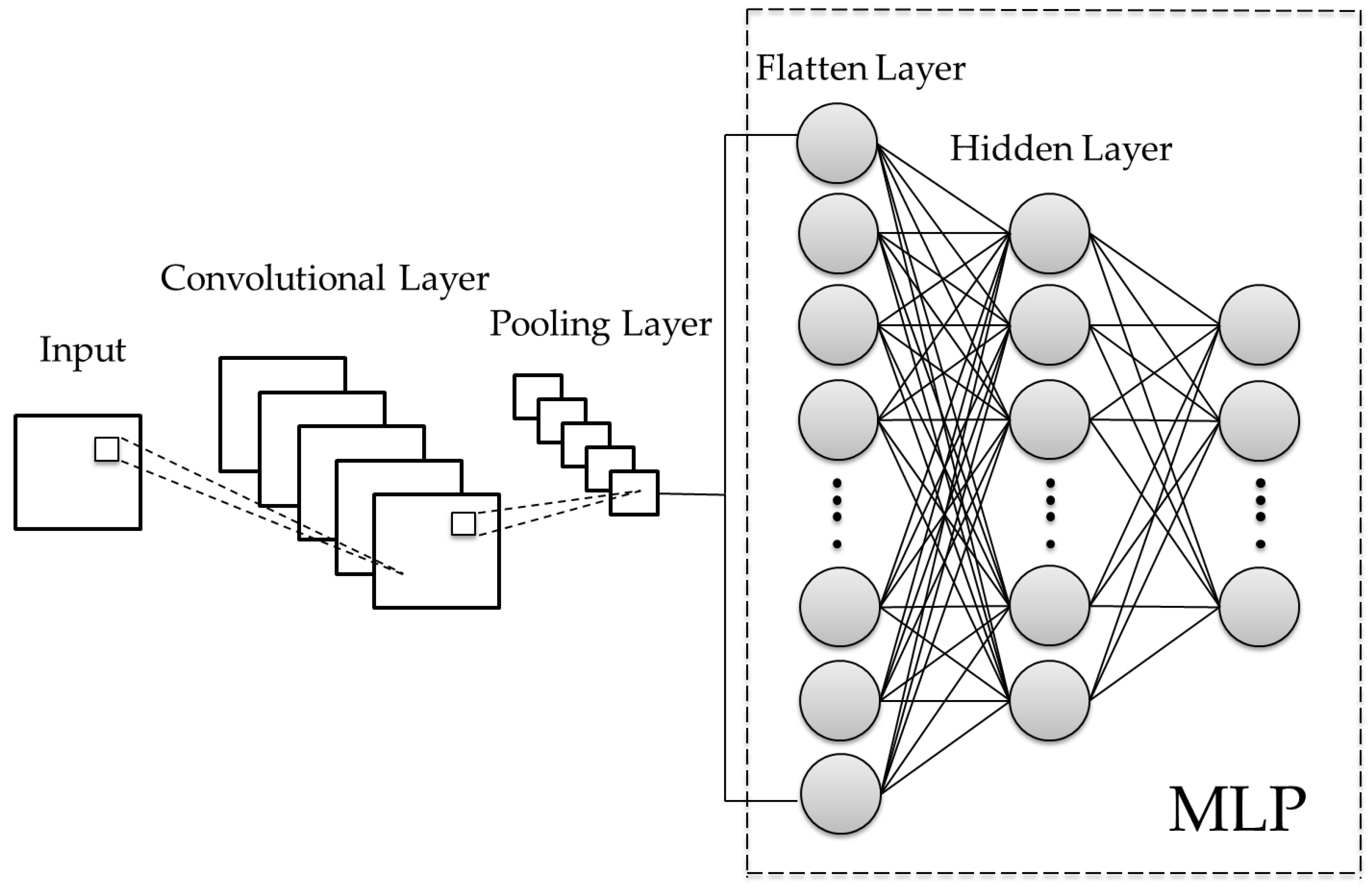
2. Brief of CNN
2.1. Convolutional Layer
2.2. Pooling Layer
2.3. Flatten Layer
2.4. Multilayer Perceptron
2.5. CNN Architecture of This Study
3. Experimental Study
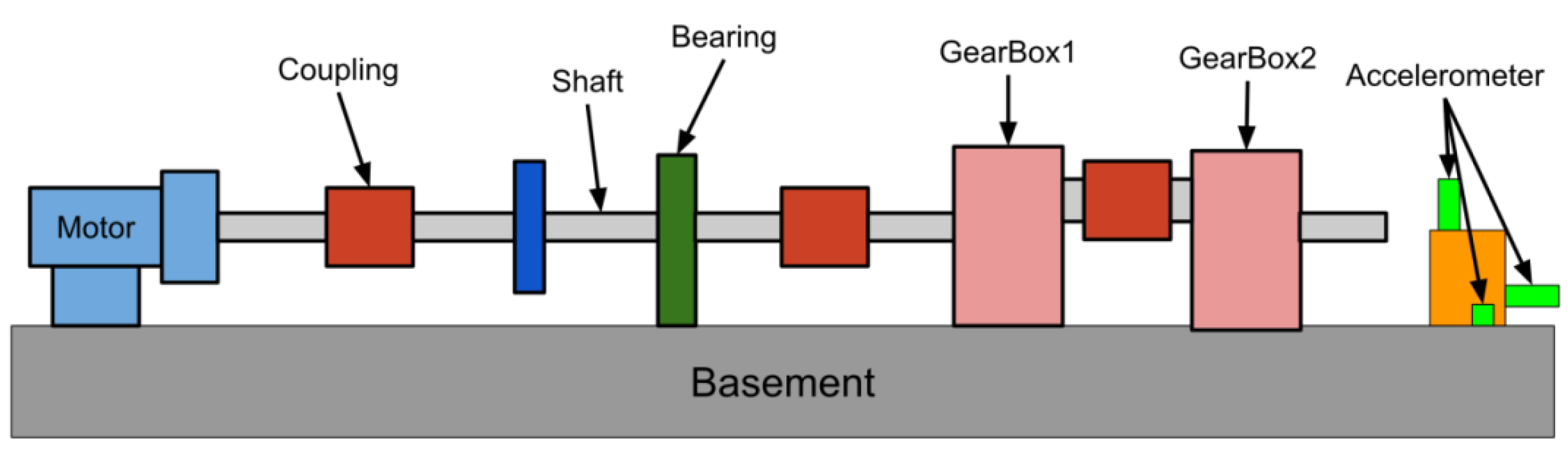
3.1. Description of Experimental System
- Wear: wear gear C and gear D by carborundum;
- Broken tooth: grind out one tooth of gear C;
- Loosening: no key is installed between gear and shaft, but they are tightly matched to make it possible to slip;
- Input shaft with misalignment: enlarge the input shaft bearing seat by 0.3 mm, and pad the input shaft so that it is not concentric with the shaft of gear A;
- Gear shaft with eccentricity: enlarge the bearing inner diameter of gear B and gear Cby 2 mm.
3.2. Remote Diagnosis
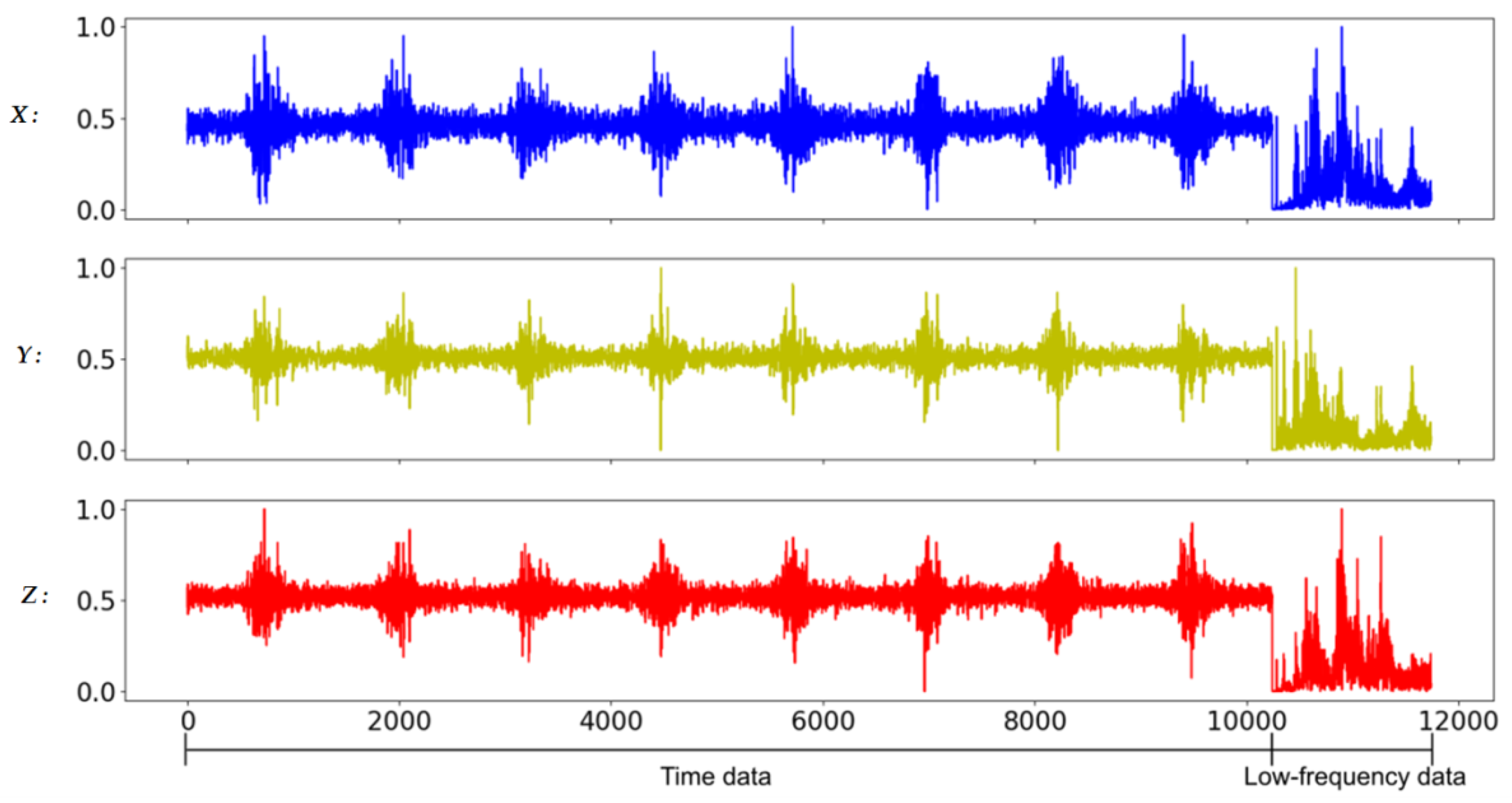
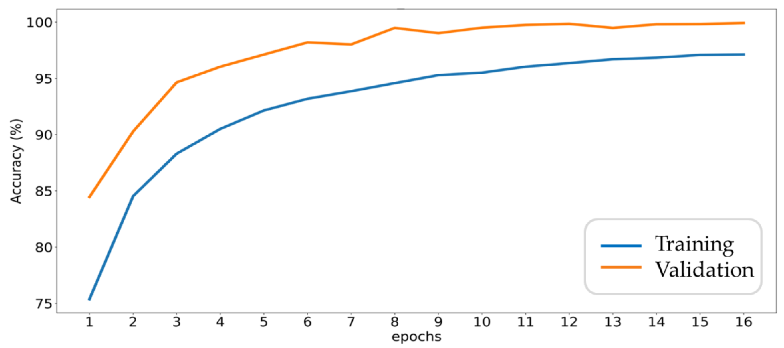
3.3. Experimental Results
3.3.1. Case (a): Comparison of Various Input Data Types and a Different Number of Neurons in a Fully Connected Layer
3.3.2. Case (b): Optimization of the Number of Convolution Kernels
4. Conclusions
Author Contributions
Funding
Conflicts of Interest
References
- Randall, R.B. A New Method of Modeling Gear Faults. J. Mech. Des. 1982, 104, 259–267. [Google Scholar] [CrossRef]
- Cortes, C.; Vapnik, V. Support-vector networks. Mach. Learn. 1995, 20, 273–297. [Google Scholar] [CrossRef]
- Kuriscak, E.; Marsalek, P.; Stroffek, J.; Toth, P.G. Biological context of Hebb learning in artificial neural networks, a review. Neurocomputing 2015, 152, 27–35. [Google Scholar] [CrossRef]
- Rumelhart, D.E.; Hinton, G.E.; Williams, R.J. Learning representations by back-propagating errors. Nature 1986, 323, 533–536. [Google Scholar] [CrossRef]
- LeCun, Y.; Bottou, L.; Bengio, Y.; Haffner, P. Gradient-based learning applied to document recognition. Proc. IEEE 1998, 86, 2278–2324. [Google Scholar] [CrossRef]
- Krizhevsky, A.; Sutskever, I.; Hinton, G.E. ImageNet Classification with Deep Convolutional Neural Networks. In Proceedings of the Advances in Neural Information Processing Systems (NIPS), Lake Tahoe, NV, USA, 3–6 December 2012; pp. 1097–1105. [Google Scholar]
- Zhang, L.; Han, Y.; Yang, Y.; Song, M.; Yan, S.; Tian, Q. Discovering Discriminative Graphlets for Aerial Image Categories Recognition. IEEE Trans. Image Process. 2013, 22, 5071–5084. [Google Scholar] [CrossRef] [PubMed]
- Song, J.; Gao, L.; Nie, F.; Shen, H.T.; Yan, Y.; Sebe, N. Optimized Graph Learning Using Partial Tags and Multiple Features for Image and Video Annotation. IEEE Trans. Image Process. 2016, 25, 4999–5011. [Google Scholar] [CrossRef] [PubMed]
- Tao, D.; Guo, Y.; Li, Y.; Gao, X. Tensor Rank Preserving Discriminant Analysis for Facial Recognition. IEEE Trans. Image Process. 2018, 27, 325–334. [Google Scholar] [CrossRef] [PubMed]
- Zhu, X.; Jing, X.-Y.; You, X.; Zuo, W.; Shan, S.; Zheng, W.-S. Image to Video Person Re-Identification by Learning Heterogeneous Dictionary Pair with Feature Projection Matrix. IEEE Trans. Inf. Forensics Secur. 2017, 13, 717–732. [Google Scholar] [CrossRef]
- Wang, X.; Gao, L.; Wang, P.; Sun, X.; Liu, X. Two-Stream 3-D convNet Fusion for Action Recognition in Videos with Arbitrary Size and Length. IEEE Trans. Multimed. 2018, 20, 634–644. [Google Scholar] [CrossRef]
- Wang, X.; Gao, L.; Song, J.; Zhen, X.; Sebe, N.; Shen, H.T. Deep appearance and motion learning for egocentric activity recognition. Neurocomputing 2018, 275, 438–447. [Google Scholar] [CrossRef]
- Chen, Z.; Li, C.; Sanchez, R.-V. Gearbox Fault Identification and Classification with Convolutional Neural Networks. Shock Vib. 2015, 2015. [Google Scholar] [CrossRef]
- Jia, F.; Lei, Y.; Lin, J.; Zhou, X.; Lu, N. Deep neural networks: A promising tool for fault characteristic mining and intelligent diagnosis of rotating machinery with massive data. Mech. Syst. Signal Process. 2016, 72–73, 303–315. [Google Scholar] [CrossRef]
- Janssens, O.; Slavkovikj, V.; Vervisch, B.; Stockman, K.; Loccufier, M.; Verstockt, S.; Van de Walle, R.; Van Hoecke, S. Convolutional Neural Network Based Fault Detection for Rotating Machinery. J. Sound Vib. 2016, 377, 331–345. [Google Scholar] [CrossRef]
- Jing, L.; Zhao, M.; Li, P.; Xu, X. A convolutional neural network based feature learning and fault diagnosis method for the condition monitoring of gearbox. Measurement 2017, 111, 1–10. [Google Scholar] [CrossRef]
- Zhang, W.; Peng, G.; Li, C.; Chen, Y.; Zhang, Z. A New Deep Learning Model for Fault Diagnosis with Good Anti-Noise and Domain Adaptation Ability on Raw Vibration Signals. Sensors 2017, 17, 425. [Google Scholar] [CrossRef] [PubMed]
- Zhao, M.; Kang, M.; Tang, B.; Pecht, M. Deep Residual Networks with Dynamically Weighted Wavelet Coefficients for Fault Diagnosis of Planetary Gearboxes. IEEE Trans. Ind. Electron. 2018, 65, 4290–4300. [Google Scholar] [CrossRef]
- Jiao, J.; Zhao, M.; Lin, J.; Zhao, J. A multivariate encoder information based convolutional neural network for intelligent fault diagnosis of planetary gearboxes. Knowl. Based Syst. 2018, 160, 237–250. [Google Scholar] [CrossRef]
- Wu, C.; Jiang, P.; Ding, C.; Feng, F.; Chen, T. Intelligent fault diagnosis of rotating machinery based on one-dimensional convolutional neural network. Comput. Ind. 2019, 108, 53–61. [Google Scholar] [CrossRef]
- Liang, P.; Deng, C.; Wu, J.; Yang, Z.; Zhu, J.; Zhang, Z. Compound Fault Diagnosis of Gearboxes via Multi-label Convolutional Neural Network and Wavelet Transform. Comput. Ind. 2019, 113, 103132. [Google Scholar] [CrossRef]
- Chen, Y.J. Hand-on Deep Learning by TensorFlow and Keras with Python, 1st ed.; FLAG: Taipei, Taiwan, 2019. (In Chinese) [Google Scholar]
- Zeiler, M.D.; Fergus, R. Visualizing and Understanding Convolutional Networks. In Proceedings of the 13th European Conference on Computer Vision (ECCV 2014), Zurich, Switzerland, 6–12 September 2014; pp. 818–833. [Google Scholar]
- Upton, E.; Halfacree, G. Raspberry Pi User Guide, 2nd ed.; John Wiley & Sons: Chichester, UK, 2014. [Google Scholar]


| No. Layer | Layer Type | Kernel Size (Stride) | Kernel Number | Output Size |
|---|---|---|---|---|
| 1 | Convolution | 5 × 1 (1) | 16 | 5116 × 16 |
| 2 | Max Pooling | 4 × 1 (4) | 16 | 1279 × 16 |
| 3 | Convolution | 51 × 1 (1) | 32 | 1229 × 32 |
| 4 | Max Pooling | 4 × 1 (4) | 32 | 307 × 32 |
| 5 | Dropout | 0.5 | / | 307 × 32 |
| 6 | Flatten | / | / | 9824 |
| 7 | Fully connected | 200 | / | 200 |
| 8 | Dropout | 0.5 | / | 200 |
| 9 | Output | 6 | / | 6 |
| Total parameters: | 2310345 | |||
| Training times | 10 |
| Epochs each time | 200 |
| Training/Test batch size | 50 |
| Training iteration per epoch | 441 |
| Test iteration per epoch | 189 |
| Number of Neurons | ||||||
|---|---|---|---|---|---|---|
| Input | 40 | 80 | 120 | 160 | 200 | 240 |
| FT (%) | 71.43 | 71.43 | 71.43 | 71.43 | 71.43 | 71.43 |
| LF (%) | 92.27 | 98.60 | 99.90 | 99.85 | 97.97 | 97.70 |
| FF (%) | 95.10 | 99.95 | 99.93 | 99.93 | 99.94 | 99.92 |
| FTCLF (%) | 71.43 | 95.28 | 98.25 | 99.60 | 98.96 | 71.43 |
| FTCFF (%) | 99.45 | 99.93 | 99.91 | 99.95 | 99.92 | 99.92 |
| Revised Model | Model before Revision | |
|---|---|---|
| Variable quantity | 75501 | 2385846 |
| Variable reduction | 2310345 | |
| Variable reduction (%) | 96.83 | |
| Number of Neurons | ||||||
|---|---|---|---|---|---|---|
| Input | 40 | 80 | 120 | 160 | 200 | 240 |
| FT (%) | 71.43 | 71.43 | 71.43 | 71.43 | 71.43 | 71.43 |
| LF (%) | 97.92 | 99.14 | 99.16 | 99.77 | 99.80 | 99.67 |
| FF (%) | 99.92 | 99.93 | 99.95 | 99.94 | 99.95 | 99.96 |
| FTCLF (%) | 86.81 | 97.88 | 97.93 | 99.07 | 99.39 | 99.37 |
| FTCFF (%) | 99.93 | 99.90 | 99.93 | 99.90 | 99.92 | 99.91 |
| Revised Model | Model before Revision | |
|---|---|---|
| Total training time (s) | 2160.05 | 2976.20 |
| Time reduction (s) | 816.15 | |
| Time reduction (%) | 27.42 | |
Publisher’s Note: MDPI stays neutral with regard to jurisdictional claims in published maps and institutional affiliations. |
© 2020 by the authors. Licensee MDPI, Basel, Switzerland. This article is an open access article distributed under the terms and conditions of the Creative Commons Attribution (CC BY) license (http://creativecommons.org/licenses/by/4.0/).
Share and Cite
Lin, M.-C.; Han, P.-Y.; Fan, Y.-H.; Li, C.-H.G. Development of Compound Fault Diagnosis System for Gearbox Based on Convolutional Neural Network. Sensors 2020, 20, 6169. https://doi.org/10.3390/s20216169
Lin M-C, Han P-Y, Fan Y-H, Li C-HG. Development of Compound Fault Diagnosis System for Gearbox Based on Convolutional Neural Network. Sensors. 2020; 20(21):6169. https://doi.org/10.3390/s20216169
Chicago/Turabian StyleLin, Ming-Chang, Po-Yu Han, Yi-Hua Fan, and Chih-Hung G. Li. 2020. "Development of Compound Fault Diagnosis System for Gearbox Based on Convolutional Neural Network" Sensors 20, no. 21: 6169. https://doi.org/10.3390/s20216169
APA StyleLin, M.-C., Han, P.-Y., Fan, Y.-H., & Li, C.-H. G. (2020). Development of Compound Fault Diagnosis System for Gearbox Based on Convolutional Neural Network. Sensors, 20(21), 6169. https://doi.org/10.3390/s20216169