Figure 1.
Structure of an Artificial Neural Network (ANN), which consists of multiple nonlinear transformations of the inputs .
Figure 1.
Structure of an Artificial Neural Network (ANN), which consists of multiple nonlinear transformations of the inputs .
Figure 2.
Predictions made by a Gaussian Process (GP). The data used to train the GP model are indicated with the black markers. The predictive distribution consists of a mean, indicated with the thick blue line, and a covariance of which the diagonal elements are used to calculate the confidence interval plotted around it. Since the prediction consists of a correlated Gaussian, it is possible to sample from this distribution, as shown in the plot. Every one of those samples possibly match with the real, underlying function.
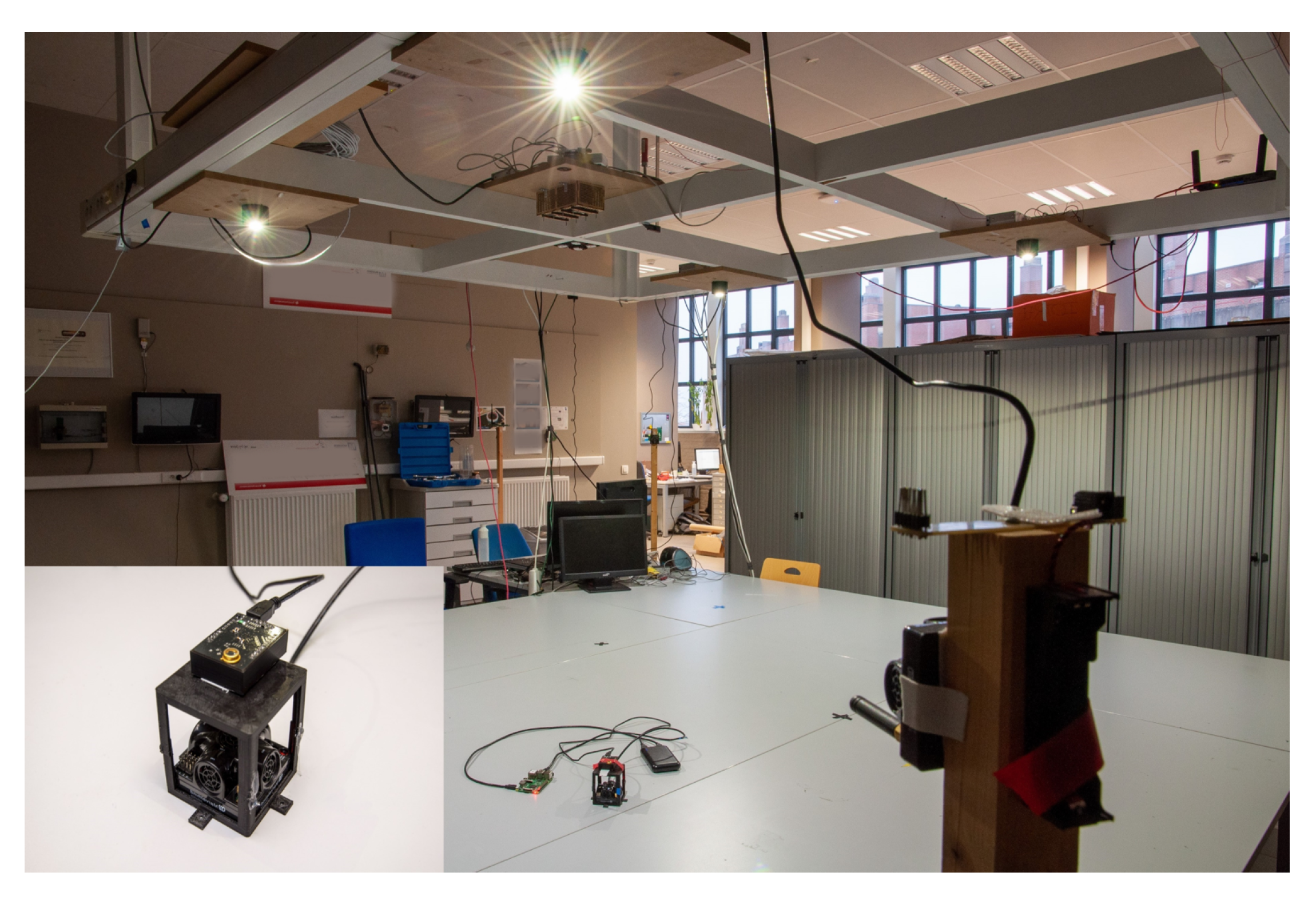
Figure 3.
A photo of the complete experimental set-up with four light-emitting diodes (LEDs) at height .
Figure 3.
A photo of the complete experimental set-up with four light-emitting diodes (LEDs) at height .
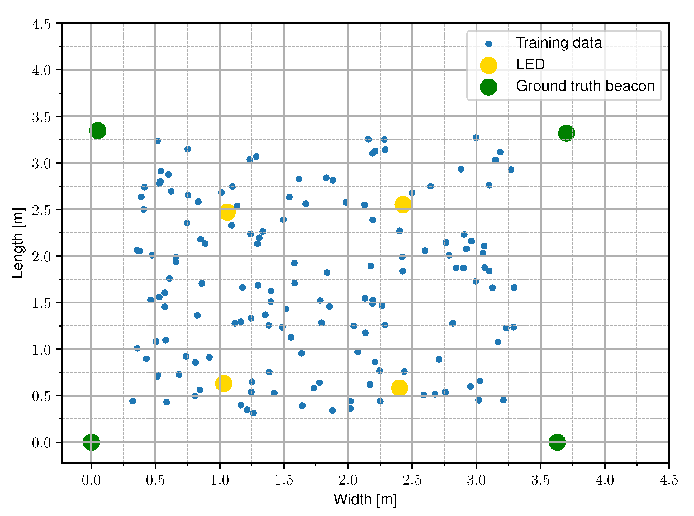
Figure 4.
A conceptual top view of the setup with four LEDs at a height h. The measured data from the experimental set-up is sampled randomly in the receiver plane.
Figure 4.
A conceptual top view of the setup with four LEDs at a height h. The measured data from the experimental set-up is sampled randomly in the receiver plane.
Figure 5.
A top view of the set-up with the angles of incidence at the photodiode (PD) highlighted for a single LED. The wide range of angles of incidence results in a representative experimental set-up.
Figure 5.
A top view of the set-up with the angles of incidence at the photodiode (PD) highlighted for a single LED. The wide range of angles of incidence results in a representative experimental set-up.
Figure 6.
Image of the custom designed receiver in the experimental setup, the device on the top is the Visible Light Positioning (VLP) receiver and the device on the bottom is the mobile node of the acoustic ground truth system (Marvelmind Robotics Super-NIA-3D).
Figure 6.
Image of the custom designed receiver in the experimental setup, the device on the top is the Visible Light Positioning (VLP) receiver and the device on the bottom is the mobile node of the acoustic ground truth system (Marvelmind Robotics Super-NIA-3D).
Figure 7.
A block schematic representation of the receiver circuit.
Figure 7.
A block schematic representation of the receiver circuit.
Figure 8.
A block schematic representation of the receiver on a system level.
Figure 8.
A block schematic representation of the receiver on a system level.
Figure 9.
Dust particles scattered on the aperture on the receiver, representing possible changes in the environment during operation of the VLP system where robustness is required.
Figure 9.
Dust particles scattered on the aperture on the receiver, representing possible changes in the environment during operation of the VLP system where robustness is required.
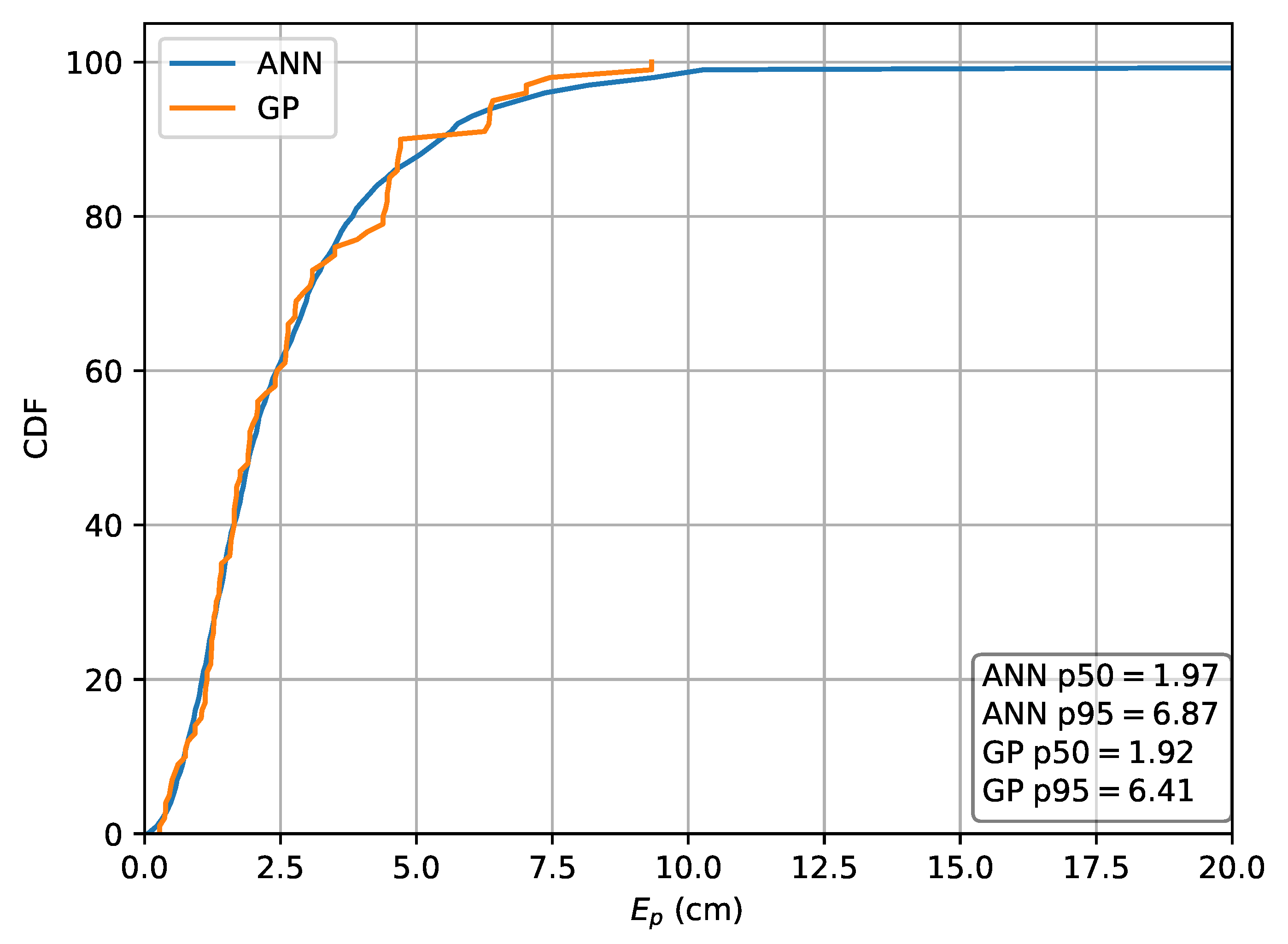
Figure 10.
Cumulative distribution of the error evaluated on set A for the Machine Learning (ML) methods in the case the absolute intensities r are used as features.
Figure 10.
Cumulative distribution of the error evaluated on set A for the Machine Learning (ML) methods in the case the absolute intensities r are used as features.
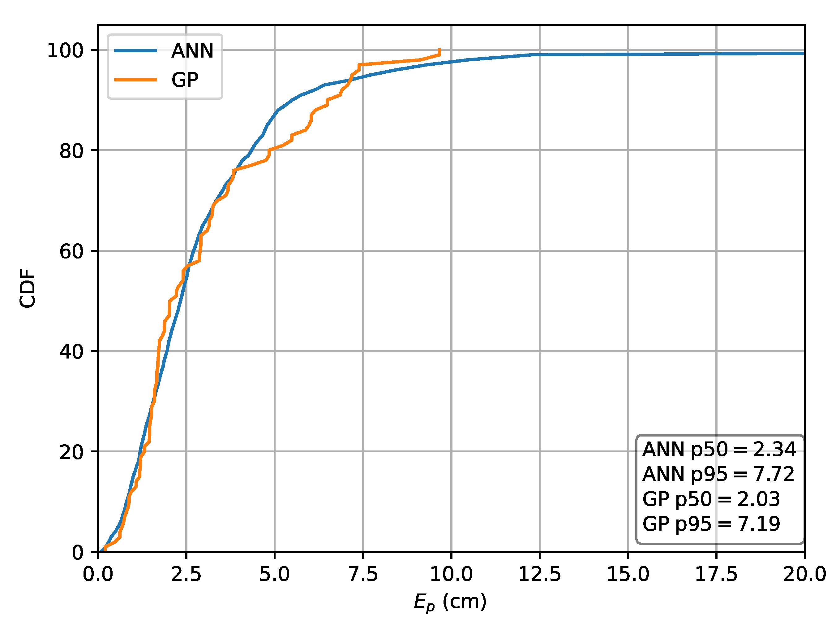
Figure 11.
Cumulative distribution of the error evaluated on set A for the ML methods in the case the relative intensities are used as features.
Figure 11.
Cumulative distribution of the error evaluated on set A for the ML methods in the case the relative intensities are used as features.
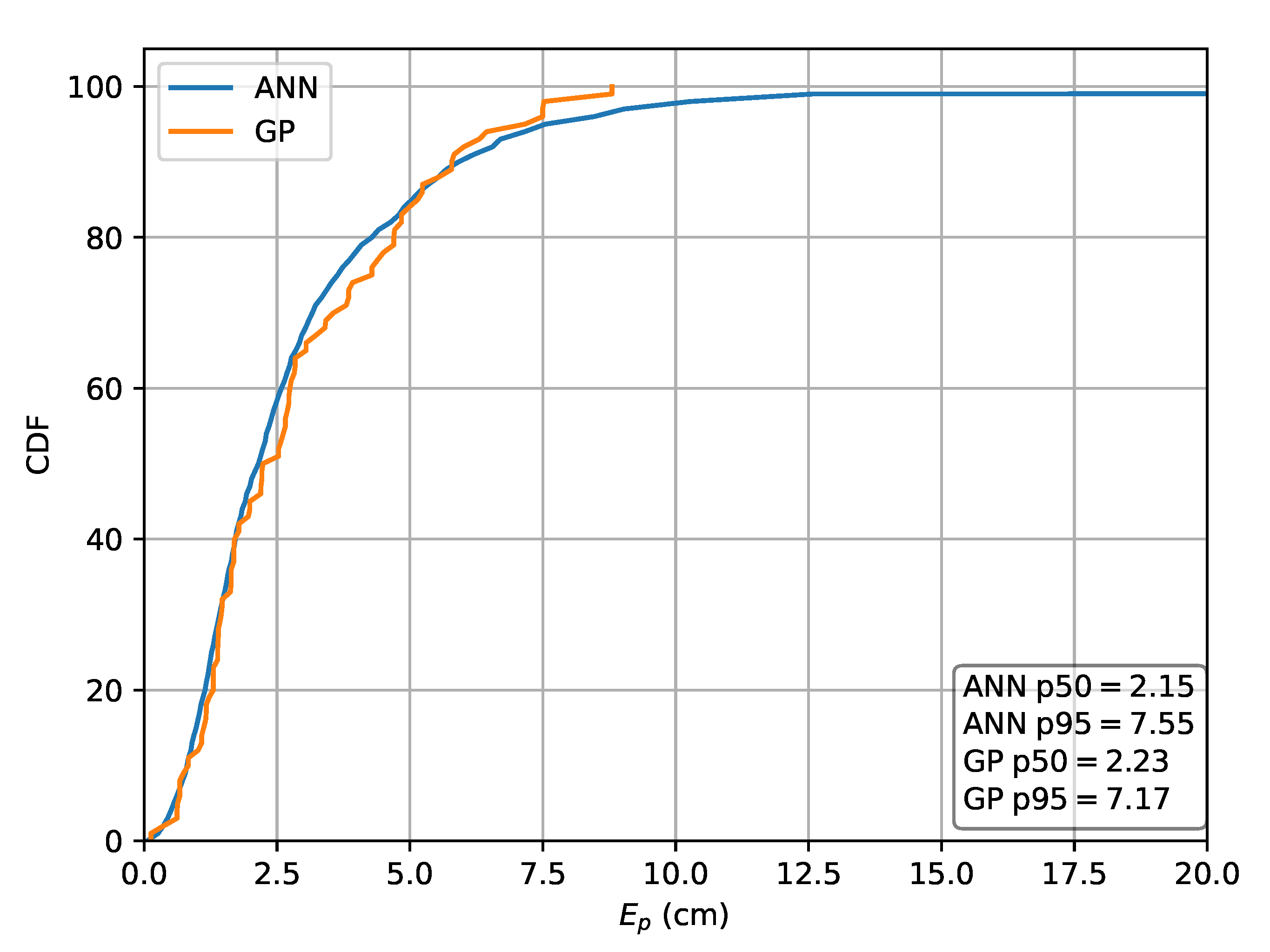
Figure 12.
Cumulative distribution of the error evaluated on set A for the ML methods in the case the relative intensities are used as features.
Figure 12.
Cumulative distribution of the error evaluated on set A for the ML methods in the case the relative intensities are used as features.
Figure 13.
Cumulative distribution of the error evaluated on set A for the absolute multilateration scheme using r as input.
Figure 13.
Cumulative distribution of the error evaluated on set A for the absolute multilateration scheme using r as input.
Figure 14.
Cumulative distribution of the error evaluated on set A for the relative multilateration schemes using and .
Figure 14.
Cumulative distribution of the error evaluated on set A for the relative multilateration schemes using and .
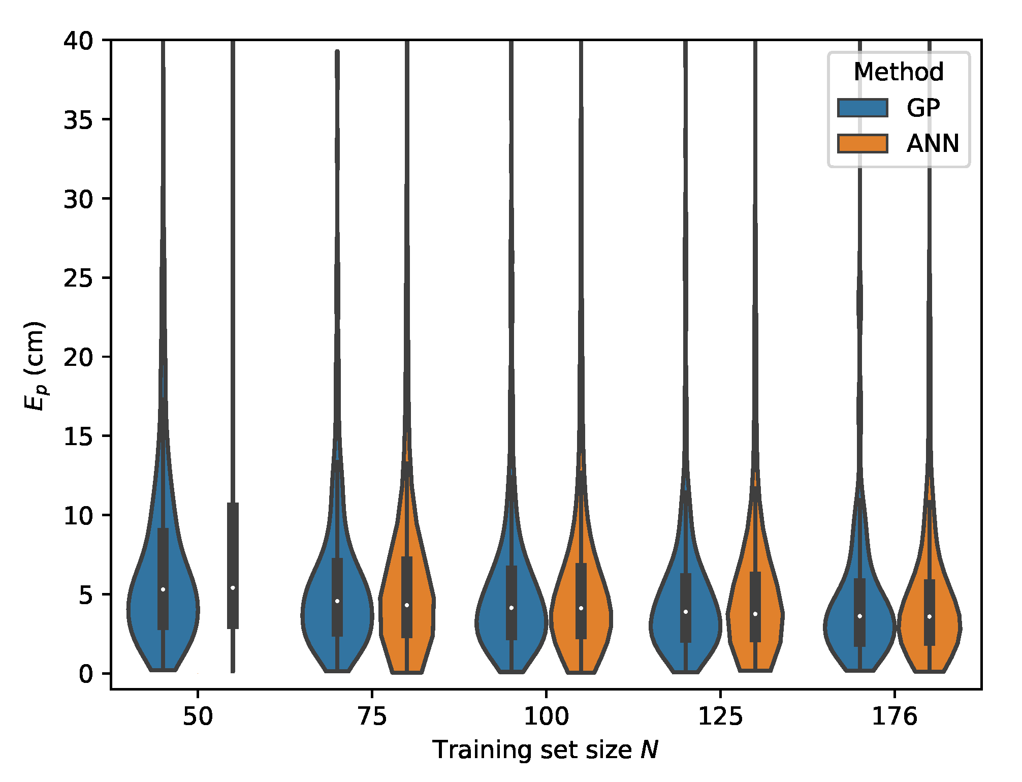
Figure 15.
Cross-validation with set C where the input features are used.
Figure 15.
Cross-validation with set C where the input features are used.
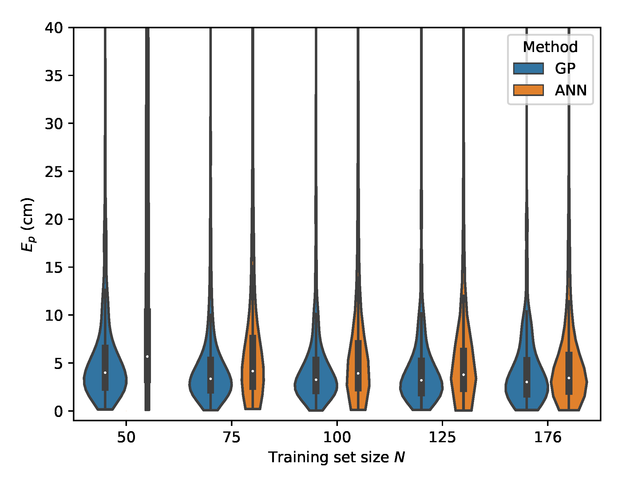
Figure 16.
Cross-validation with set B where the input features are used.
Figure 16.
Cross-validation with set B where the input features are used.
Figure 17.
Cross-validation with set D where the input features are used.
Figure 17.
Cross-validation with set D where the input features are used.
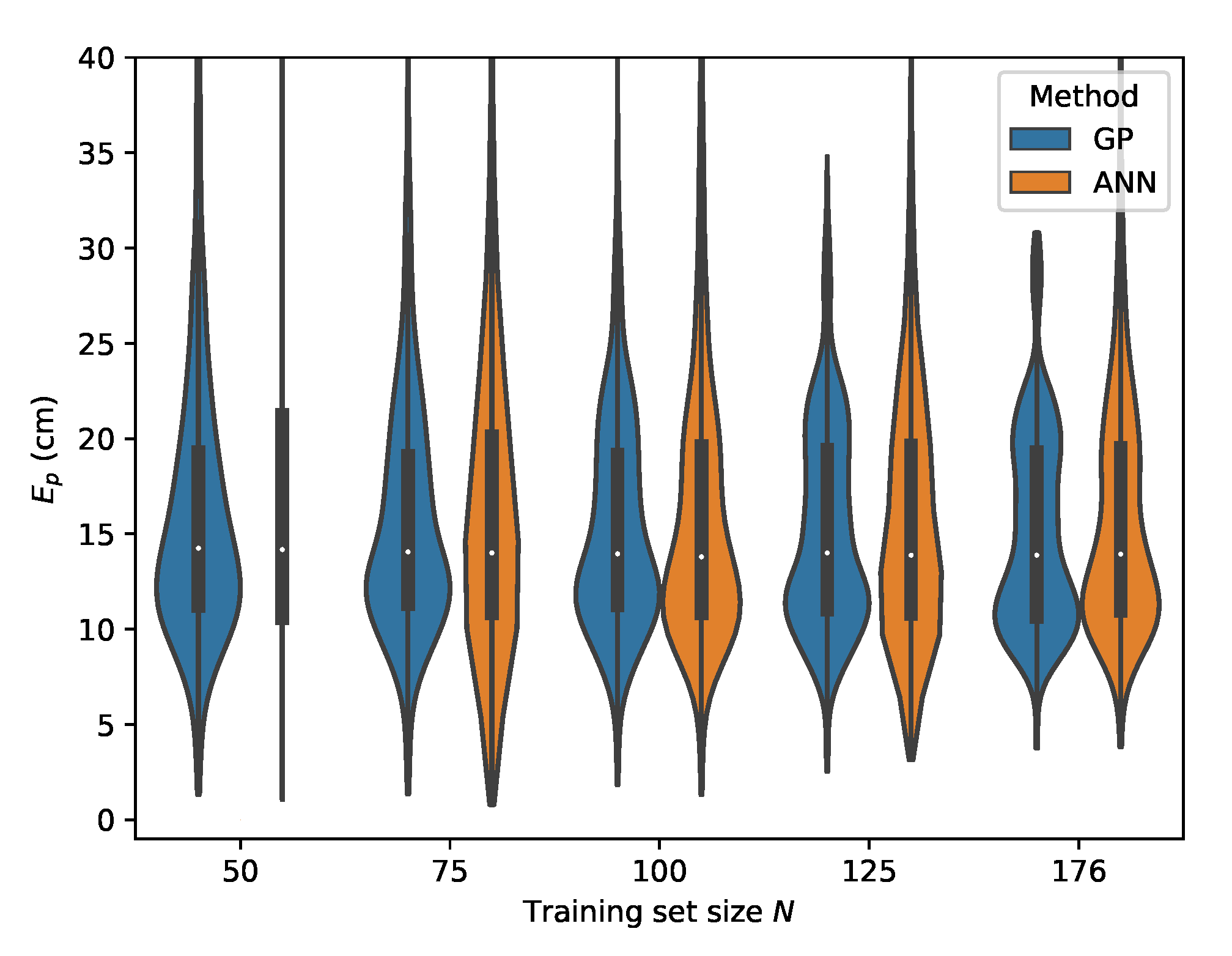
Figure 18.
Cross-validation with set E where the input features are used.
Figure 18.
Cross-validation with set E where the input features are used.
Figure 19.
Cross-validation with set C where the input features are used.
Figure 19.
Cross-validation with set C where the input features are used.
Figure 20.
Cross-validation with set B where the input features are used.
Figure 20.
Cross-validation with set B where the input features are used.
Figure 21.
Cross-validation with set D where the input features are used.
Figure 21.
Cross-validation with set D where the input features are used.
Figure 22.
Cross-validation with set E where the input features are used.
Figure 22.
Cross-validation with set E where the input features are used.
Table 1.
The system parameters of the experimental set-up.
Table 1.
The system parameters of the experimental set-up.
| System Parameters | Parameter Value |
|---|
| Room Dimensions | 3 × 3 |
| Height h | |
| Number of LEDs | 4 |
| LED Lambertian order m | 1 |
Table 2.
Parameters of the VLP receiver in the experimental set-up.
Table 2.
Parameters of the VLP receiver in the experimental set-up.
| Receiver Parameters | Parameter Value |
|---|
| Photodiode area size | 13 mm2 |
| TIA Gain | 40 k |
| DC-bias voltage | V |
| LPF cut off frequency | 36 kHz |
| Sampling frequency | 128 kHz |
| ADC-range | V |
| ADC precision | 14 bit |
Table 3.
Summary of the acquired datasets with their reference name and the context describing the experiment circumstances.
Table 3.
Summary of the acquired datasets with their reference name and the context describing the experiment circumstances.
| Dataset | Size | Context |
|---|
| A | 177 | Set measured with LED current of 350 mA. This dataset is used as training set for the ML methods. |
| B | 165 | Set measured with LED current of 300 mA. |
| C | 127 | Set measured with LED current of 250 mA. |
| D | 174 | Set measured with white chalk dust scattered on the PD surface, LED current 350 mA. |
| E | 162 | Set measured with sawdust scattered on the PD surface, on the PD surface, LED current 350 mA. |
Table 4.
The p50 and p95 errors expressed in () for the evaluated schemes on dataset A.
Table 4.
The p50 and p95 errors expressed in () for the evaluated schemes on dataset A.
| | Performance on Dataset A |
|---|
| | Input r | Input | Input |
|---|
| Configuration | p50 | p95 | p50 | p95 | p50 | p95 |
|---|
| MLP | 1.97 | 6.87 | 2.34 | 7.72 | 2.15 | 7.55 |
| GP | 1.92 | 6.41 | 2.03 | 7.19 | 2.23 | 7.17 |
| MLAT | 3.28 | 8.17 | 4.09 | 46.06 | 4.33 | 41.03 |
Table 5.
The p50 and p95 percentiles of the error expressed in () for the classical multilateration algorithm.
Table 5.
The p50 and p95 percentiles of the error expressed in () for the classical multilateration algorithm.
| Classical Multilateration Model Using the Absolute Intensities r as Features |
|---|
| Data | p50 | p95 |
|---|
| B | 10.36 | 27.30 |
| C | 25.82 | 54.86 |
| D | 16.42 | 35.38 |
| E | 32.68 | 58.47 |
Table 6.
The p50 and p95 percentiles of the error expressed in () for the Gaussian process model.
Table 6.
The p50 and p95 percentiles of the error expressed in () for the Gaussian process model.
| Gaussian Process Model Using |
|---|
| | | | | | |
| Data | p50 | p95 | p50 | p95 | p50 | p95 | p50 | p95 | p50 | p95 |
| B | 5.30 | 19.45 | 4.56 | 15.73 | 4.14 | 15.99 | 3.89 | 12.38 | 3.61 | 11.52 |
| C | 8.91 | 20.91 | 8.61 | 19.19 | 8.38 | 19.32 | 8.11 | 18.49 | 7.77 | 18.39 |
| D | 10.55 | 24.25 | 10.12 | 22.46 | 9.95 | 21.89 | 9.83 | 20.92 | 9.99 | 20.53 |
| E | 14.25 | 29.47 | 14.05 | 26.96 | 13.95 | 26.2 | 14.01 | 24.03 | 13.88 | 22.95 |
Table 7.
The p50 and p95 percentiles of the error expressed in () for the Multilayer Perceptron model.
Table 7.
The p50 and p95 percentiles of the error expressed in () for the Multilayer Perceptron model.
| Multi Layer Perceptron Model Using |
|---|
| | | | | | |
| Data | p50 | p95 | p50 | p95 | p50 | p95 | p50 | p95 | p50 | p95 |
| B | 5.41 | 39.62 | 4.31 | 19.68 | 4.12 | 18.69 | 3.75 | 15.98 | 3.59 | 15.23 |
| C | 8.77 | 27.26 | 8.25 | 21.78 | 8.11 | 20.86 | 7.69 | 19.68 | 7.98 | 18.72 |
| D | 10.65 | 32.65 | 10.22 | 22.15 | 9.88 | 22.12 | 9.83 | 22.12 | 9.76 | 20.33 |
| E | 14.18 | 55.07 | 14.00 | 30.26 | 13.79 | 30.95 | 13.88 | 27.39 | 13.93 | 27.74 |
Table 8.
The p50 and p95 percentiles of the error expressed in () for the Gaussian process model for the second relative RSS scheme.
Table 8.
The p50 and p95 percentiles of the error expressed in () for the Gaussian process model for the second relative RSS scheme.
| Gaussian Process Model Using |
|---|
| | | | | | |
| Data | p50 | p95 | p50 | p95 | p50 | p95 | p50 | p95 | p50 | p95 |
| B | 4.00 | 17.09 | 3.36 | 13.77 | 3.25 | 12.74 | 3.20 | 11.60 | 3.02 | 10.82 |
| C | 8.27 | 20.44 | 7.96 | 19.09 | 8.03 | 18.81 | 7.85 | 17.59 | 7.68 | 18.80 |
| D | 10.10 | 20.77 | 9.89 | 19.61 | 9.90 | 19.67 | 9.65 | 19.40 | 9.27 | 19.54 |
| E | 14.02 | 26.38 | 14.14 | 25.27 | 14.33 | 25.56 | 14.11 | 25.31 | 13.66 | 25.52 |
Table 9.
50 and 95 percentile of the error expressed in () for the Multilayer Perceptron model for the second relative RSS scheme.
Table 9.
50 and 95 percentile of the error expressed in () for the Multilayer Perceptron model for the second relative RSS scheme.
| Multi Layer Perceptron Model Using |
|---|
| | | | | | |
| Data | p50 | p95 | p50 | p95 | p50 | p95 | p50 | p95 | p50 | p95 |
| B | 5.43 | 40.57 | 4.30 | 30.25 | 3.70 | 21.92 | 3.53 | 16.43 | 3.49 | 15.48 |
| C | 8.59 | 45.16 | 7.88 | 25.37 | 7.67 | 22.29 | 7.76 | 19.23 | 7.65 | 20.58 |
| D | 10.80 | 39.6 | 9.95 | 27.13 | 9.73 | 21.21 | 9.68 | 19.77 | 9.52 | 19.81 |
| E | 14.05 | 54.54 | 13.62 | 40.59 | 13.99 | 32.97 | 13.78 | 27.93 | 13.82 | 27.55 |
Table 10.
The p50 and p95 percentiles of the error expressed in () for the relative multilateration schemes.
Table 10.
The p50 and p95 percentiles of the error expressed in () for the relative multilateration schemes.
| Multilateration Cross Validation |
|---|
| | Features | Features |
|---|
| Data | p50 | p95 | p50 | p95 |
|---|
| B | 4.10 | 112 | 4.49 | 125.67 |
| C | 6.56 | 35.77 | 6.74 | 47.47 |
| D | 8.83 | 62.79 | 9.16 | 62.98 |
| E | 13.39 | 82.48 | 13.19 | 57.15 |


