3.1. Activity-Aware GNSS Control
It is well known that the energy consumption of sensor-based mobile devices can be remarkably saved by introducing the adaptive sensor control strategy associated with domain-specific knowledge [
30,
31]. For example, Krause et al. [
32] investigated the trade-off of adaptive sensor control strategies between the human-motion classification performance and the sampling rate, which can be specialized to handle the support vector machine (SVM) and Markov chain model. Andersson et al. [
33] introduced the two step control method for activating the power-hungry sensors based on the sensing results of low-power but less-accurate sensors. Considering the movements of football players as described for the tracking test scenario in [
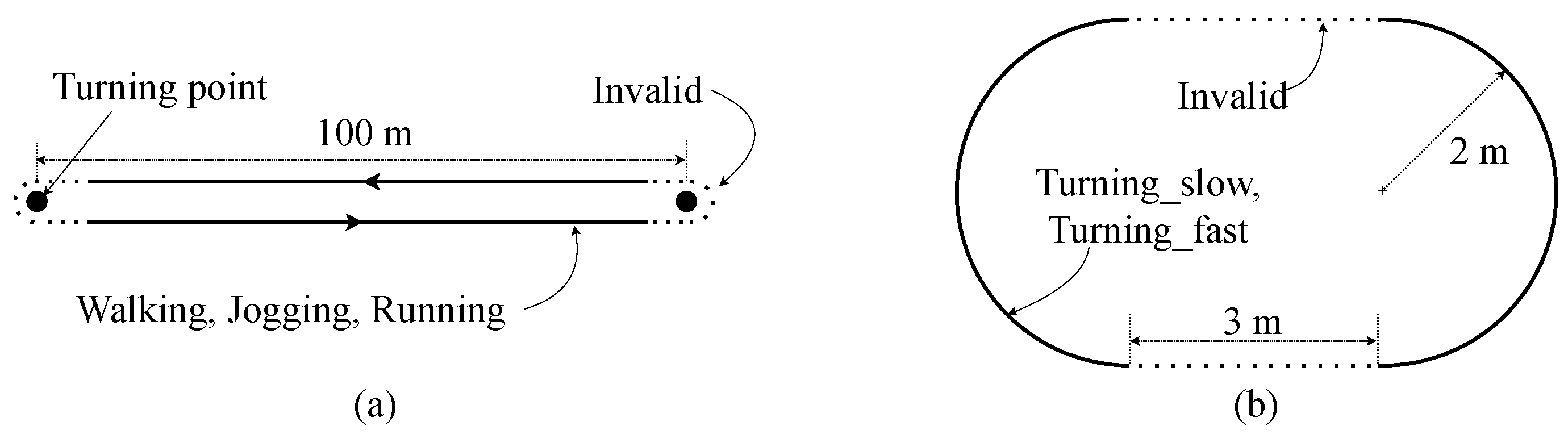
28], inspired by the prior works, we designed an advanced firmware-level optimization to reduce the activation frequency of the GNSS module depending on the athletic actions of players. By categorizing the movement types using the current sensing data, as conceptually illustrated in
Figure 5, more precisely, we can disable the GNSS receiver for a moment when the player stays from a certain position during the match time. For the case study, in this work, we define six activities that frequently occur at football matches, as summarized in
Table 2. To minimize the measurement errors caused by the reduced number of sensing samples, therefore, it is important to develop a simple but accurate algorithm on the embedded MCU for categorizing these pre-defined football activities.
For the straight-forward classification, similar to the prior work from [
34], we may directly use the speed measurements from the GNSS unit to set the intuitive thresholds to classify some human activities. For example, the athlete’s movement can be determined based on the fixed speed criteria defined in related papers [
29,
35], and then, the GNSS sampling rate for each activity can be adjusted to eliminate over-sampling data, as described in
Table 2. However, the speed value can only provide hints for categorizing the linear movements, and this approach cannot capture the rotation-related motions. Therefore, the energy-reduction from the straight-forward recognition is marginal due to the limited capability for categorizing the movement types of football players. In order to provide precise control of sensor modules, by using additional sensing signals from the IMU module, we develop the DCNN-based recognition of football activities, further reducing the energy consumption of the EPTS device.
3.2. Proposed DCNN-Based Classification of Football Activities
Recently, like the other classification issues [
36,
37,
38,
39], the algorithm-level performance of the human activity recognition (HAR) problem from IMU data has been remarkably improved by accepting DCNN approaches [
40,
41,
42,
43]. For example, the 1D CNN from [
44] utilizes the sensing data of a three axis accelerometer, finding the temporal features along each channel. Extending the dimension of the CNN architecture can capture the correlated features in multiple channel domains, improving the recognition accuracy of the HAR problem [
41]. Applying the pre-processing for multiple sensor measurements, furthermore, the quality of the CNN-based HAR system can be further improved as reported in [
42,
43]. For open-source datasets of motions in daily life [
40,
45,
46,
47],
Table 3 summarizes the performance of different CNN-based HAR systems in terms of the recognition accuracy, as well as the required memory size for storing the trained network. Note that the recent work from [
43] offers the smallest memory footprint among the existing works. Hence, we design a compact DCNN model based on the work from [
43], which is dedicated to recognizing the football activities at the resource-limited device.
Instead of using the open-source dataset directly [
40,
45,
46,
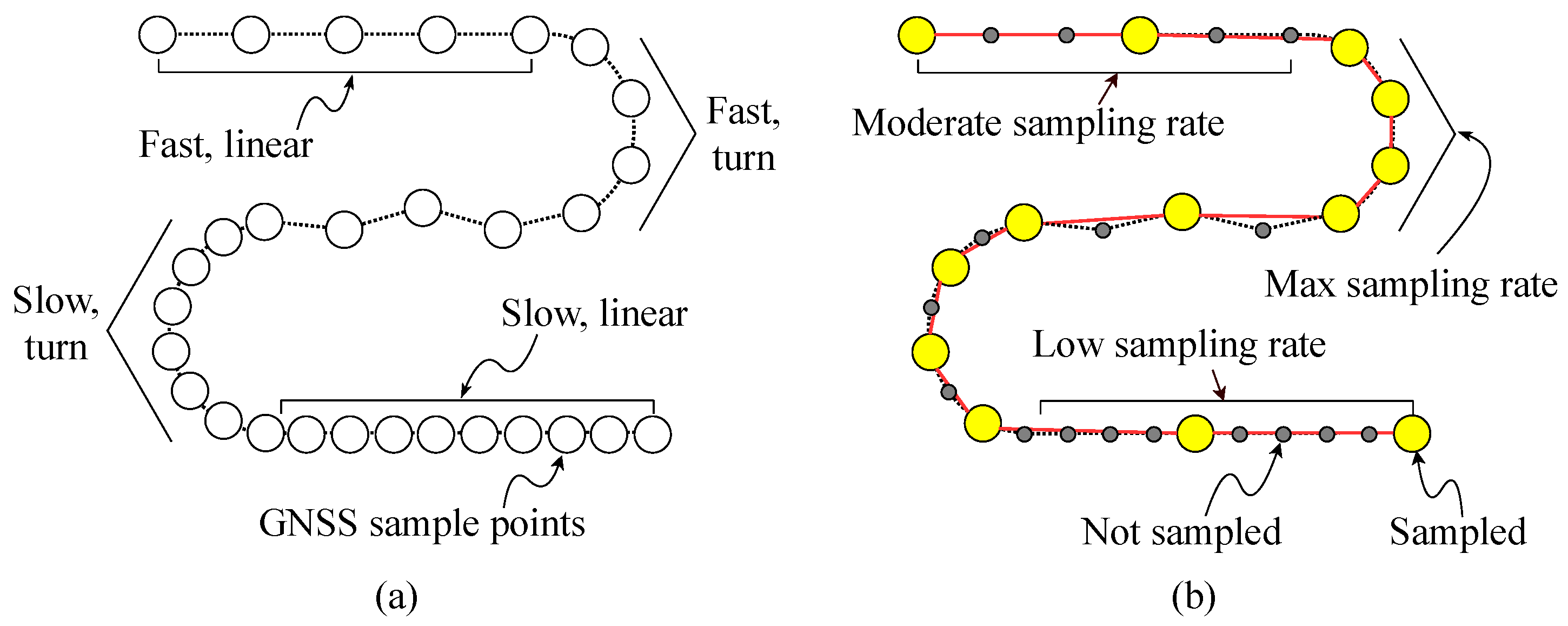
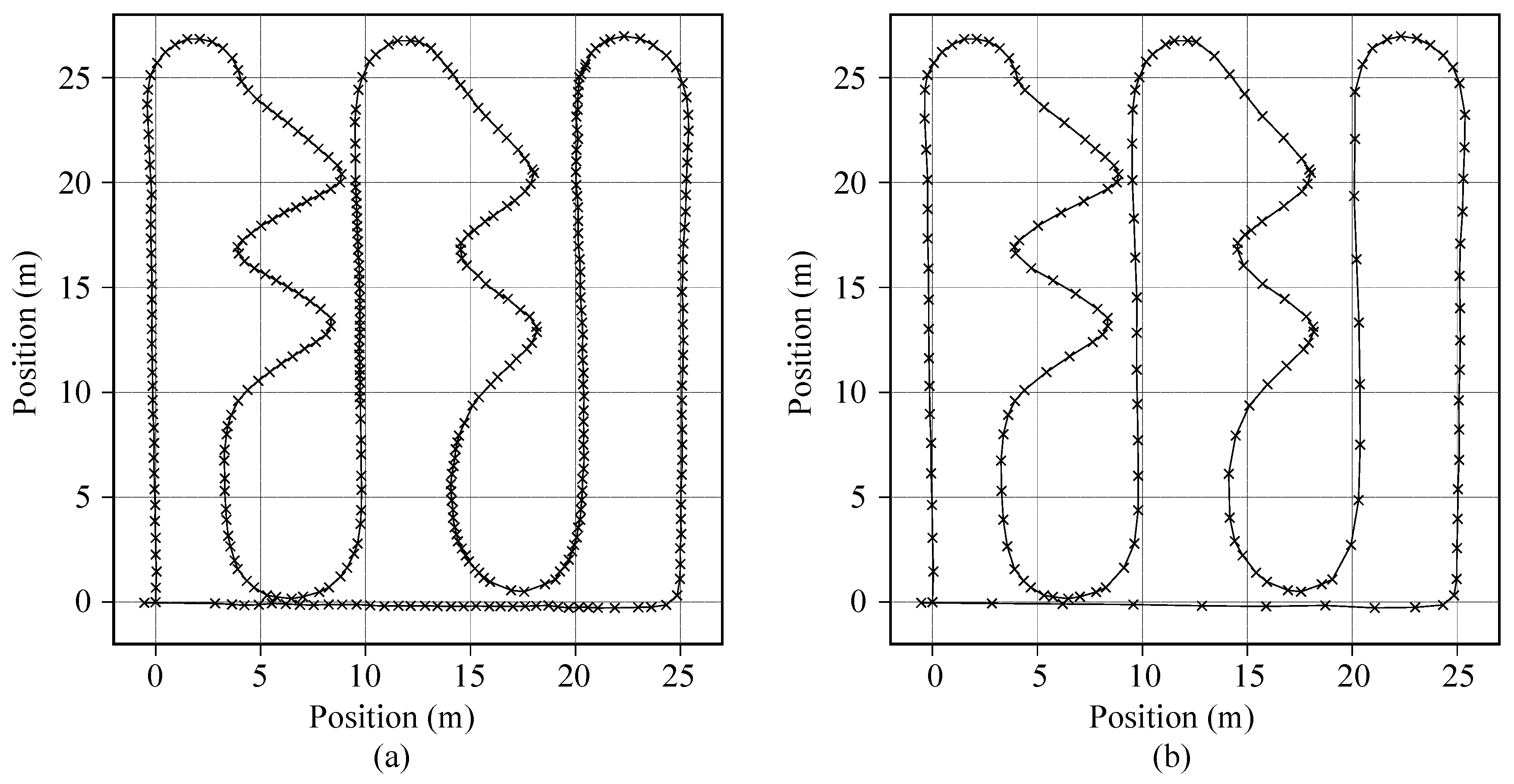
47], in order to generate a compact DCNN design, we collected actual data samples using the prototype EPTS devices. The custom dataset contains total 28,712 one second long samples of IMU measurements from five male subjects (age = 24.6 ± 2.2 years; height = 175.8 ± 3.7 cm; weight = 68.6 ± 3.6 kg). For the balanced data acquisition, in addition to using the standardized trajectory shown in
Figure 4a, we used two more tracks for collecting samples, which are more focused on the straight and rotation activities, as illustrated in
Figure 6a and
Figure 6b, respectively. Note that the acquired IMU samples were divided into training and testing sets by randomly selecting 400 samples from the collected dataset, as described in
Table 4.
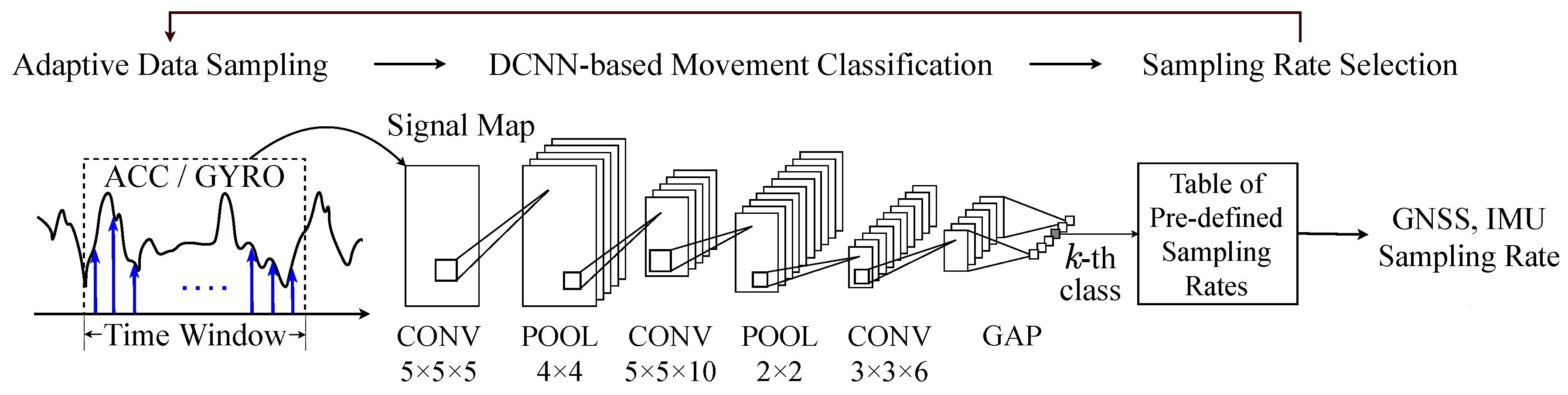
Figure 7 depicts the processing sequence of the proposed firmware-level EPTS sensor control that includes the low-cost CNN architecture for on-device processing. Similar to the prior work [
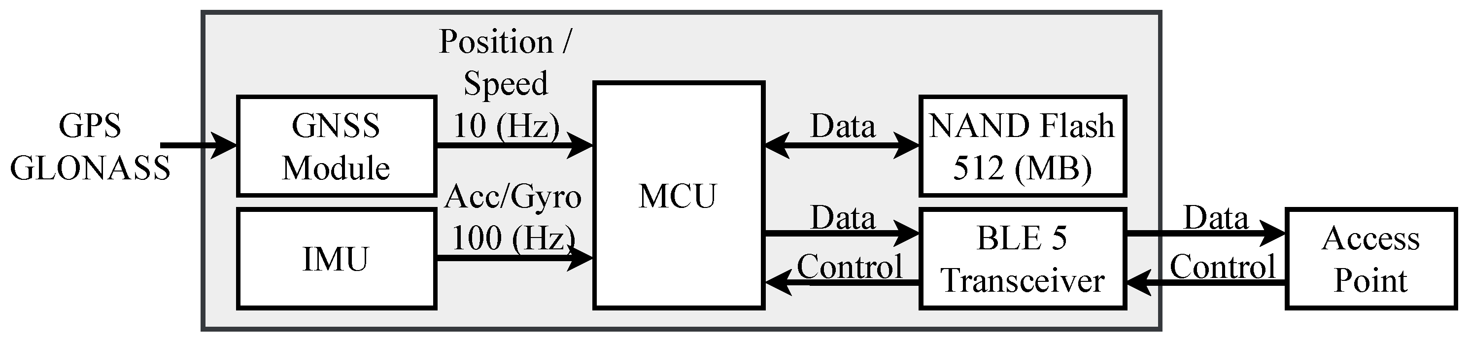
43], in every time window, we first gather measurement data from the multi-channel IMU sensor shown in
Figure 2 and then make a signal image by rearranging the sensor outputs in the 2D domain. More precisely, the signal image allows making all the sensor channels appear adjacent to each other. Then, as illustrated in
Figure 7, we deploy three convolution layers (CONVs) and two max pooling layers (POOLs) to find the temporal features for characterizing the target football activities. For the classifier, we simply introduce an global average pooling layer (GAP) rather than utilizing the computation-intensive fully-connected layers [
43], which can provide enough recognition accuracy to be used for categorizing the football activities. Targeting the football activity datasets from the real experimental environments, as a result, the baseline CNN architecture in this work achieves a recognition accuracy of 98.29% while requiring 7.56 KB for storing a whole network model based on 32 bit floating-point numbers.
To make the lightweight processing suitable for the on-device DCNN processing, the proposed DCNN architecture is further optimized by applying the quantization method [
48] to represent each network parameter with an 8 bit fixed-point number. In addition, the layer-fusing method from [
49] is utilized to merge two adjacent processing layers: one convolution layer and the following pooling layer, making a single processing layer associated with fewer parameters.
Table 5 compares the proposed DCNN architecture with the previous method from [
43], which provides the smallest model size among existing works, as summarized in
Table 3. For fair comparisons, we newly trained the prior work [
43] by using the custom dataset of football activities shown in
Table 4. Applying the post-training of 8 bit fixed-point parameters, note that we can remarkably compress the model size by 76.3% without degrading the algorithm-level performance. By only using the simple integer-based operations, note that the proposed quantized network even reduces the computing time for recognizing the football activities by 58.3% using the commercialized MCU module when compared to the previous state-of-the-art work using floating-point numbers. It is also possible to reduce the complexity of the prior design by exploiting the fixed-point number system. As depicted in
Table 5, however, the aggressive quantization severely degrades the algorithm-level performance of the DCNN model in [
43] as it necessitates intensive accumulations for realizing the fully-connected layer. Therefore, the proposed DCNN solution adopting cost-aware optimization schemes is a suitable option to recognize football activities at the resource-limited EPTS device.
3.3. DCNN-Based Sensing Rate Control for Energy-Optimized EPTS Operations
After categorizing the current football activity with the proposed lightweight DCNN architecture accepting the IMU measurements, it is possible to adjust the sampling frequency of the GNSS module for reducing the overall energy consumption of the EPTS device, which is the most energy-consuming component, as described in
Table 1. Due to the accurate classification results shown in
Table 5, it is easy to expect that the proposed activity-based control successfully maintains the amount of position errors with fewer GNSS samples when compared to the baseline EPTS operations shown in
Figure 4b. Compared to the straight-forward GNSS control that exploits the speed information only, the proposed technique obviously offers a better control option that further reduces the number of redundant GNSS samples, consequently relaxing the overheads to activate the power-hungry satellite accessing.
It is also possible to reduce the number of sensing operations on the IMU unit, which are used to make the signal image for CNN-based football activity recognition. Therefore, it is required to consider two sensing rates of the GNSS and IMU modules at the same time to find the optimal configuration in terms of energy consumption. For the sake of simplicity, we define
and
to denote the sampling rates of the GNSS and IMU units, respectively, which are used for developing the practical algorithm for developing the energy-optimized EPTS operations. Considering the allowable rates for each sensing device, the candidate set
S is defined by including the possible pairs of
and
, where
and
. For each football activity, we can find the optimal sensing-rate pair
, which can be obtained by solving the following problem:
Note that the cost function
is newly introduced as follows:
In the proposed cost function,
and
reflect the power consumption and the sensing error, respectively, where the hyper parameter
provides the scaling factor between two metrics. More specifically,
is simply calculated as:
where
and
denote the power consumption of the GNSS and IMU modules running at the given sampling rates, respectively. On the other hand, the second part of the cost function in Equation (
3), i.e.,
, can be formulated as follows:
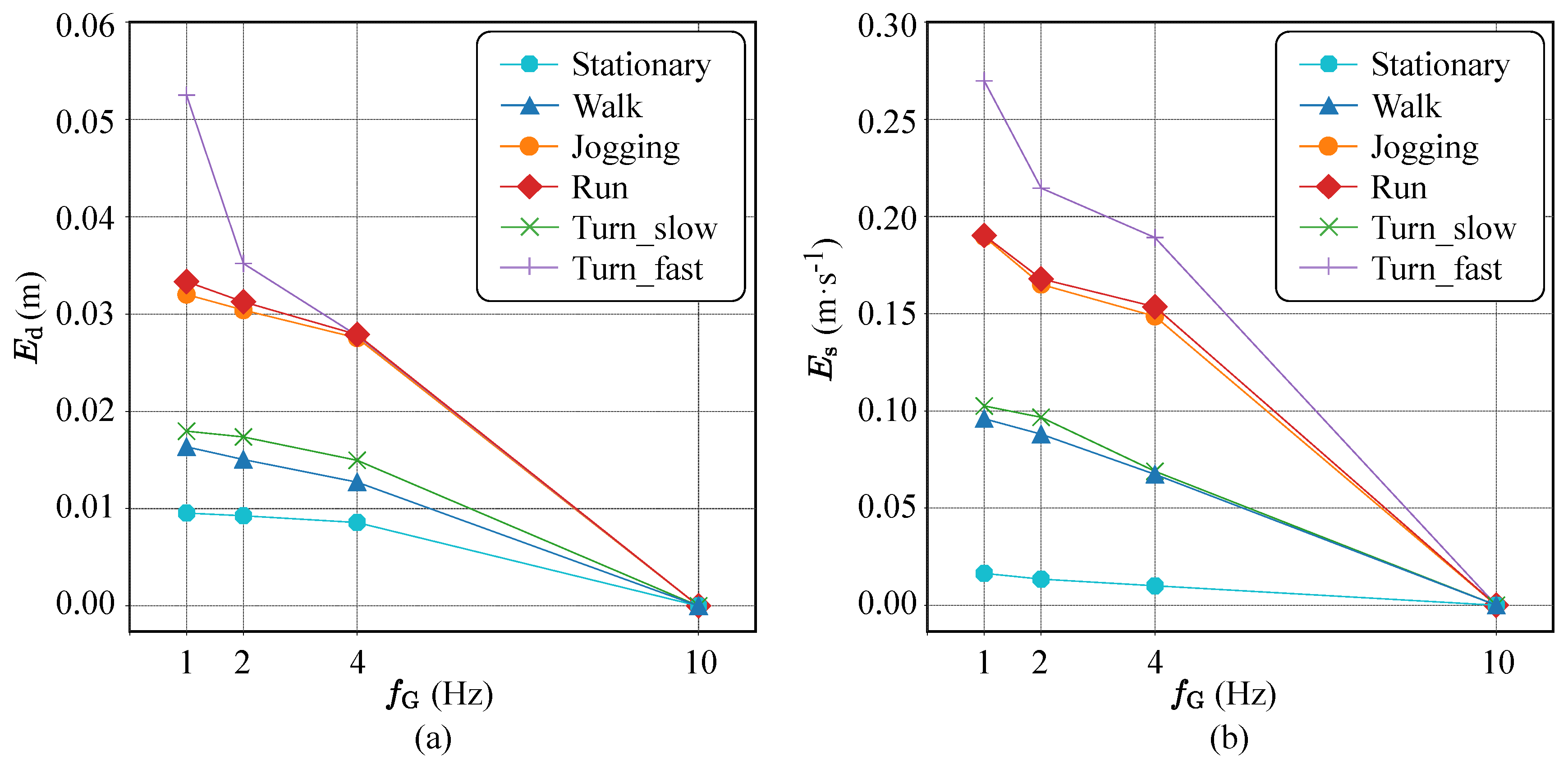
For the given configuration of the sampling rates, note that
and
are calculated by using Equation (
1), evaluating the errors in the distance and speed, respectively. We also define the second hyper parameter
that can adjust the ratio of the contributions between two errors.
Due to the impractical number of configurations defined by the candidate set
S, it is impractical to find the optimal set
by solving Equation (
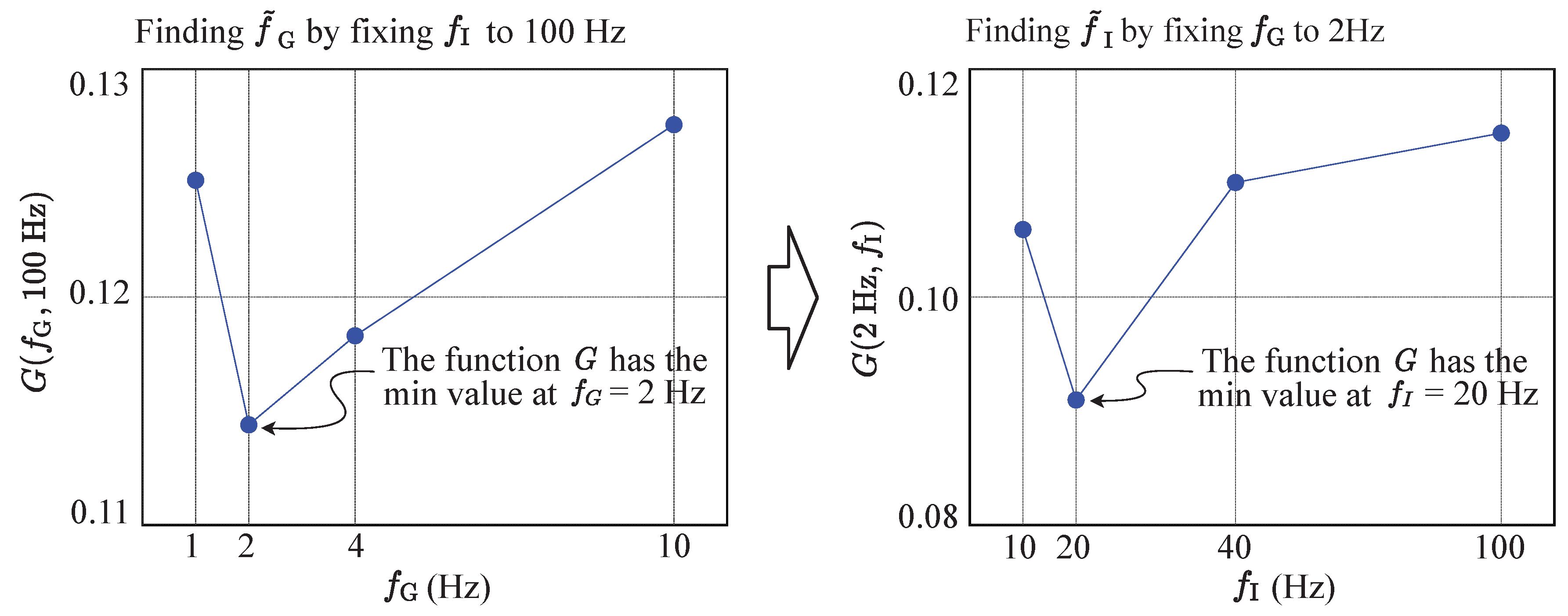
3) directly. For the practical solution, as described in Algorithm 1, we propose an iterative way to find a near-optimal configuration
, which still provides the energy-efficient, yet accurate EPTS operation. Starting from the initial configuration
, for each football activity described in
Table 2, we first reduce the sampling rate of the GNSS module, which minimizes the proposed cost function. Then, the IMU module is adjusted to find the better configuration. As described in Algorithm 1, this process is repeated until there is no change for the two sensing rates. Note that we always find the change of
first, as the energy consumption caused by the GNSS module is much larger that that of the IMU device, as reported in
Table 1. Without evaluating the complex cost function in the excessive number of times, as a result, we can simply get all the practical near-optimal configurations of sensing options for the target football activities, which is described in
Table 6. Compared to the threshold-based approach shown in
Table 2, which is a straight-forward way of using the speed information from the GNSS module directly, note that the proposed scheme provides a very aggressive control strategy with the high-quality DCNN-based activity classification, leading to the energy-optimized EPTS operations.
As we actively reduce the sensing rate of the IMU module, it is necessary to design an alternative way to construct the signal map, especially for the reduced number of IMU samples. In this work, we apply the linear interpolation to fill the IMU sensing data at the disabled time positions. By preserving the size of the input feature maps for different sensing rates, as a result, we can reuse the proposed DCNN architecture trained for the IMU sampling rate of 100 Hz, when the IMU module even goes to the power-saving mode measuring fewer samples. In other words, the proposed pre-processing always generates the same input format to the pre-designed network for the initial configuration of the sampling rates, i.e.,
, reducing the training overheads to consider the different configurations.
| Algorithm 1: Iterative method for finding the near-optimal sensing-rate configurations. |
 |


