Overview of Time Synchronization for IoT Deployments: Clock Discipline Algorithms and Protocols


Abstract
1. Introduction
- (i)
- transmitting a time report of a reference clock using a messaging protocol;
- (ii)
- mitigating non-determinism in message delivery and time measurements using a Clock Discipline Algorithm (CDA), and;
- (iii)
- adjusting the clocks.
2. Background
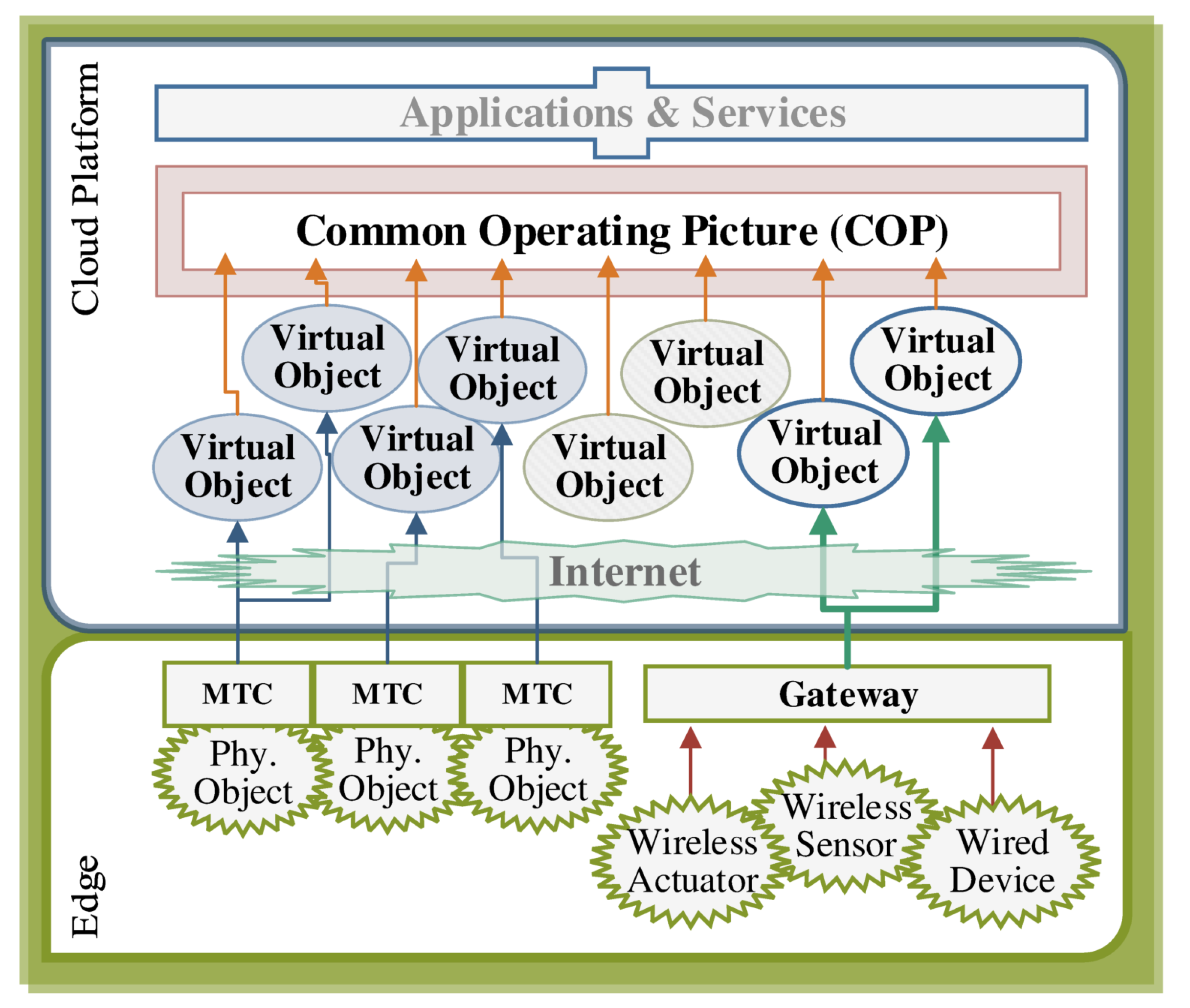
2.1. IoT Platform
- (i)
- Querying the universal time at which a specific event happened and observed by an object.
- (ii)
- Measuring the time difference between two events that are observed by different objects.
- (iii)
- Relatively ordering the events that are observed by different objects.
2.2. Motivation
2.3. Related Works
3. Clock Models
3.1. Software Clocks
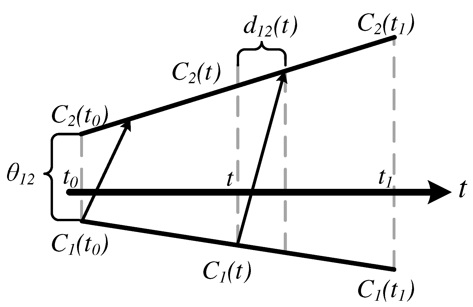
3.2. Clock Relation Model
3.2.1. Clocks on the Same Processor
3.2.2. Clocks on Different Processors
3.2.3. Numerical Example
3.3. Available Clock Relation Models
3.3.1. Offset-Only Model
3.3.2. Progressive Linear Model Only with Delivery Delay
3.3.3. Incremental Linear Model Only with Delivery Delays
3.3.4. High Order Models Only with Delivery Delay
3.3.5. Incremental Linear Model with Delivery Delay and Oscillator-Induced Correlation
3.3.6. Summary
4. Clock Discipline Algorithms
4.1. Background
| Algorithm 1 Calculate synchronized time |
|
4.1.1. Evaluation Metric
4.1.2. Evaluation Data
4.2. Offset-Only Estimation
4.3. Joint Batch Estimation of Offset and Skew
4.4. Adaptive Clock Skew Estimation
4.5. Clock Skew Estimation Using Incremental Linear Model with Delivery Delay and Oscillator-Induced Correlation
4.5.1. Batch Estimation
4.5.2. Recursive Estimation
4.5.3. Numerically Stable Recursive Estimation
4.6. Results and Discussion
4.6.1. Numerical Results
4.6.2. Discussion
| Algorithm 2 Batch clock parameter estimator |
|
| Algorithm 3 Recursive clock parameter estimator |
|
5. Time Synchronization Messaging
5.1. Background
5.1.1. Messaging Error Sources
- (i)
- send time,
- (ii)
- access time,
- (iii)
- propagation time, and
- (iv)
- receive time.
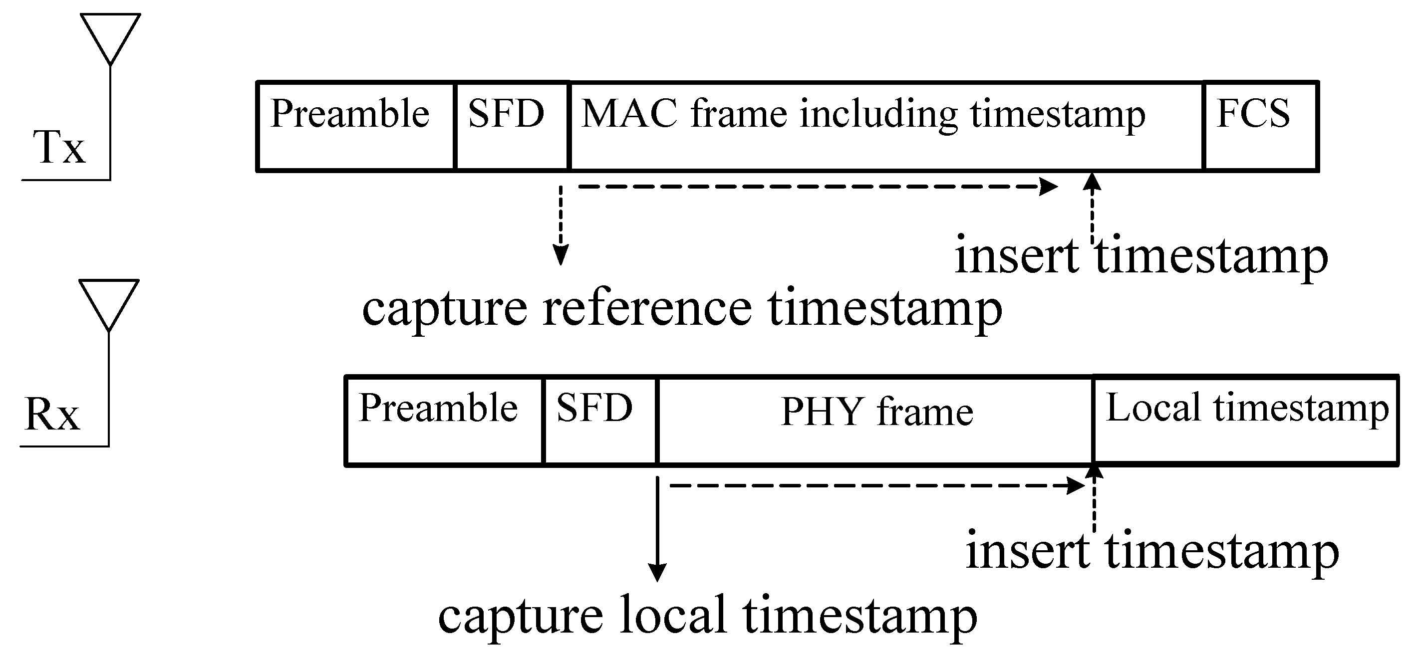
5.1.2. Timestamping
5.2. Messaging Schemes
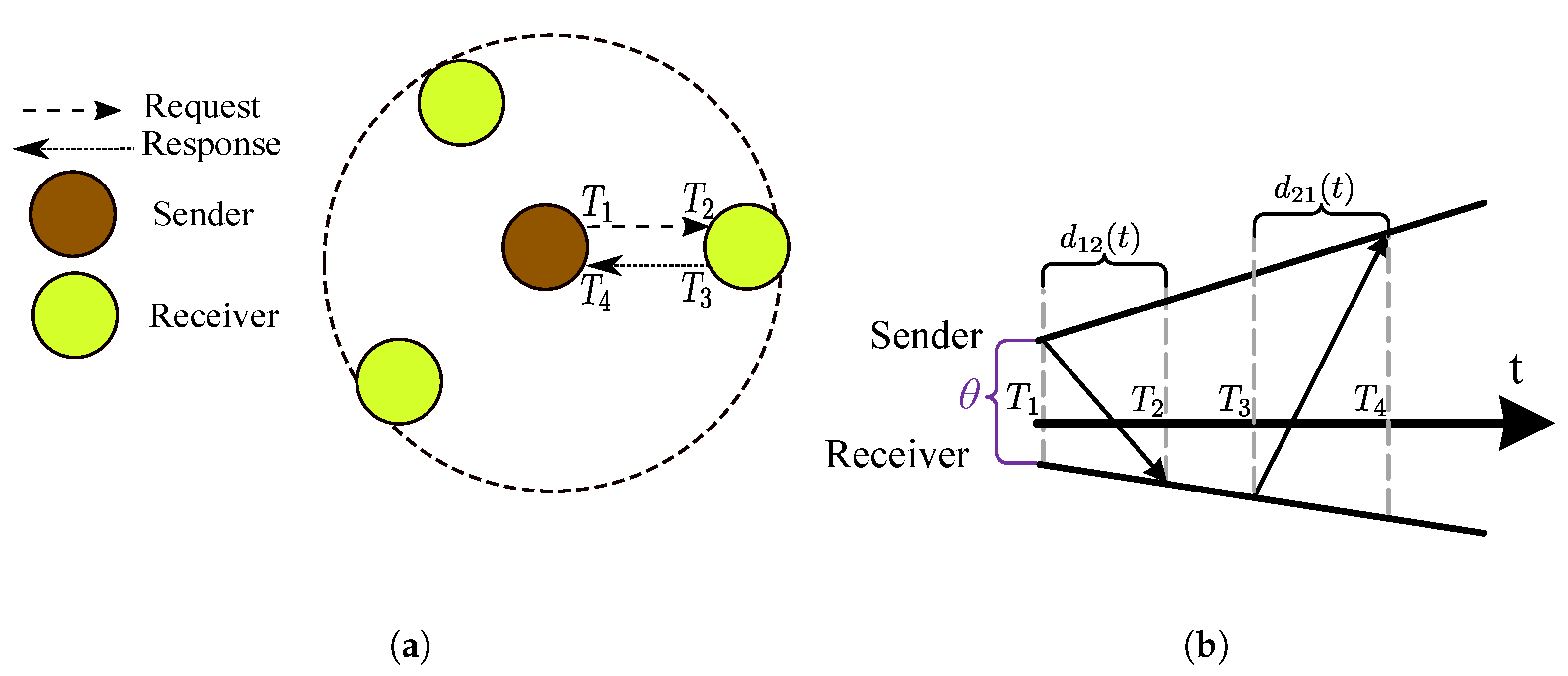
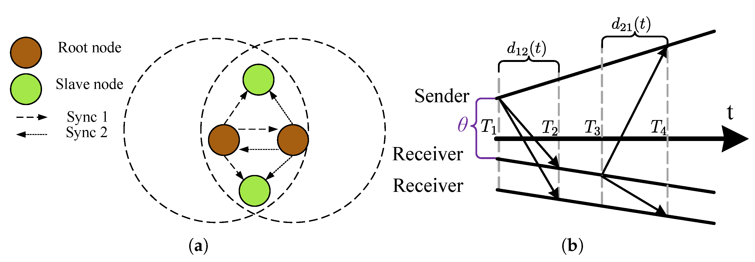
5.2.1. Two-Way Message Exchanges
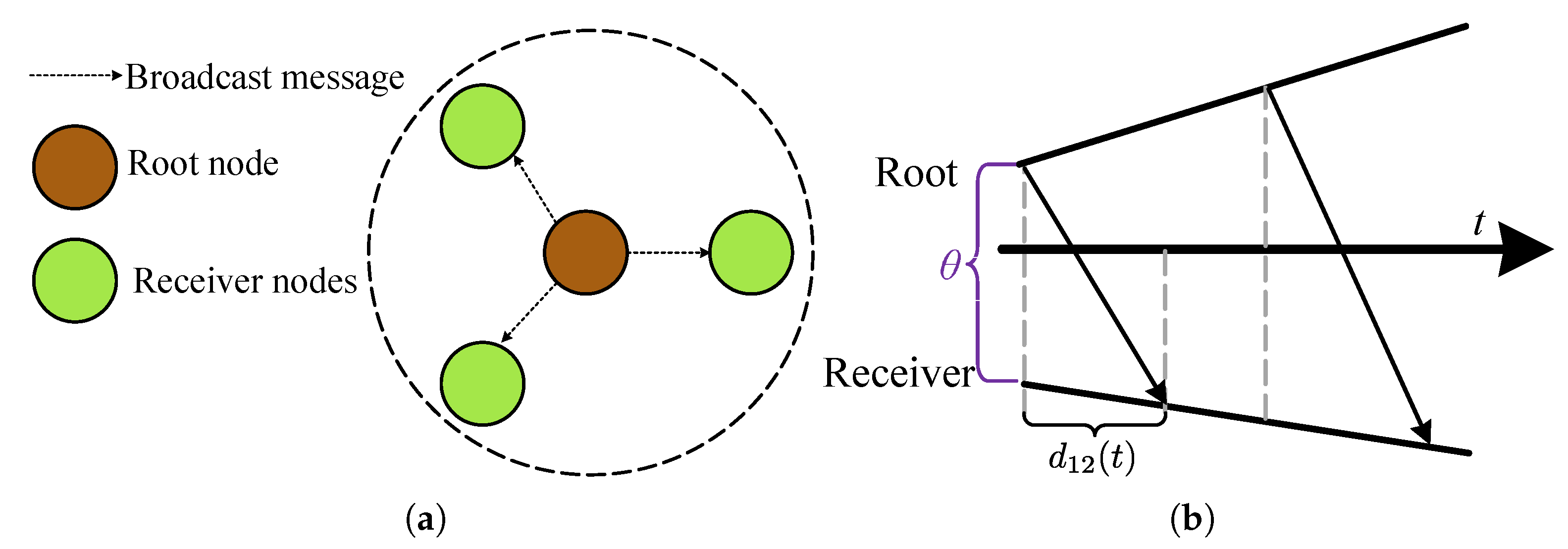
5.2.2. One-Way Message Dissemination
5.2.3. Receiver-only Synchronization
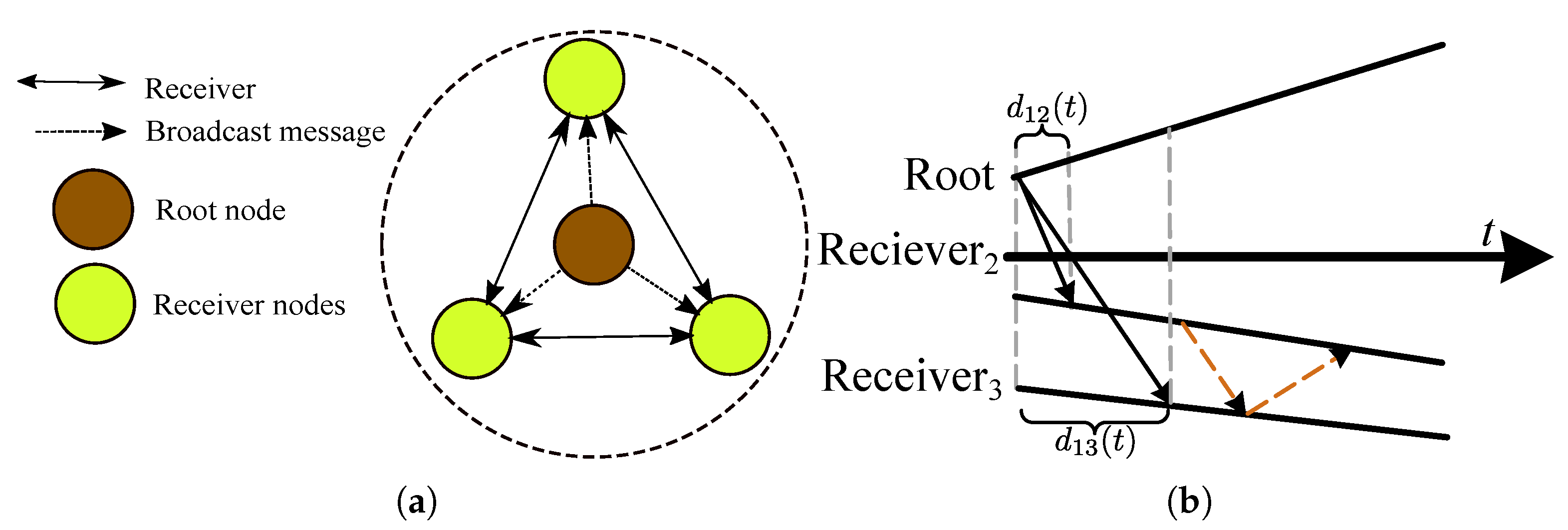
5.2.4. Receiver-receiver Synchronization
5.2.5. Discussion
5.3. Multi-hop Synchronization Schemes
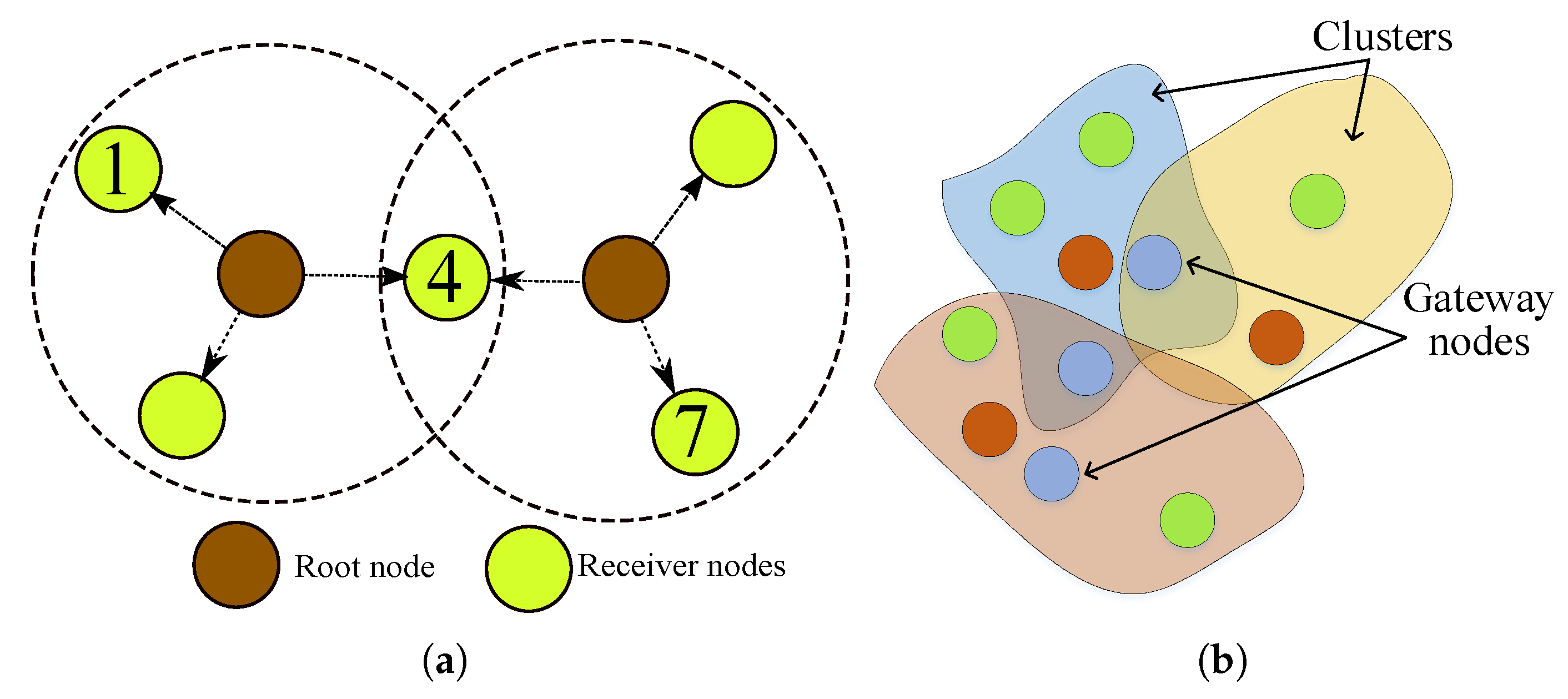
5.3.1. Cluster-Based Synchronization
5.3.2. Spanning-Tree Based Synchronization
5.3.3. Synchronous Diffusion
5.3.4. Distributed Synchronization
5.3.5. Discussion
5.4. Practical Problems
5.4.1. Synchronization Period
5.4.2. Reference Clock Source
5.4.3. Security
5.5. Time Synchronization in LAN and WAN
5.6. Summary
6. Examples
6.1. A Low-Power and Short-Range Network Synchronization
6.2. A Bluetooth-LE Star Network
7. Conclusions
Author Contributions
Funding
Acknowledgments
Conflicts of Interest
References
- CASAGRAS. Project Final Report: RFID and the Inclusive Model for the Internet of Things; Technical report European Union Framework 7 Project 216803; European Commission: London, UK, 2009. [Google Scholar]
- Moreno, M.F.; Cerqueira, R.; Colcher, S. Synchronization Abstractions and Separation of Concerns as Key Aspects to the Interoperability in IoT. In Interoperability, Safety and Security in IoT; Springer: Cham, Switzerland, 2016; pp. 26–32. [Google Scholar]
- Sachs, J.; Beijar, N.; Elmdahl, P.; Melen, J.; Militano, F.; Salmela, P. Capillary networks–a smart way to get things connected. Ericsson Rev. 2014, 8, 1–8. [Google Scholar]
- Zhu, Q.; Wang, R.; Chen, Q.; Liu, Y.; Qin, W. IoT gateway: Bridging wireless sensor networks into internet of things. In Proceedings of the 2010 IEEE/IFIP International Conference on Embedded and Ubiquitous Computing, Hong Kong, China, 11–13 December 2010; pp. 347–352. [Google Scholar]
- Akyildiz, I.F.; Su, W.; Sankarasubramaniam, Y.; Cayirci, E. Wireless sensor networks: A survey. Comput. Netw. 2002, 38, 393–422. [Google Scholar] [CrossRef]
- Gubbi, J.; Buyya, R.; Marusic, S.; Palaniswami, M. Internet of Things (IoT): A vision, architectural elements, and future directions. Future Gener. Comput. Syst. 2013, 29, 1645–1660. [Google Scholar] [CrossRef]
- Wu, Y.C.; Chaudhari, Q.; Serpedin, E. Clock synchronization of wireless sensor networks. IEEE Signal Process. Mag. 2011, 28, 124–138. [Google Scholar] [CrossRef]
- Savaglio, C.; Pace, P.; Aloi, G.; Liotta, A.; Fortino, G. Lightweight reinforcement learning for energy efficient communications in wireless sensor networks. IEEE Access 2019, 7, 29355–29364. [Google Scholar] [CrossRef]
- Allan, D.W. Time and frequency(time-domain) characterization, estimation, and prediction of precision clocks and oscillators. IEEE Trans. Ultrason. Ferroelectr. Freq. Control 1987, 34, 647–654. [Google Scholar] [CrossRef] [PubMed]
- Mills, D.L. Internet time synchronization: The network time protocol. IEEE Trans. Commun. 1991, 39, 1482–1493. [Google Scholar] [CrossRef]
- Mills, D. RFC 1305; IETF. 1992. Available online: https://tools.ietf.org/html/rfc1305 (accessed on 16 October 2020).
- Mills, D. RFC 4330; IETF. 2006. Available online: https://tools.ietf.org/html/rfc4330 (accessed on 16 October 2020).
- IEEE Std 1588-2008. IEEE Standard for a Precision Clock Synchronization Protocol for Networked Measurement and Control Systems (Revision of IEEE Std 1588-2002); IEEE: Piscataway, NJ, USA, 2008. [Google Scholar] [CrossRef]
- Gavras, A.; Karila, A.; Fdida, S.; May, M.; Potts, M. Future Internet Research and Experimentation: The FIRE Initiative. SIGCOMM Comput. Commun. Rev. 2007, 37, 89–92. [Google Scholar] [CrossRef]
- Miorandi, D.; Sicari, S.; De Pellegrini, F.; Chlamtac, I. Internet of things: Vision, applications and research challenges. Ad Hoc Netw. 2012, 10, 1497–1516. [Google Scholar] [CrossRef]
- Buckley, J. From RFID to the Internet of things. In Pervasive Networked Systems Conference Organised by DG Information Society and Media, Networks and Communication Technologies Directorate; CCAB: Brussels, Belgium, 2006. [Google Scholar]
- Lyytinen, K.; Yoo, Y. Ubiquitous computing. Commun. ACM 2002, 45, 63–96. [Google Scholar]
- Atzori, L.; Iera, A.; Morabito, G. The internet of things: A survey. Comput. Netw. 2010, 54, 2787–2805. [Google Scholar] [CrossRef]
- Sundararaman, B.; Buy, U.; Kshemkalyani, A.D. Clock synchronization for wireless sensor networks: A survey. Ad Hoc Netw. 2005, 3, 281–323. [Google Scholar] [CrossRef]
- Wald, L. Some terms of reference in data fusion. IEEE Trans. Geosci. Remote. Sens. 1999, 37, 1190–1193. [Google Scholar] [CrossRef]
- Bocca, M.; Eriksson, L.M.; Mahmood, A.; Jäntti, R.; Kullaa, J. A synchronized wireless sensor network for experimental modal analysis in structural health monitoring. Comput.-Aided Civ. Infrastruct. Eng. 2011, 26, 483–499. [Google Scholar] [CrossRef]
- Noel, A.B.; Abdaoui, A.; Elfouly, T.; Ahmed, M.H.; Badawy, A.; Shehata, M.S. Structural health monitoring using wireless sensor networks: A comprehensive survey. IEEE Commun. Surv. Tutor. 2017, 19, 1403–1423. [Google Scholar] [CrossRef]
- Gungor, V.; Hancke, G. Industrial Wireless Sensor Networks: Challenges, Design Principles, and Technical Approaches. IEEE Trans. Ind. Electron. 2009, 56, 4258–4265. [Google Scholar] [CrossRef]
- Raza, M.; Aslam, N.; Le-Minh, H.; Hussain, S.; Cao, Y.; Khan, N.M. A Critical Analysis of Research Potential, Challenges, and Future Directives in Industrial Wireless Sensor Networks. IEEE Commun. Surv. Tutor. 2018, 20, 39–95. [Google Scholar] [CrossRef]
- Petersen, S.; Carlsen, S. WirelessHART versus ISA100. 11a: The format war hits the factory floor. IEEE Ind. Electron. Mag. 2011, 5, 23–34. [Google Scholar] [CrossRef]
- Pister, K.; Doherty, L. TSMP: Time synchronized mesh protocol. In Proceedings of the IASTED Distributed Sensor Networks, Orlando, FL, USA, 16–18 November 2008; pp. 391–398. [Google Scholar]
- Watteyne, T.; Weiss, J.; Doherty, L.; Simon, J. Industrial IEEE802. 15.4e networks: Performance and trade-offs. In Proceedings of the 2015 IEEE International Conference on Communications (ICC), London, UK, 8–12 June 2015; pp. 604–609. [Google Scholar]
- IEEE Std 802.15.4-2015. IEEE Standard for Low-Rate Wireless Networks (Revision of IEEE Std 802.15.4-2011); IEEE: Piscataway, NJ, USA, 2016. [Google Scholar] [CrossRef]
- Vilajosana, X.; Watteyne, T.; Vučinić, M.; Chang, T.; Pister, K.S.J. 6TiSCH: Industrial Performance for IPv6 Internet-of-Things Networks. Proc. IEEE 2019, 107, 1153–1165. [Google Scholar] [CrossRef]
- Eze, E.C.; Zhang, S.; Liu, E. Vehicular ad hoc networks (VANETs): Current state, challenges, potentials and way forward. In Proceedings of the 20th International Conference on Automation and Computing, Cranfield, UK, 12–13 September 2014; pp. 176–181. [Google Scholar]
- Hasan, K.F.; Wang, C.; Feng, Y.; Tian, Y.C. Time synchronization in vehicular ad-hoc networks: A survey on theory and practice. Veh. Commun. 2018, 14, 39–51. [Google Scholar] [CrossRef]
- Hasan, K.F.; Feng, Y.; Tian, Y. GNSS Time Synchronization in Vehicular Ad-Hoc Networks: Benefits and Feasibility. IEEE Trans. Intell. Transp. Syst. 2018, 19, 3915–3924. [Google Scholar] [CrossRef]
- IEEE Std 802.11-2012. IEEE Standard for Information Technology–Telecommunications and Information Exchange between Systems Local and Metropolitan Area Networks–Specific Requirements Part 11: Wireless LAN Medium Access Control (MAC) and Physical Layer (PHY) Specifications (Revision of IEEE Std 802.11-2007); IEEE: Piscataway, NJ, USA, 2012. [Google Scholar] [CrossRef]
- IEEE Std 802.11p-2010. Standard for Information Technology– Local and Metropolitan Area Networks—Specific Requirements—Part 11: Wireless LAN Medium Access Control (MAC) and Physical Layer (PHY) Specifications Amendment 6: Wireless Access in Vehicular Environments (Amendment to IEEE Std 802.11-2007 as Amended by IEEE Std 802.11k-2008, IEEE Std 802.11r-2008, IEEE Std 802.11y-2008, IEEE Std 802.11n-2009, and IEEE Std 802.11w-2009); IEEE: Piscataway, NJ, USA, 2010. [Google Scholar] [CrossRef]
- Yan, Y.; Qian, Y.; Sharif, H.; Tipper, D. A Survey on Smart Grid Communication Infrastructures: Motivations, Requirements and Challenges. IEEE Commun. Surv. Tutor. 2013, 15, 5–20. [Google Scholar] [CrossRef]
- Lévesque, M.; Tipper, D. A survey of clock synchronization over packet-switched networks. IEEE Commun. Surv. Tutor. 2016, 18, 2926–2947. [Google Scholar] [CrossRef]
- Qiu, T.; Zhang, Y.; Qiao, D.; Zhang, X.; Wymore, M.L.; Sangaiah, A.K. A Robust Time Synchronization Scheme for Industrial Internet of Things. IEEE Trans. Ind. Inform. 2017. [Google Scholar] [CrossRef]
- Sivrikaya, F.; Yener, B. Time synchronization in sensor networks: A survey. IEEE Netw. 2004, 18, 45–50. [Google Scholar] [CrossRef]
- Ranganathan, P.; Nygard, K. Time synchronization in wireless sensor networks: A survey. Int. J. Ubicomp 2010, 1, 92–102. [Google Scholar] [CrossRef]
- Dalwadi, N.; Padole, M. An Insight into Time Synchronization Algorithms in IoT. In Data, Engineering and Applications; Springer: Singapore, 2019; pp. 285–296. [Google Scholar]
- Faizulkhakov, Y.R. Time synchronization methods for wireless sensor networks: A survey. Program. Comput. Softw. 2007, 33, 214–226. [Google Scholar] [CrossRef]
- Swain, A.R.; Hansdah, R. A model for the classification and survey of clock synchronization protocols in WSNs. Ad Hoc Netw. 2015, 27, 219–241. [Google Scholar] [CrossRef]
- Simeone, O.; Spagnolini, U.; Bar-Ness, Y.; Strogatz, S.H. Distributed synchronization in wireless networks. IEEE Signal Process. Mag. 2008, 25, 81–97. [Google Scholar] [CrossRef]
- Bojic, I.; Nymoen, K. Survey on synchronization mechanisms in machine-to-machine systems. Eng. Appl. Artif. Intell. 2015, 45, 361–375. [Google Scholar] [CrossRef]
- Serpedin, E.; Chaudhari, Q.M. Synchronization in Wireless Sensor Networks: Parameter Estimation, Performance Benchmarks, and Protocols; Cambridge University Press: New York, NY, USA, 2009. [Google Scholar]
- Mahmood, A.; Exel, R.; Trsek, H.; Sauter, T. Clock Synchronization Over IEEE 802.11—A Survey of Methodologies and Protocols. IEEE Trans. Ind. Inform. 2017, 13, 907–922. [Google Scholar] [CrossRef]
- Parvez, I.; Rahmati, A.; Guvenc, I.; Sarwat, A.I.; Dai, H. A Survey on Low Latency Towards 5G: RAN, Core Network and Caching Solutions. IEEE Commun. Surv. Tutor. 2018. [Google Scholar] [CrossRef]
- Nasrallah, A.; Thyagaturu, A.S.; Alharbi, Z.; Wang, C.; Shao, X.; Reisslein, M.; ElBakoury, H. Ultra-Low Latency (ULL) Networks: The IEEE TSN and IETF DetNet Standards and Related 5G ULL Research. IEEE Commun. Surv. Tutor. 2019, 21, 88–145. [Google Scholar] [CrossRef]
- Demir, A.; Mehrotra, A.; Roychowdhury, J. Phase noise in oscillators: A unifying theory and numerical methods for characterization. IEEE Trans. Circuits Syst. Fundam. Theory Appl. 2000, 47, 655–674. [Google Scholar] [CrossRef]
- Yiğitler, H.; Mahmood, A.; Virrankoski, R.; Jäntti, R. Recursive clock skew estimation for wireless sensor networks using reference broadcasts. IET Wirel. Sens. Syst. 2012, 2, 338–350. [Google Scholar] [CrossRef]
- Bishop, C.M. Pattern Recognition and Machine Learning; Springer: New York, NY, USA, 2006. [Google Scholar]
- Jeske, D.R. On Maximum-Likelihood Estimation of Clock Offset. IEEE Trans. Commun. 2005, 53, 53–54. [Google Scholar] [CrossRef]
- Lee, J.; Kim, J.; Serpedin, E. Clock Offset Estimation in Wireless Sensor Networks Using Bootstrap Bias Correction. In Proceedings of the the 3rd International Conference on Wireless Algorithms, Systems, and Applications, Dallas, TX, USA, 26–28 October 2008; Springer: Berlin/Heidelberg, Germany, 2008. [Google Scholar] [CrossRef]
- Rhee, I.K.; Lee, J.; Kim, J.; Serpedin, E.; Wu, Y.C. Clock Synchronization in Wireless Sensor Networks: An Overview. Sensors 2009, 9, 56–85. [Google Scholar] [CrossRef]
- Elson, J.; Girod, L.; Estrin, D. Fine-grained network time synchronization using reference broadcasts. ACM SIGOPS Oper. Syst. Rev. 2002, 36, 147–163. [Google Scholar] [CrossRef]
- Maróti, M.; Kusy, B.; Simon, G.; Lédeczi, Á. The flooding time synchronization protocol. In Proceedings of the 2nd International Conference on Embedded Networked Sensor Systems, Baltimore, MD, USA, 3–5 November 2004; pp. 39–49. [Google Scholar]
- Ferrari, F.; Zimmerling, M.; Thiele, L.; Saukh, O. Efficient network flooding and time synchronization with Glossy. In Proceedings of the 10th International Conference on Information Processing in Sensor Networks (IPSN), Chicago, IL, USA, 12–14 April 2011; pp. 73–84. [Google Scholar]
- Lenzen, C.; Sommer, P.; Wattenhofer, R. PulseSync: An efficient and scalable clock synchronization protocol. IEEE/ACM Trans. Netw. (TON) 2015, 23, 717–727. [Google Scholar] [CrossRef]
- Yildirim, K.S.; Kantarci, A. Time synchronization based on slow-flooding in wireless sensor networks. IEEE Trans. Parallel Distrib. Syst. 2014, 25, 244–253. [Google Scholar] [CrossRef]
- Leng, M.; Wu, Y.C. Low-complexity maximum-likelihood estimator for clock synchronization of wireless sensor nodes under exponential delays. IEEE Trans. Signal Process. 2011, 59, 4860–4870. [Google Scholar] [CrossRef]
- Hamilton, B.R.; Ma, X.; Zhao, Q.; Xu, J. ACES: Adaptive clock estimation and synchronization using Kalman filtering. In Proceedings of the 14th ACM International Conference on Mobile Computing and Networking, San Francisco, CA, USA, 14–19 September 2008; pp. 152–162. [Google Scholar]
- Yang, Z.; Pan, J.; Cai, L. Adaptive clock skew estimation with interactive multi-model Kalman filters for sensor networks. In Proceedings of the IEEE International Conference on Communications (ICC), Cape Town, South Africa, 23–27 May 2010; pp. 1–5. [Google Scholar]
- Yang, Z.; Cai, L.; Liu, Y.; Pan, J. Environment-aware clock skew estimation and synchronization for wireless sensor networks. In Proceedings of the 2012 IEEE INFOCOM, Orlando, FL, USA, 25–30 March 2012; pp. 1017–1025. [Google Scholar]
- Kim, H.; Ma, X.; Hamilton, B.R. Tracking Low-Precision Clocks with Time-Varying Drifts Using Kalman Filtering. IEEE/ACM Trans. Netw. 2012, 20, 257–270. [Google Scholar] [CrossRef]
- Masood, W.; Schmidt, J.F.; Brandner, G.; Bettstetter, C. DISTY: Dynamic Stochastic Time Synchronization for Wireless Sensor Networks. IEEE Trans. Ind. Inform. 2017, 13, 1421–1429. [Google Scholar] [CrossRef]
- Phan, L.A.; Kim, T.; Kim, T.; Lee, J.; Ham, J.H. Performance Analysis of Time Synchronization Protocols in Wireless Sensor Networks. Sensors 2019, 19, 3020. [Google Scholar] [CrossRef] [PubMed]
- Cena, G.; Scanzio, S.; Valenzano, A. Reliable comparison of clock discipline algorithms for time synchronization protocols. In Proceedings of the 2015 IEEE 20th Conference on Emerging Technologies & Factory Automation (ETFA), Luxembourg, 8–11 September 2015. [Google Scholar] [CrossRef]
- Sorenson, H.W. Parameter Estimation: Principles and Problems; Dekker, M., Ed.; M. Dekker: New York, NY, USA, 1980; Volume 9. [Google Scholar]
- Mahmood, A.; Jäntti, R. Time synchronization accuracy in real-time wireless sensor networks. In Proceedings of the IEEE 9th Malaysia International Conference on Communications (MICC), Kuala Lumpur, Malaysia, 14–17 December 2009; pp. 652–657. [Google Scholar]
- Kay, S.M. Fundamentals of Statistical Signal Processing; Prentice Hall PTR: Upper Saddle River, NJ, USA, 1993. [Google Scholar]
- Ren, F.; Lin, C.; Liu, F. Self-correcting time synchronization using reference broadcast in wireless sensor network. IEEE Wirel. Commun. 2008, 15, 79–85. [Google Scholar]
- Chen, J.; Yu, Q.; Zhang, Y.; Chen, H.; Sun, Y. Feedback-Based Clock Synchronization in Wireless Sensor Networks: A Control Theoretic Approach. IEEE Trans. Veh. Technol. 2010, 59, 2963–2973. [Google Scholar] [CrossRef]
- Yıldırım, K.S.; Carli, R.; Schenato, L. Adaptive Proportional–Integral Clock Synchronization in Wireless Sensor Networks. IEEE Trans. Control. Syst. Technol. 2018, 26, 610–623. [Google Scholar] [CrossRef]
- Terraneo, F.; Papadopoulos, A.V.; Leva, A.; Prandini, M. FLOPSYNC-QACS: Quantization-aware clock synchronization for wireless sensor networks. ACM SIGBED Rev. 2018, 14, 33–38. [Google Scholar] [CrossRef]
- Liu, B.; Ren, F.; Shen, J.; Chen, H. Advanced self-correcting time synchronization in wireless sensor networks. IEEE Commun. Lett. 2010, 14, 309–311. [Google Scholar] [CrossRef]
- Goldberg, D. What every computer scientist should know about floating-point arithmetic. ACM Comput. Surv. (CSUR) 1991, 23, 5–48. [Google Scholar] [CrossRef]
- Schmid, T.; Dutta, P.; Srivastava, M.B. High-resolution, Low-power Time Synchronization an Oxymoron No More. In Proceedings of the 9th ACM/IEEE International Conference on Information Processing in Sensor Networks (IPSN ’10), Stockholm, Sweden, 12–16 April 2010; ACM: New York, NY, USA; pp. 151–161. [Google Scholar] [CrossRef]
- Khan, O.; Burnett, D.C.; Maksimovic, F.; Wheeler, B.; Mesri, S.; Sundararajan, A.; Zhou, B.L.; Niknejad, A.M.; Pister, K.S.J. Time Keeping Ability of Crystal-Free Radios. IEEE Internet Things J. 2019, 6, 2390–2399. [Google Scholar] [CrossRef]
- Suciu, I.; Maksimovic, F.; Burnett, D.; Khan, O.; Wheeler, B.; Sundararajan, A.; Watteyne, T.; Vilajosana, X.; Pister, K. Experimental Clock Calibration on a Crystal-Free Mote-on-a-Chip. In Proceedings of the IEEE INFOCOM 2019—IEEE Conference on Computer Communications Workshops (INFOCOM WKSHPS), Paris, France, 29 April–2 May 2019; pp. 608–613. [Google Scholar]
- IEEE Std 802.15.4e-2012. IEEE Standard for Local and Metropolitan Area Networks—Part 15.4: Low-Rate Wireless Personal Area Networks (LR-WPANs) Amendment 1: MAC Sublayer (Amendment to IEEE Std 802.15.4-2011); IEEE: Piscataway, NJ, USA, 2012. [Google Scholar] [CrossRef]
- Chang, T.; Watteyne, T.; Wheeler, B.; Maksimovic, F.; Khan, O.; Mesri, S.; Lee, L.; Suciu, I.; Burnett, D.; Vilajosana, X.; et al. 6TiSCH on SCμM: Running a Synchronized Protocol Stack without Crystals. Sensors 2020, 20, 1912. [Google Scholar] [CrossRef] [PubMed]
- Ganeriwal, S.; Kumar, R.; Srivastava, M.B. Timing-sync Protocol for Sensor Networks. In Proceedings of the 1st International Conference on Embedded Networked Sensor Systems (SenSys ’03), Los Angles, CA, USA, 5–7 November 2003; ACM: New York, NY, USA; pp. 138–149. [Google Scholar] [CrossRef]
- Leng, M.; Wu, Y.C. On clock synchronization algorithms for wireless sensor networks under unknown delay. IEEE Trans. Veh. Technol. 2010, 59, 182–190. [Google Scholar] [CrossRef]
- Cox, D.; Jovanov, E.; Milenkovic, A. Time synchronization for ZigBee networks. In Proceedings of the Thirty-Seventh Southeastern Symposium on System Theory (SSST’05), Tuskegee, AL, USA, 20–22 March 2005; pp. 135–138. [Google Scholar]
- Aoun, M.; Schoofs, A.; van der Stok, P. Efficient time synchronization for wireless sensor networks in an industrial setting. In Proceedings of the 6th ACM Conference on Embedded Network Sensor Systems, Raleigh, NC, USA, 5–7 November 2008; ACM: New York, NY, USA, 2008; pp. 419–420. [Google Scholar]
- IEEE Std 802.15.4-2006. IEEE Standard for Information Technology– Local and Metropolitan Area Networks— Specific Requirements—Part 15.4: Wireless Medium Access Control (MAC) and Physical Layer (PHY) Specifications for Low Rate Wireless Personal Area Networks (WPANs) (Revision of IEEE Std 802.15.4-2003); IEEE: Piscataway, NJ, USA, 2006. [Google Scholar] [CrossRef]
- Asgarian, F.; Najafi, K. Time synchronization in a network of bluetooth low energy beacons. In Proceedings of the SIGCOMM Posters and Demos, Los Angeles, CA, USA, 21–25 August 2017; ACM: New York, NY, USA, 2017; pp. 119–120. [Google Scholar]
- Noh, K.; Serpedin, E.; Qaraqe, K. A New Approach for Time Synchronization in Wireless Sensor Networks: Pairwise Broadcast Synchronization. IEEE Trans. Wirel. Commun. 2008, 7, 3318–3322. [Google Scholar] [CrossRef]
- Son, S.C.; Kim, N.W.; Lee, B.T.; Cho, C.H.; Chong, J.W. A time synchronization technique for CoAP-based home automation systems. IEEE Trans. Consum. Electron. 2016, 62, 10–16. [Google Scholar] [CrossRef]
- Shelby, Z.; Hartke, K.; Bormann, C. RFC 7252; IETF. 2014. Available online: https://tools.ietf.org/html/rfc7252 (accessed on 16 October 2020).
- Sallai, J.; Kusỳ, B.; Lédeczi, Á.; Dutta, P. On the scalability of routing integrated time synchronization. In European Workshop on Wireless Sensor Networks; Springer: Berlin/Heidelberg, Germany, 2006; pp. 115–131. [Google Scholar]
- Jain, S.; Sharma, Y. Optimal performance reference broadcast synchronization (OPRBS) for time synchronization in wireless sensor networks. In Proceedings of the International Conference on Computer, Communication and Electrical Technology (ICCCET), Tamilnadu, India, 18–19 March 2011; pp. 171–175. [Google Scholar]
- Palchaudhuri, S.; Saha, A.K.; Johnsin, D.B. Adaptive clock synchronization in sensor networks. In Proceedings of the Third International Symposium on Information Processing in Sensor Networks (IPSN 2004), Berkeley, CA, USA, 26–27 April 2004; pp. 340–348. [Google Scholar] [CrossRef]
- Gong, F.; Sichitiu, M.L. CESP: A low-power high-accuracy time synchronization protocol. IEEE Trans. Veh. Technol. 2016, 65, 2387–2396. [Google Scholar] [CrossRef]
- Sridhar, S.; Misra, P.; Gill, G.S.; Warrior, J. Cheepsync: A time synchronization service for resource constrained bluetooth le advertisers. IEEE Commun. Mag. 2016, 54, 136–143. [Google Scholar] [CrossRef]
- Kim, K.S.; Lee, S.; Lim, E.G. Energy-Efficient Time Synchronization Based on Asynchronous Source Clock Frequency Recovery and Reverse Two-Way Message Exchanges in Wireless Sensor Networks. IEEE Trans. Commun. 2017, 65, 347–359. [Google Scholar] [CrossRef]
- Van Greunen, J.; Rabaey, J. Lightweight Time Synchronization for Sensor Networks. In Proceedings of the 2nd ACM International Conference on Wireless Sensor Networks and Applications (WSNA ’03), San Diego, CA, USA, 14–19 September 2003; ACM: New York, NY, USA; pp. 11–19. [Google Scholar]
- Sichitiu, M.L.; Veerarittiphan, C. Simple, accurate time synchronization for wireless sensor networks. In Proceedings of the 2003 IEEE Wireless Communications and Networking (WCNC 2003), New Orleans, LA, USA, 16–20 March 2003; Volume 2, pp. 1266–1273. [Google Scholar] [CrossRef]
- Qiu, T.; Chi, L.; Guo, W.; Zhang, Y. STETS: A novel energy-efficient time synchronization scheme based on embedded networking devices. Microprocess. Microsyst. 2015, 39, 1285–1295. [Google Scholar] [CrossRef]
- Qiu, T.; Liu, X.; Han, M.; Li, M.; Zhang, Y. SRTS: A Self-Recoverable Time Synchronization for sensor networks of healthcare IoT. Comput. Netw. 2017, 129, 481–492, Special Issue on 5GWireless Networks for IoT and Body Sensors. [Google Scholar] [CrossRef]
- Lu, J.; Whitehouse, K. Flash Flooding: Exploiting the Capture Effect for Rapid Flooding in Wireless Sensor Networks. In Proceedings of the IEEE INFOCOM 2009, Rio de Janeiro, Brazil, 19–25 April 2009; pp. 2491–2499. [Google Scholar] [CrossRef]
- Wang, H.; Shao, L.; Li, M.; Wang, P. Estimation of Frequency Offset for Time Synchronization with Immediate Clock Adjustment in Multihop Wireless Sensor Networks. IEEE Internet Things J. 2017, 4, 2239–2246. [Google Scholar] [CrossRef]
- Schmid, T.; Charbiwala, Z.; Anagnostopoulou, Z.; Srivastava, M.B.; Dutta, P. A case against routing-integrated time synchronization. In Proceedings of the 8th ACM Conference on Embedded Networked Sensor Systems, Zurich, Switzerland, 3–5 November 2010; ACM: New York, NY, USA, 2010; pp. 267–280. [Google Scholar]
- Noh, K.L.; Wu, Y.C.; Qaraqe, K.; Suter, B.W. Extension of pairwise broadcast clock synchronization for multicluster sensor networks. EURASIP J. Adv. Signal Process. 2007, 2008, 286168. [Google Scholar] [CrossRef]
- Tan, A.; Peng, Y.; Su, X.; Tong, H.; Deng, Q. A Novel Synchronization Scheme Based on a Dynamic Superframe for an Industrial Internet of Things in Underground Mining. Sensors 2019, 19, 504. [Google Scholar] [CrossRef] [PubMed]
- Su, W.; Akyildiz, I.F. Time-diffusion synchronization protocol for wireless sensor networks. IEEE/ACM Trans. Netw. (TON) 2005, 13, 384–397. [Google Scholar] [CrossRef]
- Li, Q.; Rus, D. Global clock synchronization in sensor networks. IEEE Trans. Comput. 2006, 55, 214–226. [Google Scholar]
- Solis, R.; Borkar, V.; Kumar, P. A new distributed time synchronization protocol for multihop wireless networks. In Proceedings of the 45th IEEE Conference on Decision and Control, San Diego, CA, USA, 13–15 December 2006; pp. 2734–2739. [Google Scholar]
- Sommer, P.; Wattenhofer, R. Gradient clock synchronization in wireless sensor networks. In Proceedings of the 2009 International Conference on Information Processing in Sensor Networks, San Francisco, CA, USA, 13–16 April 2009; pp. 37–48. [Google Scholar]
- Fan, R.; Lynch, N. Gradient clock synchronization. Distrib. Comput. 2006, 18, 255–266. [Google Scholar] [CrossRef]
- Locher, T.; Wattenhofer, R. Oblivious gradient clock synchronization. In International Symposium on Distributed Computing; Springer: Berlin/Heidelberg, Germany, 2006; pp. 520–533. [Google Scholar]
- Pinho, A.C.; Figueiredo, D.R.; França, F.M. A robust gradient clock synchronization algorithm for wireless sensor networks. In Proceedings of the Fourth International Conference on Communication Systems and Networks (COMSNETS), Bangalore, India, 3–7 January 2012; pp. 1–10. [Google Scholar]
- Schenato, L.; Gamba, G. A distributed consensus protocol for clock synchronization in wireless sensor network. In Proceedings of the 46th IEEE Conference on Decision and Control, New Orleans, LA, USA, 12–14 December 2007; pp. 2289–2294. [Google Scholar]
- Schenato, L.; Fiorentin, F. Average TimeSync: A consensus-based protocol for time synchronization in wireless sensor networks. IFAC Proc. Vol. 2009, 42, 30–35. [Google Scholar] [CrossRef]
- Olfati-Saber, R.; Fax, J.A.; Murray, R.M. Consensus and Cooperation in Networked Multi-Agent Systems. Proc. IEEE 2007, 95, 215–233. [Google Scholar] [CrossRef]
- Maggs, M.K.; O’keefe, S.G.; Thiel, D.V. Consensus clock synchronization for wireless sensor networks. IEEE Sens. J. 2012, 12, 2269–2277. [Google Scholar] [CrossRef]
- He, J.; Cheng, P.; Shi, L.; Chen, J.; Sun, Y. Time Synchronization in WSNs: A Maximum-Value-Based Consensus Approach. IEEE Trans. Autom. Control 2014, 59, 660–675. [Google Scholar] [CrossRef]
- He, J.; Duan, X.; Cheng, P.; Shi, L.; Cai, L. Accurate clock synchronization in wireless sensor networks with bounded noise. Automatica 2017, 81, 350–358. [Google Scholar] [CrossRef]
- He, J.; Li, H.; Chen, J.; Cheng, P. Study of consensus-based time synchronization in wireless sensor networks. ISA Trans. 2014, 53, 347–357. [Google Scholar] [CrossRef] [PubMed]
- Shi, G.; Xia, W.; Johansson, K.H. Convergence of max–min consensus algorithms. Automatica 2015, 62, 11–17. [Google Scholar] [CrossRef]
- Sun, W.; Gholami, M.R.; Strom, E.G.; Brannstrom, F. Distributed clock synchronization with application of D2D communication without infrastructure. In Proceedings of the Globecom Workshops (GC Wkshps), Atlanta, GA, USA, 9–13 December 2013; pp. 561–566. [Google Scholar]
- Sun, W.; Ström, E.G.; Brännström, F.; Gholami, M.R. Random broadcast based distributed consensus clock synchronization for mobile networks. IEEE Trans. Wirel. Commun. 2015, 14, 3378–3389. [Google Scholar] [CrossRef]
- Tian, Y.P.; Zong, S.; Cao, Q. Structural modeling and convergence analysis of consensus-based time synchronization algorithms over networks: Non-topological conditions. Automatica 2016, 65, 64–75. [Google Scholar] [CrossRef]
- Tian, Y. Time Synchronization in WSNs With Random Bounded Communication Delays. IEEE Trans. Autom. Control 2017, 62, 5445–5450. [Google Scholar] [CrossRef]
- Stanković, M.S.; Stanković, S.S.; Johansson, K.H. Distributed time synchronization for networks with random delays and measurement noise. Automatica 2018, 93, 126–137. [Google Scholar] [CrossRef]
- So, J.; Vaidya, N. MTSF: A Timing Synchronization Protocol to Support Synchronous Operations in Multihop Wireless Networks; University of Illinois at Urbana-Champaign: Champaign, IL, USA, 2004. [Google Scholar]
- Mirollo, R.E.; Strogatz, S.H. Synchronization of pulse-coupled biological oscillators. SIAM J. Appl. Math. 1990, 50, 1645–1662. [Google Scholar] [CrossRef]
- Werner-Allen, G.; Tewari, G.; Patel, A.; Welsh, M.; Nagpal, R. Firefly-inspired sensor network synchronicity with realistic radio effects. In Proceedings of the 3rd International Conference on Embedded Networked Sensor Systems, San Diego, CA, USA, 2–4 November 2005; ACM: New York, NY, USA; pp. 142–153. [Google Scholar]
- Sobrinho, J.L.; Krishnakumar, A.S. Quality-of-service in ad hoc carrier sense multiple access wireless networks. IEEE J. Sel. Areas Commun. 1999, 17, 1353–1368. [Google Scholar] [CrossRef]
- Gotzhein, R.; Kuhn, T. Black Burst Synchronization (BBS)—A protocol for deterministic tick and time synchronization in wireless networks. Comput. Netw. 2011, 55, 3015–3031. [Google Scholar] [CrossRef]
- Schmid, T.; Shea, R.; Charbiwala, Z.; Friedman, J.; Srivastava, M.B.; Cho, Y.H. On the interaction of clocks, power, and synchronization in duty-cycled embedded sensor nodes. ACM Trans. Sens. Netw. (TOSN) 2010, 7, 24. [Google Scholar] [CrossRef]
- Ganeriwal, S.; Tsigkogiannis, I.; Shim, H.; Tsiatsis, V.; Srivastava, M.B.; Ganesan, D. Estimating clock uncertainty for efficient duty-cycling in sensor networks. IEEE/ACM Trans. Netw. (TON) 2009, 17, 843–856. [Google Scholar] [CrossRef]
- Shannon, J.; Melvin, H. A Dynamic Wireless Sensor Network Synchronisation Protocol; College of Engineering and Informatics NUI Galway: Galway, Ireland, 2011. [Google Scholar]
- Stanislowski, D.; Vilajosana, X.; Wang, Q.; Watteyne, T.; Pister, K.S.J. Adaptive Synchronization in IEEE802.15.4e Networks. IEEE Trans. Ind. Inform. 2014, 10, 795–802. [Google Scholar] [CrossRef]
- Chang, T.; Watteyne, T.; Pister, K.; Wang, Q. Adaptive synchronization in multi-hop TSCH networks. Comput. Netw. 2015, 76, 165–176. [Google Scholar] [CrossRef]
- Schmid, T.; Charbiwala, Z.; Shea, R.; Srivastava, M.B. Temperature Compensated Time Synchronization. IEEE Embed. Syst. Lett. 2009, 1, 37–41. [Google Scholar] [CrossRef]
- Elsts, A.; Fafoutis, X.; Duquennoy, S.; Oikonomou, G.; Piechocki, R.; Craddock, I. Temperature-resilient time synchronization for the internet of things. IEEE Trans. Ind. Inform. 2017, 14, 2241–2250. [Google Scholar] [CrossRef]
- Jin, M.; Fang, D.; Chen, X.; Yang, Z.; Liu, C.; Yin, X. Voltage-aware time synchronization for wireless sensor networks. Int. J. Distrib. Sens. Netw. 2014, 10, 285265. [Google Scholar] [CrossRef]
- Juang, P.; Oki, H.; Wang, Y.; Martonosi, M.; Peh, L.S.; Rubenstein, D. Energy-efficient computing for wildlife tracking: Design tradeoffs and early experiences with ZebraNet. ACM SIGARCH Comput. Archit. News 2002, 30, 96–107. [Google Scholar] [CrossRef]
- Chen, Y.; Wang, Q.; Chang, M.; Terzis, A. Ultra-low power time synchronization using passive radio receivers. In Proceedings of the 10th International Conference on Information Processing in Sensor Networks (IPSN), Chicago, IL, USA, 12–14 April 2011; pp. 235–245. [Google Scholar]
- Li, L.; Xing, G.; Sun, L.; Huangfu, W.; Zhou, R.; Zhu, H. Exploiting FM radio data system for adaptive clock calibration in sensor networks. In Proceedings of the 9th International Conference on Mobile Systems, Applications, and Services, Washington, DC, USA, 28 June–1 July 2011; ACM: New York, NY, USA; pp. 169–182. [Google Scholar]
- Rowe, A.; Gupta, V.; Rajkumar, R.R. Low-power clock synchronization using electromagnetic energy radiating from ac power lines. In Proceedings of the 7th ACM Conference on Embedded Networked Sensor Systems, Berkeley, CA, USA, 4–6 November 2009; ACM: New York, NY, USA; pp. 211–224. [Google Scholar]
- Li, Z.; Chen, W.; Li, C.; Li, M.; Li, X.Y.; Liu, Y. Flight: Clock calibration using fluorescent lighting. In Proceedings of the 18th Annual International Conference on Mobile Computing and Networking, Istanbul, Turkey, 22–26 August 2012; ACM: New York, NY, USA; pp. 329–340. [Google Scholar]
- Gupchup, J.; Carlson, D.; Musăloiu-e, R.; Szalay, A.; Terzis, A. Phoenix: An epidemic approach to time reconstruction. In European Conference on Wireless Sensor Networks; Springer: Berlin/Heidelberg, Germany, 2010; pp. 17–32. [Google Scholar]
- Dai, H.; Han, R. TSync: A lightweight bidirectional time synchronization service for wireless sensor networks. ACM SIGMOBILE Mob. Comput. Commun. Rev. 2004, 8, 125–139. [Google Scholar] [CrossRef]
- Hao, T.; Zhou, R.; Xing, G.; Mutka, M.W.; Chen, J. WizSync: Exploiting Wi-Fi infrastructure for clock synchronization in wireless sensor networks. IEEE Trans. Mob. Comput. 2014, 13, 1379–1392. [Google Scholar]
- Bennett, T.R.; Gans, N.; Jafari, R. A data-driven synchronization technique for cyber-physical systems. In Proceedings of the Second International Workshop on the Swarm at the Edge of the Cloud, Seattle, WA, USA, 13–16 April 2015; ACM: New York, NY, USA; pp. 49–54. [Google Scholar]
- Bennett, T.R.; Gans, N.; Jafari, R. Data-driven synchronization for Internet-of-Things systems. ACM Trans. Embed. Comput. Syst. (TECS) 2017, 16, 1–24. [Google Scholar] [CrossRef]
- Shaabana, A.; Zheng, R. CRONOS: A Post-hoc Data Driven Multi-Sensor Synchronization Approach. ACM Trans. Sens. Netw. (TOSN) 2019, 15, 1–20. [Google Scholar] [CrossRef]
- Wang, Y.; Attebury, G.; Ramamurthy, B. A survey of security issues in wireless sensor networks. IEEE Commun. Surv. Tutor. 2006, 8, 2–23. [Google Scholar] [CrossRef]
- Mizrahi, T. Time synchronization security using IPsec and MACsec. In Proceedings of the International IEEE Symposium on Precision Clock Synchronization for Measurement Control and Communication (ISPCS), Munich, Germany, 14–16 September 2011; pp. 38–43. [Google Scholar]
- Akhlaq, M.; Sheltami, T.R. RTSP: An accurate and energy-efficient protocol for clock synchronization in WSNs. IEEE Trans. Instrum. Meas. 2013, 62, 578–589. [Google Scholar] [CrossRef]
- Giruka, V.C.; Singhal, M.; Royalty, J.; Varanasi, S. Security in wireless sensor networks. Wirel. Commun. Mob. Comput. 2008, 8, 1–24. [Google Scholar] [CrossRef]
- Lisova, E.; Uhlemann, E.; Åkerberg, J.; Björkman, M. Delay attack versus clock synchronization—A time chase. In Proceedings of the IEEE International Conference on Industrial Technology (ICIT), Toronto, ON, Canada, 22–25 March 2017; pp. 1136–1141. [Google Scholar]
- Lisova, E.; Gutiérrez, M.; Steiner, W.; Uhlemann, E.; Åkerberg, J.; Dobrin, R.; Björkman, M. Protecting clock synchronization: Adversary detection through network monitoring. J. Electr. Comput. Eng. 2016, 2016. [Google Scholar] [CrossRef]
- Ganeriwal, S.; Čapkun, S.; Han, C.C.; Srivastava, M.B. Secure time synchronization service for sensor networks. In Proceedings of the 4th ACM Workshop on Wireless Security, Cologne, Germany, 28 August–2 September 2005; ACM: New York, NY, USA; pp. 97–106. [Google Scholar]
- Huang, D.; You, K.; Teng, W. Secured Flooding Time Synchronization Protocol. In Proceedings of the Eighth IEEE International Conference on Mobile Ad-Hoc and Sensor Systems, Valencia, Spain, 17–22 October 2011; pp. 620–625. [Google Scholar] [CrossRef]
- Sun, K.; Ning, P.; Wang, C. Secure and resilient clock synchronization in wireless sensor networks. IEEE J. Sel. Areas Commun. 2006, 24, 395–408. [Google Scholar] [CrossRef]
- Hu, Y.C.; Perrig, A.; Johnson, D.B. Wormhole attacks in wireless networks. IEEE J. Sel. Areas Commun. 2006, 24, 370–380. [Google Scholar] [CrossRef]
- Newsome, J.; Shi, E.; Song, D.; Perrig, A. The Sybil Attack in Sensor Networks: Analysis & Defenses. In Proceedings of the 3rd International Symposium on Information Processing in Sensor Networks (IPSN ’04), Berkeley, CA, USA, 26–27 April 2004; ACM: New York, NY, USA; pp. 259–268. [Google Scholar] [CrossRef]
- He, J.; Cheng, P.; Shi, L.; Chen, J. SATS: Secure Average-Consensus-Based Time Synchronization in Wireless Sensor Networks. IEEE Trans. Signal Process. 2013, 61, 6387–6400. [Google Scholar] [CrossRef]
- He, J.; Chen, J.; Cheng, P.; Cao, X. Secure Time Synchronization in WirelessSensor Networks: A Maximum-Consensus-Based Approach. IEEE Trans. Parallel Distrib. Syst. 2014, 25, 1055–1065. [Google Scholar] [CrossRef]
- Mani, S.K.; Durairajan, R.; Barford, P.; Sommers, J. MNTP: Enhancing time synchronization for mobile devices. In Proceedings of the 2016 Internet Measurement Conference, Santa Monica, CA, USA, 14–16 November 2016; ACM: New York, NY, USA; pp. 335–348. [Google Scholar]
- Mani, S.K.; Durairajan, R.; Barford, P.; Sommers, J. An architecture for IoT clock synchronization. In Proceedings of the 8th International Conference on the Internet of Things, Santa Barbara, CA, USA, 15–18 October 2018; ACM: New York, NY, USA; pp. 1–8. [Google Scholar]
- Pande, H.K.; Thapliyal, S.; Mangal, L.C. A new clock synchronization algorithm for multi-hop wireless ad hoc networks. In Proceedings of the 2010 Sixth International conference on Wireless Communication and Sensor Networks, Allahabad, India, 17–19 December 2010; pp. 1–5. [Google Scholar] [CrossRef]
- Anand, D.M.; Sharma, D.; Li-Baboud, Y.; Moyne, J. EDA performance and clock synchronization over a wireless network: Analysis, experimentation and application to semiconductor manufacturing. In Proceedings of the 2009 International Symposium on Precision Clock Synchronization for Measurement, Control and Communication, Brescia, Italy, 12–16 October 2009; pp. 1–6. [Google Scholar] [CrossRef]
- Mahmood, A.; Gaderer, G.; Loschmidt, P. Clock synchronization in wireless LANs without hardware support. In Proceedings of the IEEE International Workshop on Factory Communication Systems, Nancy, France, 18–21 May 2010; pp. 75–78. [Google Scholar] [CrossRef]
- Butner, S.E.; Vahey, S. Nanosecond-scale event synchronization over local-area networks. In Proceedings of the 27th Annual IEEE Conference on Local Computer Networks (LCN 2002), Tampa, FL, USA, 6–8 November 2002; pp. 261–269. [Google Scholar] [CrossRef]
- Eidson, J.C.; Fischer, M.; White, J. IEEE-1588 Standard for a Precision Clock Synchronization Protocol for Networked Measurement and Control Systems; Technical Report; Naval Research Lab: Washington, DC, USA, 2002. [Google Scholar]
- Cooklev, T.; Eidson, J.C.; Pakdaman, A. An Implementation of IEEE 1588 Over IEEE 802.11b for Synchronization of Wireless Local Area Network Nodes. IEEE Trans. Instrum. Meas. 2007, 56, 1632–1639. [Google Scholar] [CrossRef]
- Kannisto, J.; Vanhatupa, T.; Hannikainen, M.; Hamalainen, T.D. Software and hardware prototypes of the IEEE 1588 precision time protocol on wireless LAN. In Proceedings of the 2005 14th IEEE Workshop on Local Metropolitan Area Networks, Crete, Greece, 18 September 2005; pp. 1–6. [Google Scholar] [CrossRef]
- Lam, D.K.; Yamaguchi, K.; Nagao, Y.; Kurosaki, M.; Ochi, H. An improved precision time protocol for industrial WLAN communication systems. In Proceedings of the 2016 IEEE International Conference on Industrial Technology (ICIT), Taipei, Taiwan, 14–17 March 2016; pp. 824–829. [Google Scholar] [CrossRef]
- Shrestha, D.; Pang, Z.; Dzung, D. Precise Clock Synchronization in High Performance Wireless Communication for Time Sensitive Networking. IEEE Access 2018, 6, 8944–8953. [Google Scholar] [CrossRef]
- Cena, G.; Scanzio, S.; Valenzano, A.; Zunino, C. Implementation and Evaluation of the Reference Broadcast Infrastructure Synchronization Protocol. IEEE Trans. Ind. Inform. 2015, 11, 801–811. [Google Scholar] [CrossRef]
- Tipmongkolsilp, O.; Zaghloul, S.; Jukan, A. The Evolution of Cellular Backhaul Technologies: Current Issues and Future Trends. IEEE Commun. Surv. Tutor. 2011, 13, 97–113. [Google Scholar] [CrossRef]
- Han, J.; Jeong, D. Practical considerations in the design and implementation of time synchronization systems using IEEE 1588. IEEE Commun. Mag. 2009, 47, 164–170. [Google Scholar] [CrossRef]
- Ouellette, M.; Ji, K.; Liu, S.; Li, H. Using IEEE 1588 and boundary clocks for clock synchronization in telecom networks. IEEE Commun. Mag. 2011, 49, 164–171. [Google Scholar] [CrossRef]
- Finn, N. Introduction to Time-Sensitive Networking. IEEE Commun. Stand. Mag. 2018, 2, 22–28. [Google Scholar] [CrossRef]
- Bladsjö, D.; Hogan, M.; Ruffini, S. Synchronization aspects in LTE small cells. IEEE Commun. Mag. 2013, 51, 70–77. [Google Scholar] [CrossRef]
- IEEE Std 802.1AS-2011. IEEE Standard for Local and Metropolitan Area Networks—Timing and Synchronization for Time-Sensitive Applications in Bridged Local Area Network; IEEE: Piscataway, NJ, USA, 2011. [Google Scholar] [CrossRef]
- IEEE Std 802.1CM-2018. IEEE Standard for Local and Metropolitan area Networks—Time-Sensitive Networking for Fronthaul; IEEE: Piscataway, NJ, USA, 2018. [Google Scholar] [CrossRef]
- ETSI TS 136 321 V15.3.0. Evolved Universal Terrestrial Radio Access (E-UTRA): Medium Access Control (MAC) Protocol Specification (3GPP TS 36.321 Version 15.3.0 Release 15); ETSI: Sophia Antipolis, France, 2018. [Google Scholar]
- Sachs, J.; Wikstrom, G.; Dudda, T.; Baldemair, R.; Kittichokechai, K. 5G Radio Network Design for Ultra-Reliable Low-Latency Communication. IEEE Netw. 2018, 32, 24–31. [Google Scholar] [CrossRef]
- Mahmood, A.; Ashraf, M.I.; Gidlund, M.; Torsner, J. Over-the-Air Time Synchronization for URLLC: Requirements, Challenges and Possible Enablers. In Proceedings of the 15th International Symposium on Wireless Communication Systems (ISWCS), Lisbon, Portugal, 28–31 August 2018; pp. 1–6. [Google Scholar] [CrossRef]
- Raza, U.; Kulkarni, P.; Sooriyabandara, M. Low power wide area networks: An overview. IEEE Commun. Surv. Tutor. 2017, 19, 855–873. [Google Scholar] [CrossRef]
- Adelantado, F.; Vilajosana, X.; Tuset-Peiro, P.; Martinez, B.; Melia-Segui, J.; Watteyne, T. Understanding the limits of LoRaWAN. IEEE Commun. Mag. 2017, 55, 34–40. [Google Scholar] [CrossRef]
- Ramirez, C.G.; Sergeyev, A.; Dyussenova, A.; Iannucci, B. LongShoT: Long-range synchronization of time. In Proceedings of the 18th International Conference on Information Processing in Sensor Networks, Montreal, QC, Canada, 16–18 April 2019; ACM: New York, NY, USA; pp. 289–300. [Google Scholar]
- Haubro, M.; Orfanidis, C.; Oikonomou, G.; Fafoutis, X. TSCH-over-LoRA: Long range and reliable IPv6 multi-hop networks for the internet of things. Internet Technol. Lett. 2020, 3, e165. [Google Scholar] [CrossRef]
- Singh, R.K.; Berkvens, R.; Weyn, M. Synchronization and efficient channel hopping for power efficiency in LoRa networks: A comprehensive study. Internet Things 2020, 11, 100233. [Google Scholar] [CrossRef]
- Yiğitler, H.; Jäntti, R.; Virrankoski, R. pRoot: An Adaptable Wireless Sensor-Actuator Hardware Platform. In Proceedings of the 12th IEEE International Conference on Embedded and Ubiquitous Computing (EUC), Milano, Italy, 26–28 August 2014; pp. 281–286. [Google Scholar]


| Ref. | Year | Content |
|---|---|---|
| [38] | 2004 | An early survey on time synchronization methods in sensor networks. The work defines the problem, analyzes its requirements, and surveys available protocol till 2004. |
| [19] | 2005 | A comprehensive survey on synchronization protocols in wireless sensor networks. The survey includes synchronization methods for wired networks, and provides a detailed description of published methods till 2005. This work motivated several other articles appeared later. |
| [41] | 2007 | The earliest work that provides a set of features to classify different synchronization methods. |
| [43] | 2008 | A survey on early distributed synchronization methods for wireless networks. The work especially summarizes the coupled-clocks based network-wide synchronization approaches. |
| [39] | 2010 | A short survey of the most popular methods till 2010. The work aims at showing that by the time of writing, no synchronization method can provide security, scalability, topology independence, fast convergence and energy efficiency simultaneously. |
| [7] | 2011 | A condensed survey of WSN time synchronization in signal processing perspective. Starting from clock relation models, several clock parameter estimators are outlined. The work especially summarizes the signal processing methods for exponentially distributed delays, and related estimation methods. |
| [42] | 2015 | A classification model of time synchronization methods for WSNs. The structural, technical and global objective features of available methods are identified, and a short list of protocols are compared using the identified features. |
| [44] | 2015 | A survey of synchronization methods for machine-to-machine type communication system. A classification taxonomy for WSN synchronization is used for motivating that biologically inspired synchronicity is the most suitable option. |
| [40] | 2019 | A condensed summary of time synchronization methods for wireless sensor networks realizing an IoT deployment. |
| Scope | Ref. | Year | Content |
|---|---|---|---|
| Packet switched networks | [36] | 2016 | A survey on standardized protocols and technologies for synchronizing devices over packet-switched networks. |
| Wireless LAN | [46] | 2017 | A survey on synchronization methods for the IEEE 802.11 (WLAN) networks in infrastructure mode. |
| Vehicular ad-hoc networks | [31] | 2018 | A survey on available methods for, and a requirement analysis of vehicular ad-hoc networks. |
| Cellular low latency networks | [47] | 2018 | A survey on technologies enabling low-latency communications in radio access networks, core network, and caching. |
| Ultra-low latency networks | [48] | 2019 | A survey on ultra-low latency networks of IEEE time-sensitive networking and IETF deterministic networking standards, along with ultra-low latency research studies of cellular networks. |
| Symbol | Value | Appearance | Description |
|---|---|---|---|
| 1 | Equation (1) | Time-offset of in seconds | |
| Equation (1) | Frequency offset of | ||
| Equation (1) | Frequency drift of | ||
| Equation (2a,b) | Oscillator constant of | ||
| 2 | Equation (1) | Time offset of in seconds | |
| Equation (1) | Frequency offset of | ||
| Equation (1) | Frequency drift of | ||
| Equation (2a,b) | Oscillator constant of | ||
| Equation (5) | Deterministic and constant message delivery delay in seconds | ||
| Equation (5) | Variance of stochastic message delivery delay in seconds square |
| Model | References | Advantages | Disadvantages |
|---|---|---|---|
| Offset-only model | [52,53,54] | A single parameter model taking into account only the clock offset term. This is the simplest model. | It has a large modeling error bias, and cannot be used for high accuracy and low-power time synchronization purposes. |
| Progressive linear model only with delivery delay | [7,55,56,57,58,59,60] | A first order time relation model that can be used for maintaining energy efficient time synchronous operation. This model is the most widely accepted model in the literature. | It does not take into account the time variation of the clock-skew parameter and oscillator-induced time correlations, which upper bounds the synchronization period so that frequent time report exchange is required. |
| Incremental linear model only with delivery delay | [61,62] | A linear model of clock skew, which enables a dynamical model for clock skew. | It does not depend on clock offset, and does not take into account the oscillator-induced correlations. A two step clock discipline algorithm is required. |
| Higher order progressive models only with delivery delay | [61,62,64,65] | A higher order (with respect to time argument) model which takes into account the dynamics of the clock skew. Enables low-power time synchronization by prolonging synchronization periods. | The number of parameters are increased, which increases the required amount of computational resources. For the models with degree higher than two, physical clock terminology cannot be used. |
| Incremental linear model with delivery delay and oscillator-induced correlation | [50] | An oscillator-induced time correlation compensated model, which enables high accuracy time synchronization. | It does not depend on clock offset. A two step clock discipline algorithm is required. |
| CDA | Seconds | Mean Microseconds | Standard Deviation Microseconds | Skewness |
|---|---|---|---|---|
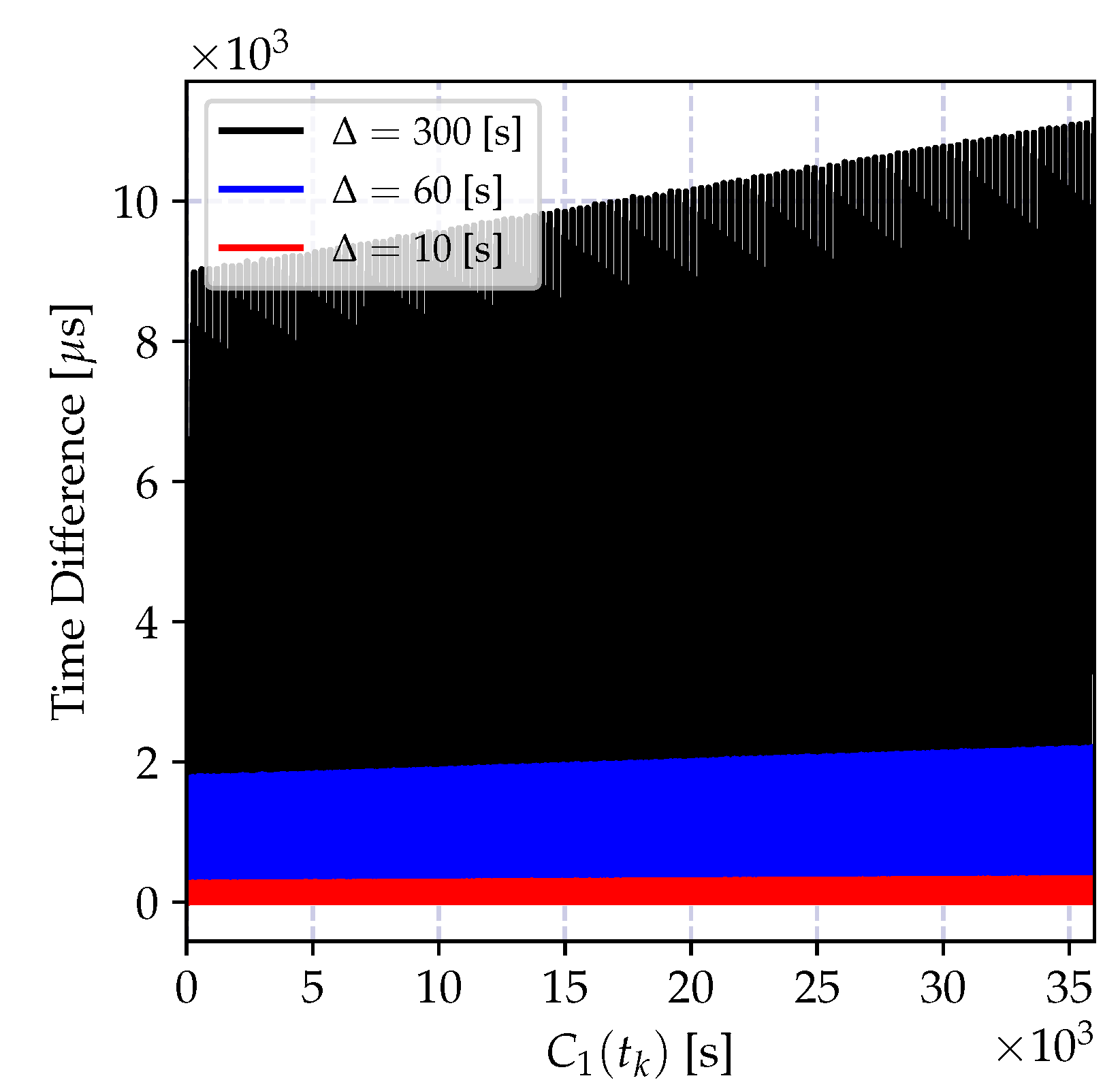
| Offset-only Figure 7 | 10 | 151.32 | 97.28 | 0.037 |
| 60 | 991.99 | 586.87 | 0.039 | |
| 300 | 5025.82 | 2935.20 | 0.040 | |
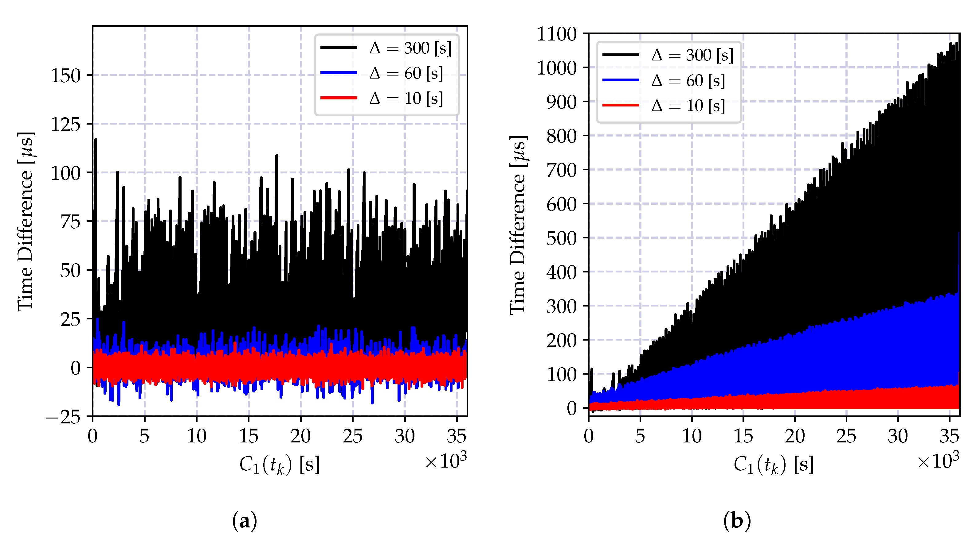
| Batch least squares Figure 8 | 10 | 0.097 | 3.06 | −0.015 |
| 60 | 3.92 | 7.18 | 0.120 | |
| 300 | 94.85 | 29.52 | −0.079 | |
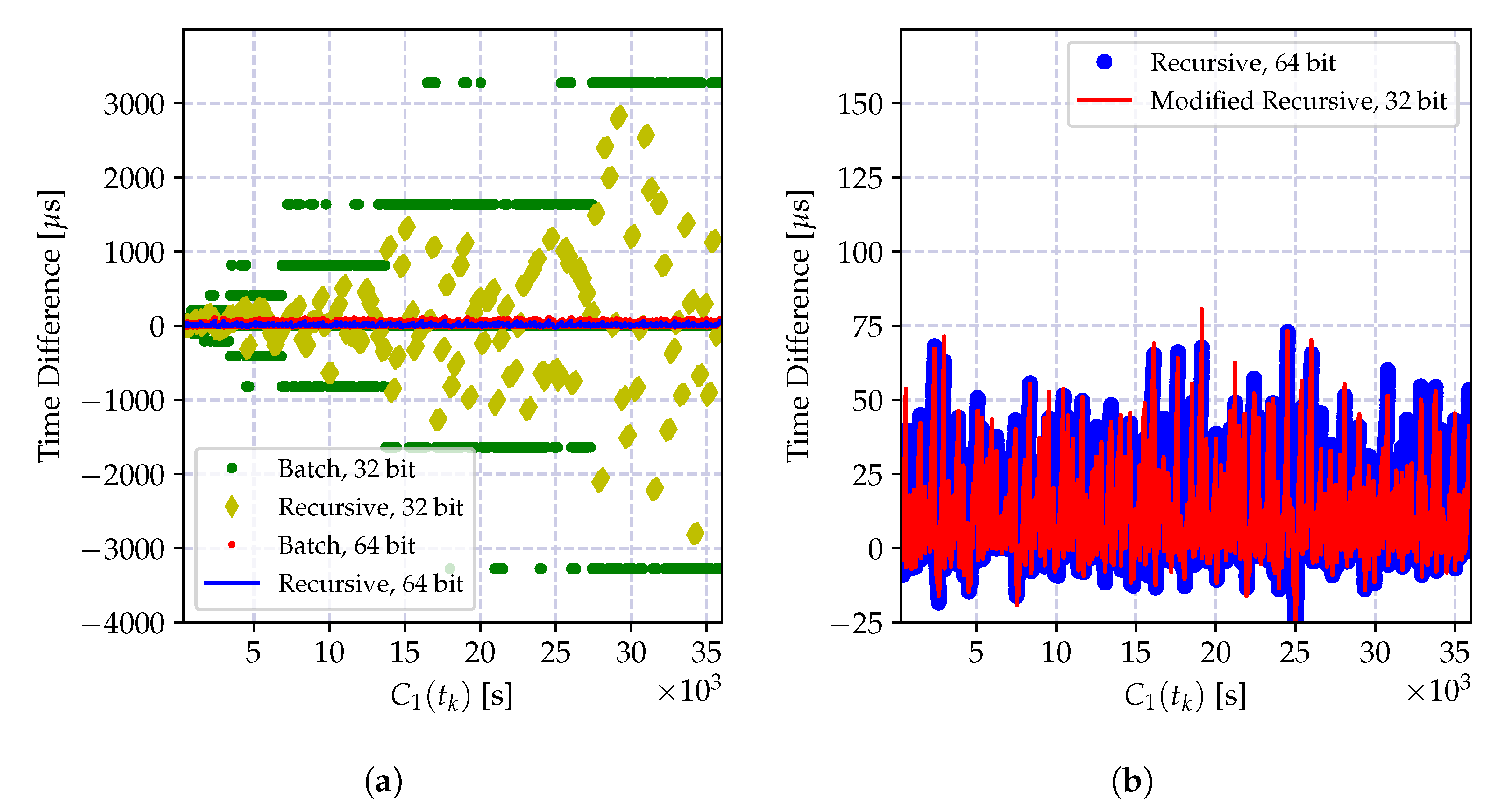
| Batch least squares Figure 9a | 10 | 0.02 | 2.37 | 0.056 |
| 60 | 1.36 | 5.09 | 0.254 | |
| 300 | 33.58 | 23.73 | 0.402 | |
| Recursive MLE Figure 9b | 10 | 15.59 | 13.72 | 0.882 |
| 60 | 93.58 | 75.99 | 0.884 | |
| 300 | 271.79 | 241.65 | 0.979 | |
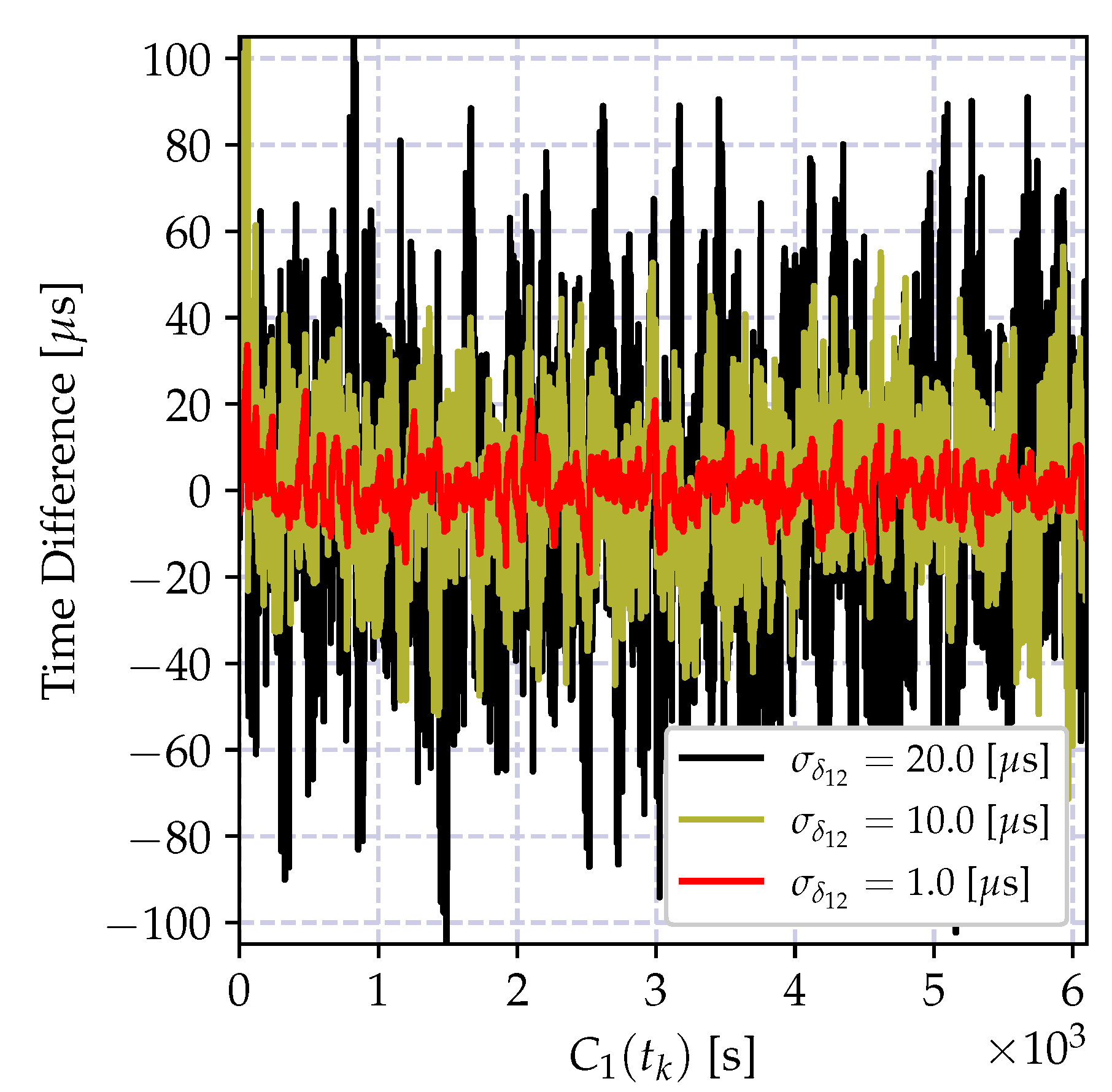
| Weighted recursive MLE Figure 10 | 10 | 0.001 | 2.62 | 0.062 |
| 60 | 0.53 | 5.50 | 0.155 | |
| 300 | 13.40 | 15.35 | 1.073 |
| Estimator | Model | Advantages | Disadvantages |
|---|---|---|---|
| Offset-only estimation [52,53,54] | (17) | A single parameter estimator, which assumes . It is used for adjusting the time using two-way message exchanges. | It has a large modeling error bias, and cannot be used for high accuracy synchronization purposes for low-power networks. |
| Batch least squares estimator [7,55,56,57,58,59,60] | (18) | A simple table-based linear regression estimator. It estimates both skew and offset parameter, and has an acceptable performance. High-precision numerical values are needed to achieve the reported performance. | Its model does not take into account the time variation of clock-skew parameter and oscillator-induced time correlations, which upper bounds the synchronization period. It requires re-calculation of the estimates using all the time values in the table whenever a new time report is available. It treats the clock-skew as an unknown constant. |
| Adaptive skew estimator (Bayesian) [61,62,63] | (19) | A linear state estimator for clock skew, which takes into account the frequency drift. Multiple skew dynamical models can be used simultaneously to account for different practical situations. It assumes dynamics of clock-skew given in Equations (31), (32) or (33) | It does not depend on clock offset, and does not take into account the oscillator-induced correlations into account. Several computational steps of Kalman Filter are required to update its skew estimate. The underlying model requires non-obvious modifications to reach numerically stable estimates. |
| Adaptive skew estimator (Closed-loop) [71,72,73,74] | (19) | Implicit clock skew estimate using PI controller, which resembles PLL loop. Well-known control theoretical tools can be used for adjusting its gains. In its bare form it is equivalent to constant gain Kalman Filter. Adaptive version can be used to adjust its gains on-the-fly. Although not reported, it is expected to be numerically stable. | It does not depend on clock offset, and does not take into account the oscillator-induced correlations into account. A two-step clock discipline algorithm is required. |
| Recursive clock skew estimator [50] | (22) | A computationally efficient (recursive) MLE of the skew. It takes into account oscillator-induced correlations. | It does not depend on clock offset so that two-step clock discipline algorithm is required. It cannot follow the changes in the clock-skew due to frequency drift since it uses all the past time values. |
| Weighted recursive clock skew estimator [This work] | (22) | A computationally efficient (recursive) MLE of the skew. It takes into account oscillator-induced correlations. It supports numerically stable implementation given in Equation (41). It can follow the dynamical variations in the clock skew by limiting number of measurements affecting the estimates. | It does not depend on clock offset so that two step clock discipline algorithm is required. It requires adjusting the forgetting factor for each deployment. This parameter can be selected to include 2–3 reports, since it converges to the correct skew very fast. Numerically stable version requires a constant gain parameter K. This gain can be selected to move significant bits of clock-skew. In practice, can be used. |
| Name | Model | Type | Skew Estimate | Offset Estimate | Bias | Complexity | Sampling |
|---|---|---|---|---|---|---|---|
| Offset-only | Progressive | Batch | (27) | (28) | |||
| Batch least squares | Progressive | Batch | (29a) | (29b) | (30) | Periodic | |
| Batch least squares | Incremental | Batch | (35a) | (35b) | (30) | Periodic | |
| Recursive maximum likelihood | Incremental | Recursive | (38) | (35b) | (30) | A-periodic | |
| Weighted recursive maximum likelihood | Incremental | Recursive | (39a–c) | (35b) | (30) | A-periodic | |
| Numerically-stable recursive maximum likelihood | Incremental | Recursive | (41) | (35b) | (30) | A-periodic |
| Transmitter Delays | Message Processing | Frame Preparation | Software Delay | Encoding Time | Calibration Time | access Time | Transmission Time |
| deterministic | deterministic | random | deterministic | random | random | deterministic | |
| Propagation Delays | propagation time | ||||||
| deterministic | |||||||
| Receiver Delays | reception time | decoding time | byte alignment time | interrupt handling time | |||
| deterministic | deterministic | deterministic | random | ||||
| Synchronization Protocol | Ref. | Messaging Scheme | Multi-Hop Scheme | Description |
|---|---|---|---|---|
| Network Time Protocol (NTP) | [10,11] | two-way | spanning-tree | NTP is the de-fact time synchronization protocol for large networks such as the Internet. The achievable performance is lower than demands of certain applications. |
| IEEE 1588: Precision Time Protocol (PTP) | [13] | two-way | spanning-tree | A high precision time synchronization standard for measurement equipments. Nowadays, it is used in all wired networks applications demanding high precision time synchronization. |
| Time-synchronization Protocol for Sensor Network (TPSN) | [82] | two-way | spanning-tree | TPSN is one of the early multi-hop time synchronization protocols for WSN. It doesn’t compensate for the clock skew. |
| Reference Broadcast Protocol (RBS) | [55] | receiver-receiver | cluster-based | RBS achieves high synchronization accuracy by eliminating transmitter side errors. It enables implementations with minimal modifications in the lower-level software components. |
| Flooding Time Synchronization Protocol (FTSP) | [56] | one-way | spanning-tree | FTSP is widely accepted as the de-facto synchronization protocol for WSN. It achieves high synchronization accuracy using MAC layer timestamping. |
| Flooding with Clock Speed Agreement (FCSA) | [59] | one-way | spanning-tree | FCSA is a slow-flooding based multi-hop solution that extends FTSP. It forces the network to reach clock-speed agreement by combining flooding with a distributed component. |
| Robust Synchronization (R-Sync) | [37] | receiver-only | spanning-tree | R-Sync provides low-power and robust time synchronization protocol for industrial applications. |
| Time Diffusion Protocol (TDP) | [106] | two-way | synchronous diffusion | TDP aims at providing a protocol resilient to node failures and topology changes while taking into account the energy constraints. It is the predecessor of distributed algorithms. |
| Distributed Time Synchronization Protocol (DTSP) | [108] | one-way | distributed | DTSP is the earliest distributed time synchronization method. It uses spatial averaging to converge to a common notion of time. |
| Gradient Time Synchronization Protocol (GTSP) | [109] | one-way | distributed | GTSP is a time synchronization protocol making use of the gradient property. It performs local spatial averaging to reach to a common notion of time. |
| Average Time Synchronization (ATS) | [114] | one-way | distributed | ATS is the first consensus-based time synchronization method for WSN. It tries to reach to the time consensus by converging to a common offset and clock-rate values. |
| Reachback Firefly Algorithm (RFA) | [128] | one-way | distributed | RFA provides a mechanism for network-wide synchronicity, which does not provide a coherent notion of time, but only an option for synchronously executing of a certain task. It is inspired by synchronicity in biological systems. |
Publisher’s Note: MDPI stays neutral with regard to jurisdictional claims in published maps and institutional affiliations. |
© 2020 by the authors. Licensee MDPI, Basel, Switzerland. This article is an open access article distributed under the terms and conditions of the Creative Commons Attribution (CC BY) license (http://creativecommons.org/licenses/by/4.0/).
Share and Cite
Yiğitler, H.; Badihi, B.; Jäntti, R. Overview of Time Synchronization for IoT Deployments: Clock Discipline Algorithms and Protocols. Sensors 2020, 20, 5928. https://doi.org/10.3390/s20205928
Yiğitler H, Badihi B, Jäntti R. Overview of Time Synchronization for IoT Deployments: Clock Discipline Algorithms and Protocols. Sensors. 2020; 20(20):5928. https://doi.org/10.3390/s20205928
Chicago/Turabian StyleYiğitler, Hüseyin, Behnam Badihi, and Riku Jäntti. 2020. "Overview of Time Synchronization for IoT Deployments: Clock Discipline Algorithms and Protocols" Sensors 20, no. 20: 5928. https://doi.org/10.3390/s20205928
APA StyleYiğitler, H., Badihi, B., & Jäntti, R. (2020). Overview of Time Synchronization for IoT Deployments: Clock Discipline Algorithms and Protocols. Sensors, 20(20), 5928. https://doi.org/10.3390/s20205928