Instrumented Cone Penetrometer for Dense Layer Characterization


Abstract
1. Introduction
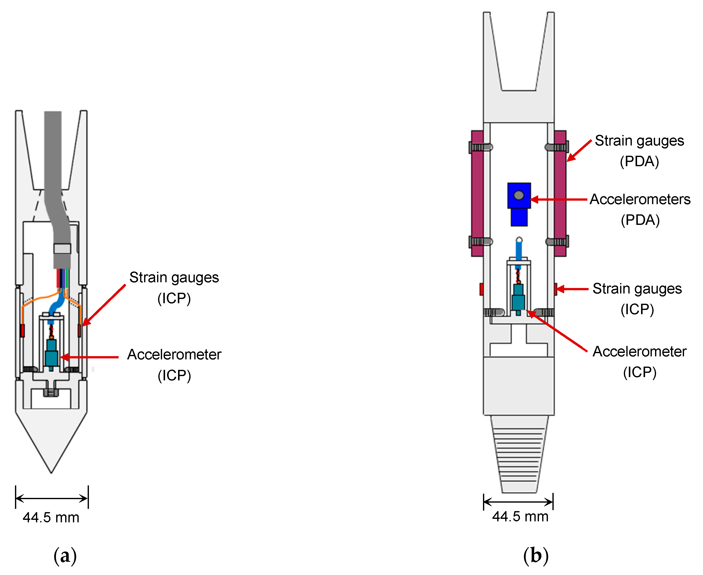
2. Instrumented Cone Penetrometer
2.1. Design
2.2. Data Acquisition System
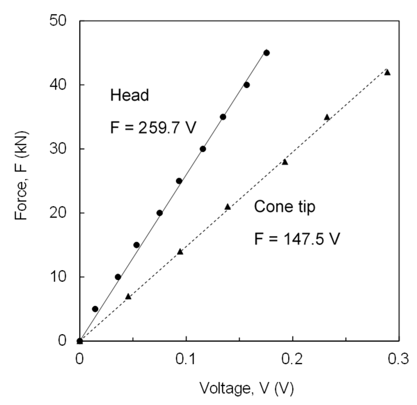
2.3. Calibration
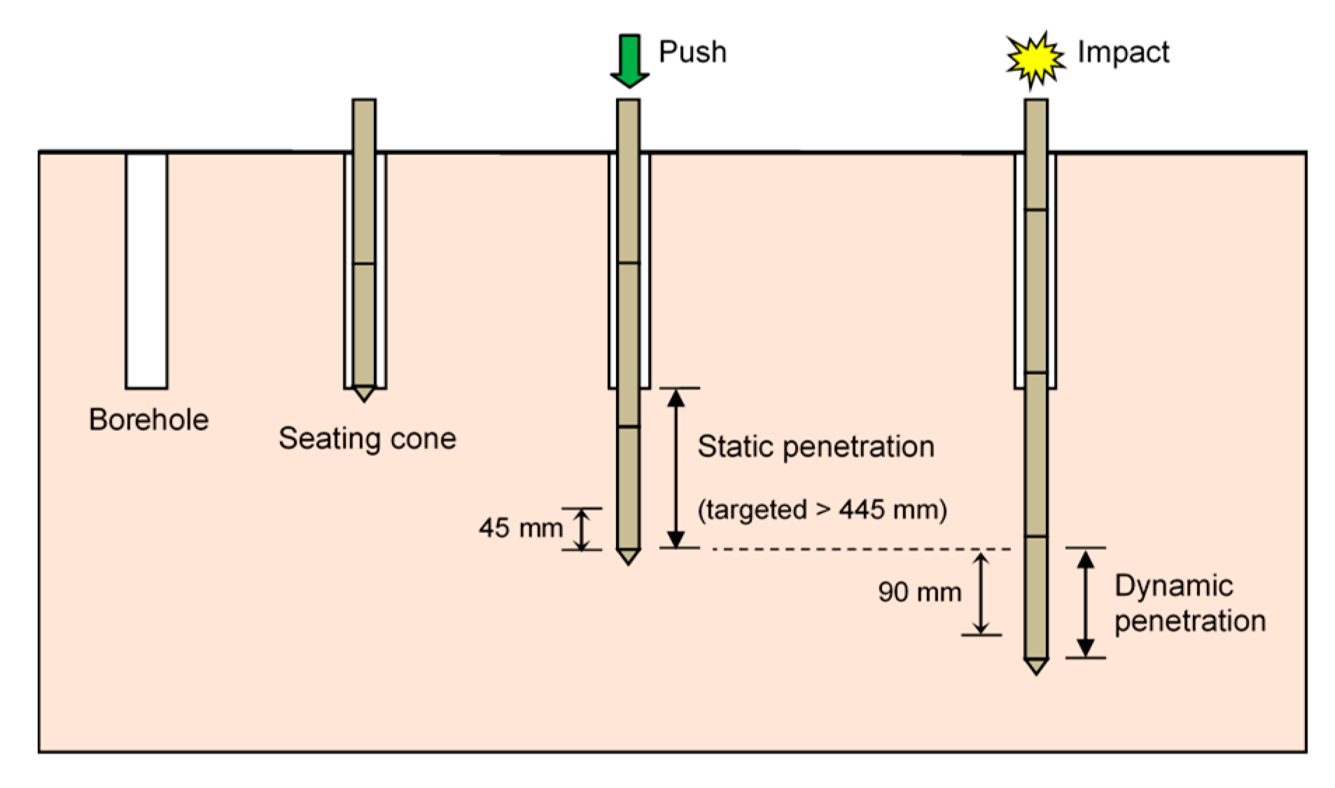
2.4. Test Procedure
3. Results
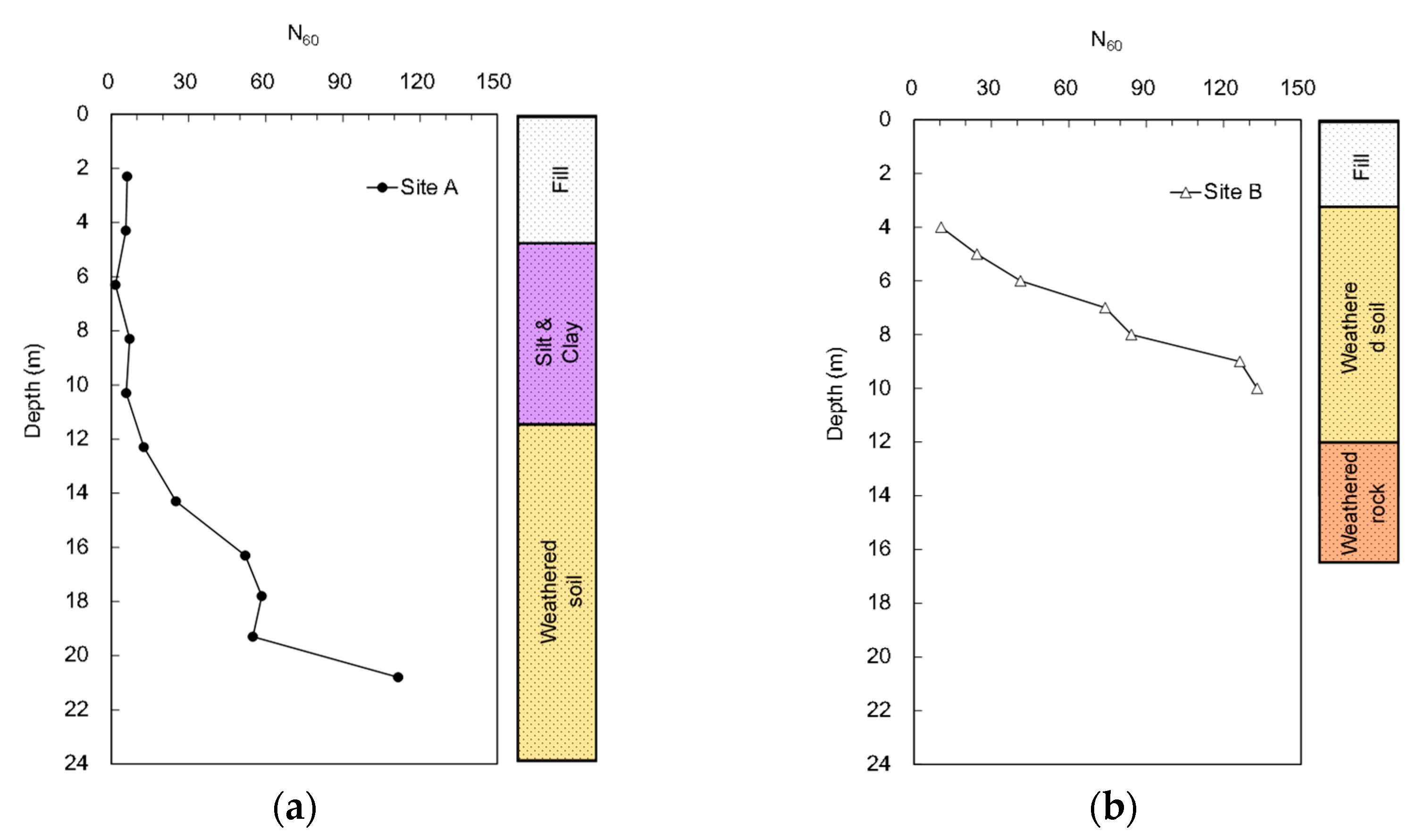
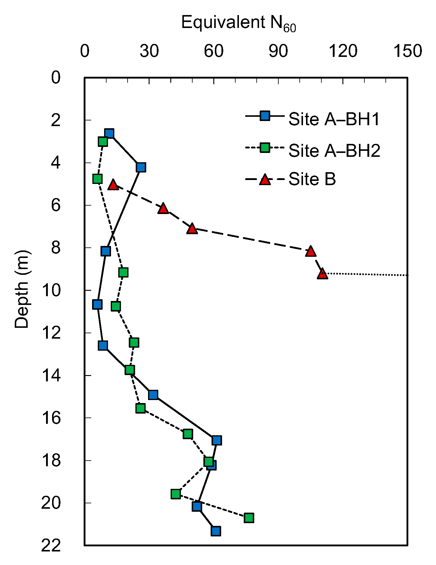
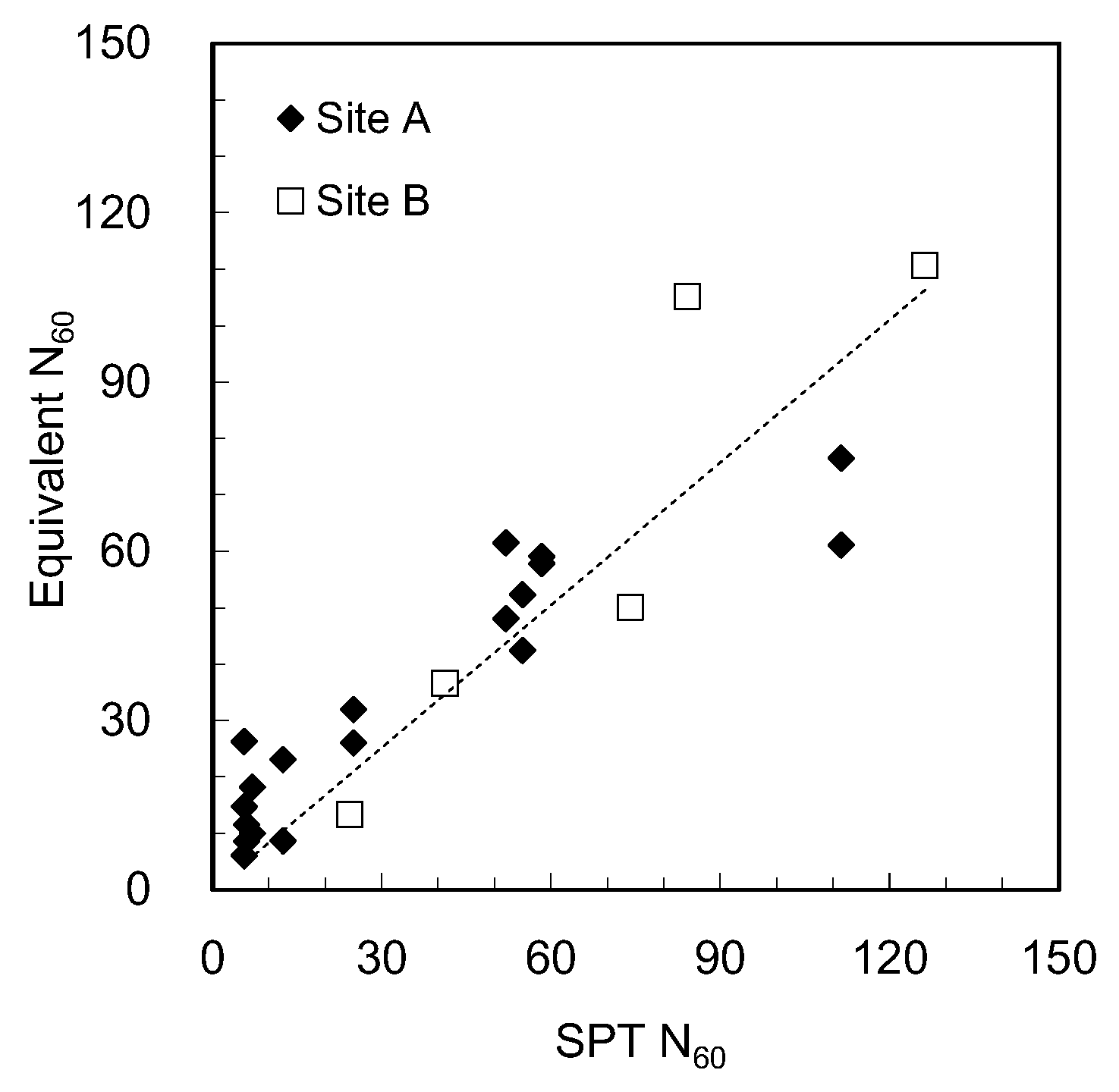
3.1. Standard Penetration Tests
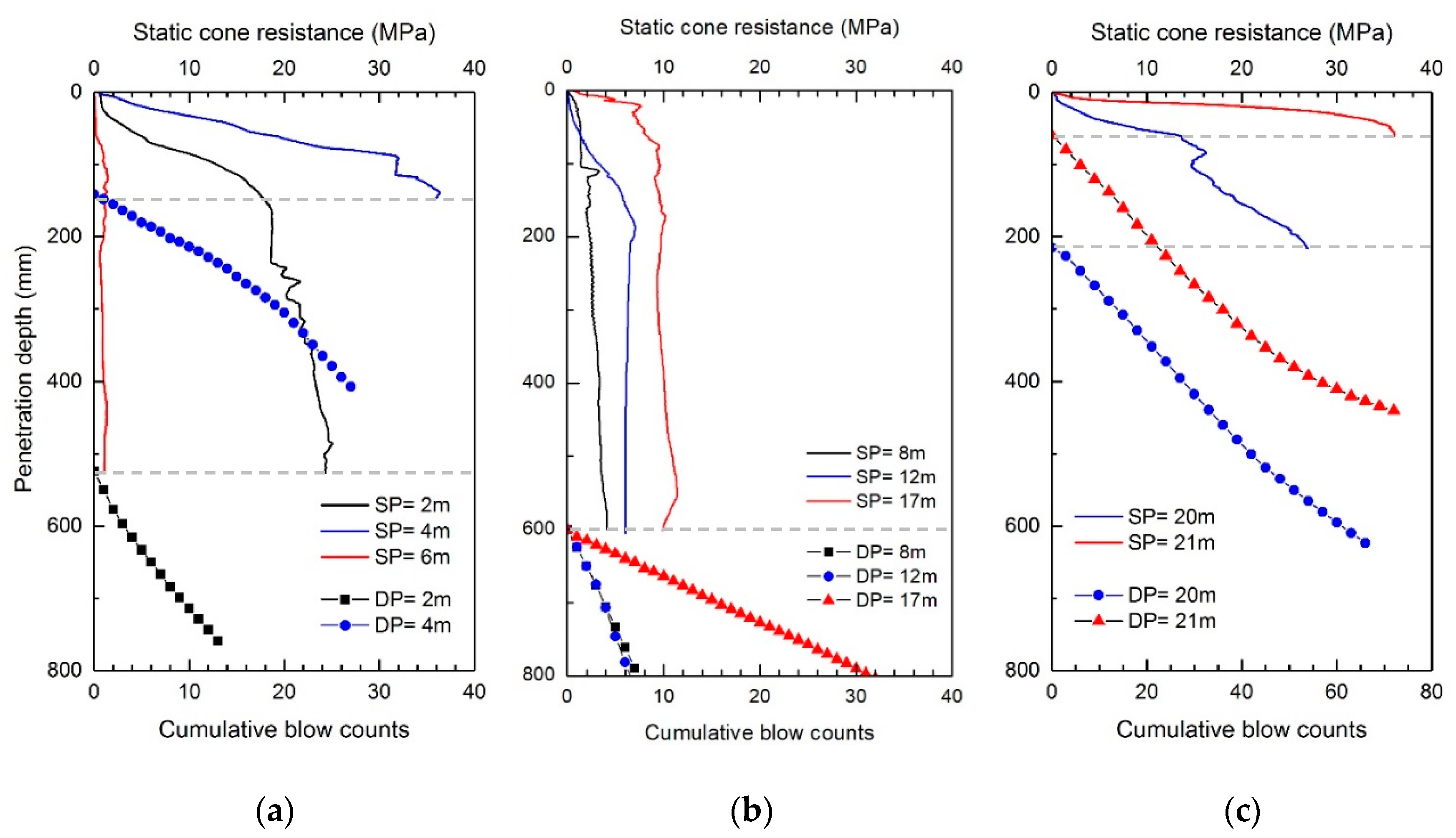
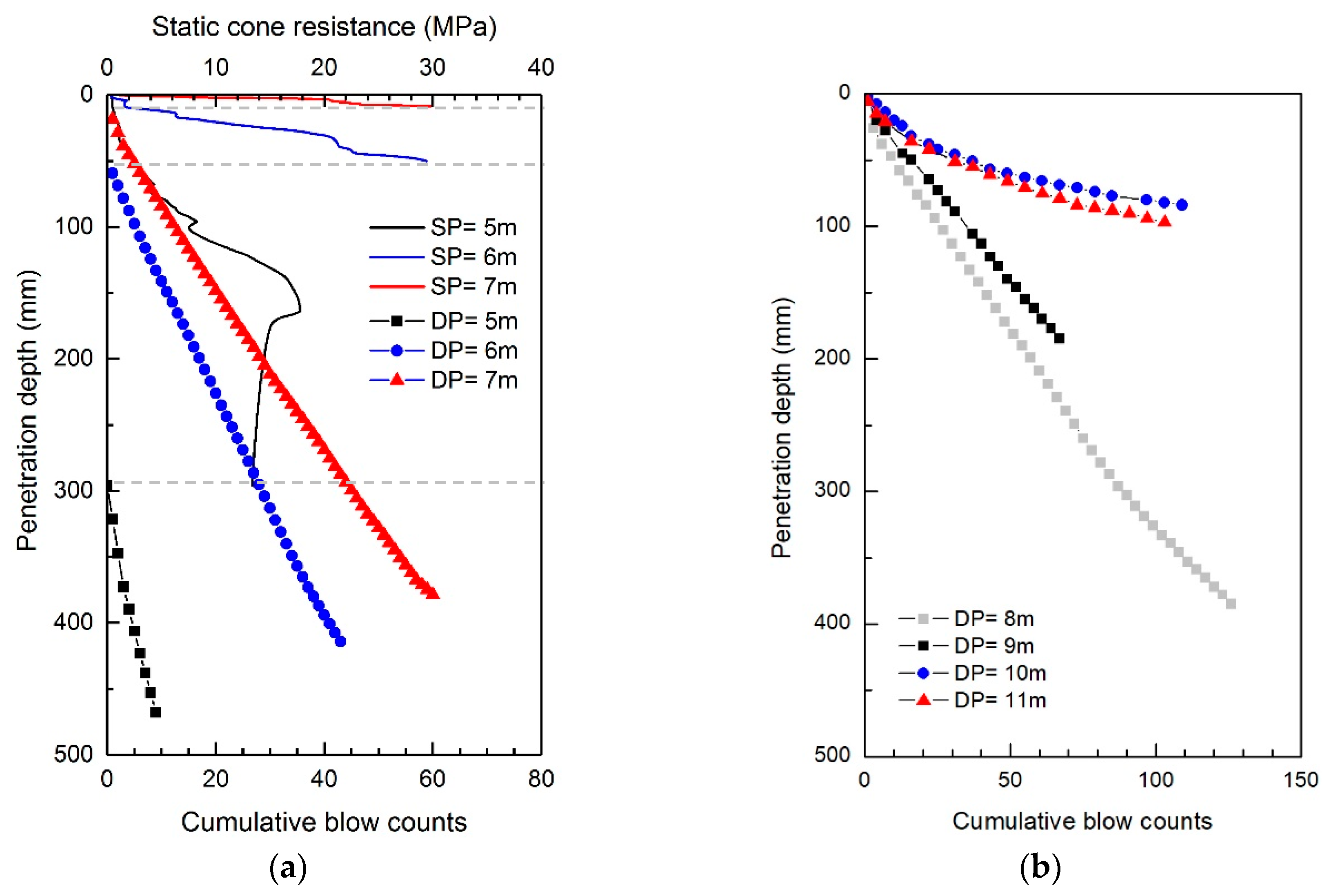
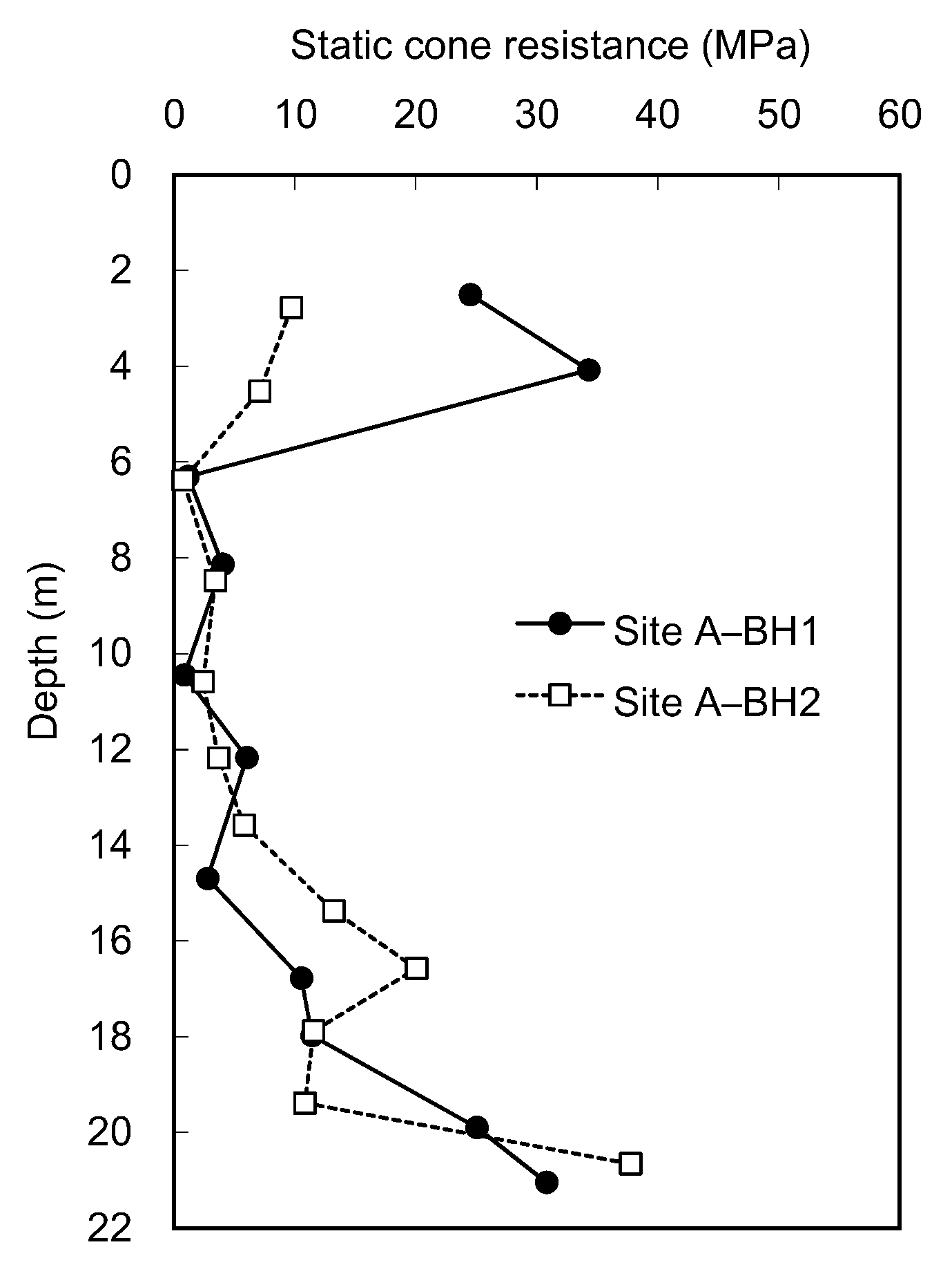
3.2. Static Cone Penetration Tests
3.3. Dynamic Cone Penetration Tests
4. Dynamic Response Analysis
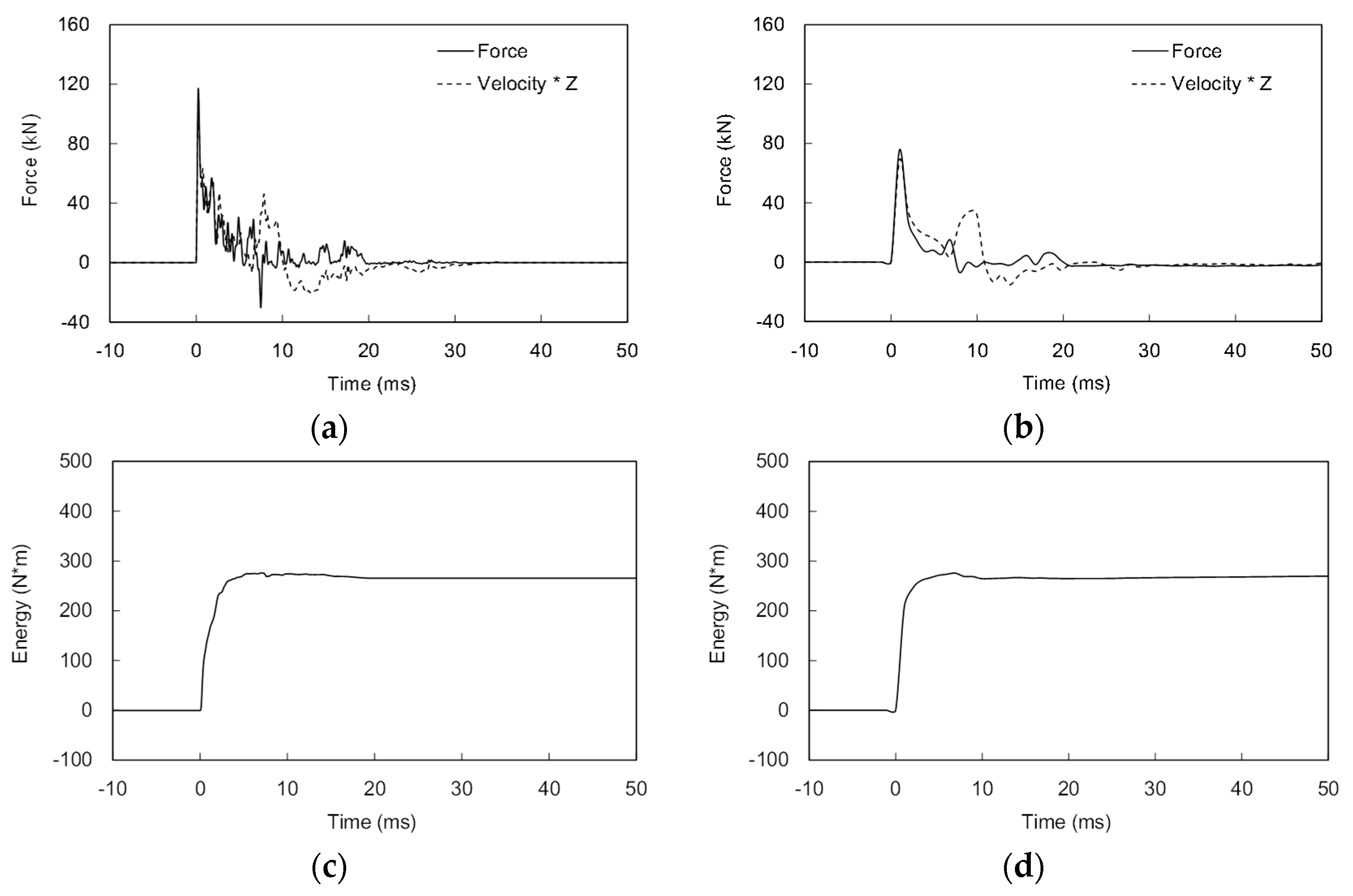
4.1. Instrumentation Verification
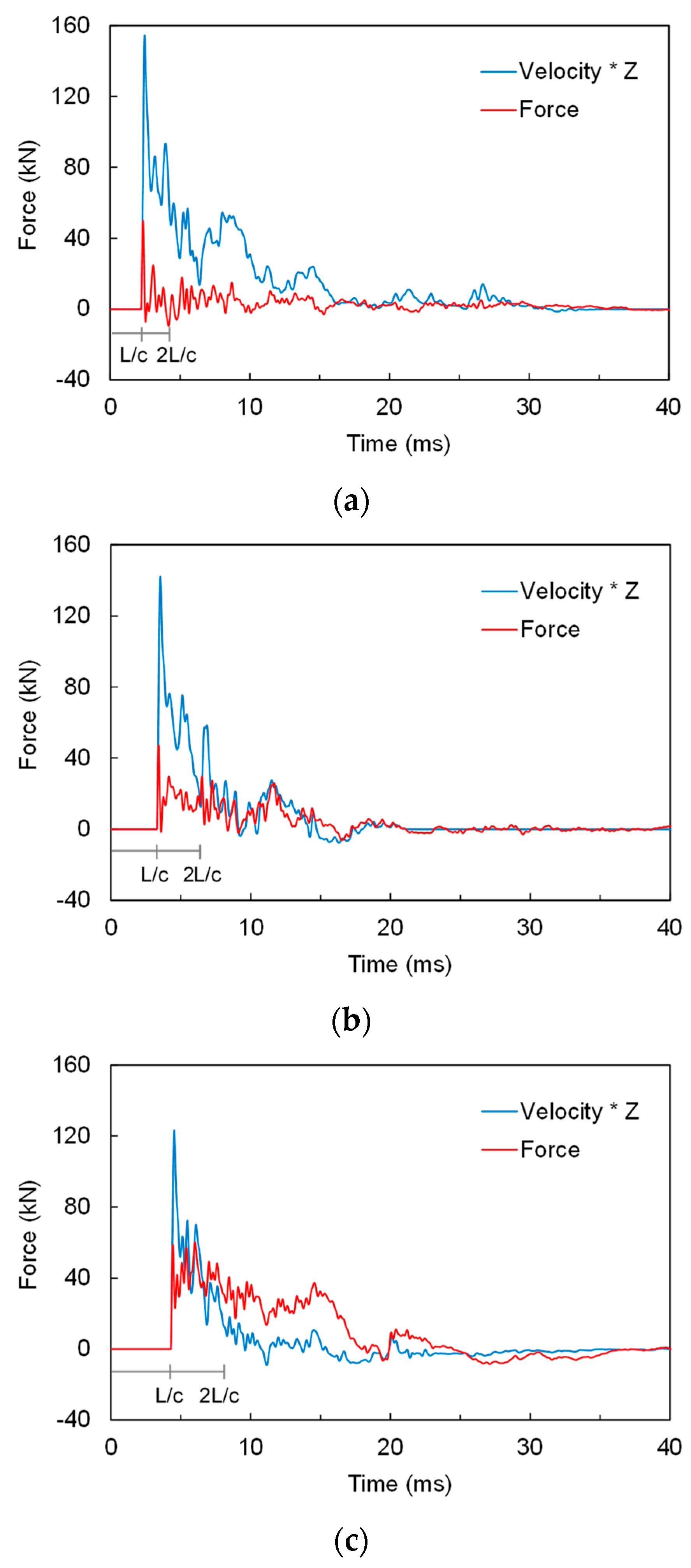
4.2. Force and Velocity
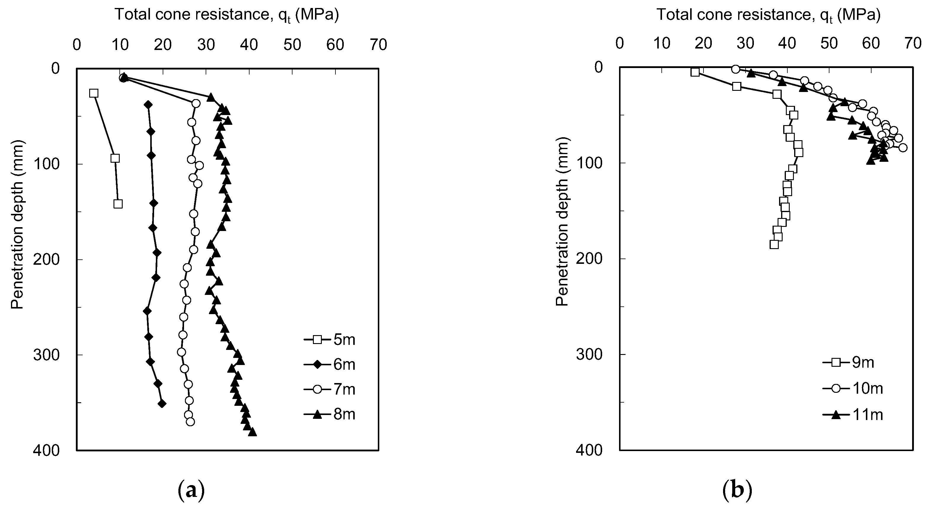
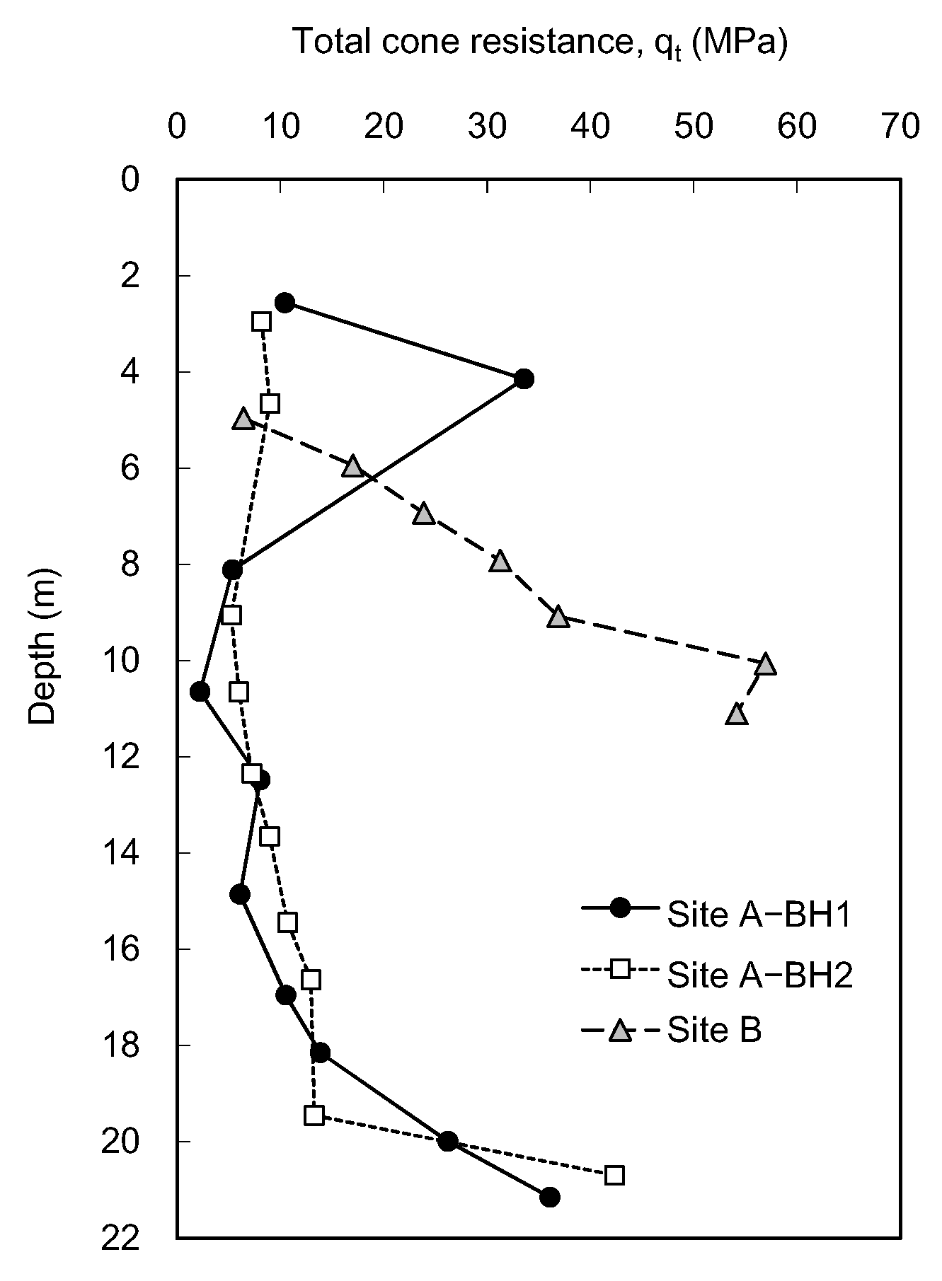
4.3. Total Cone Resistance
5. Correlations with Total Cone Resistance
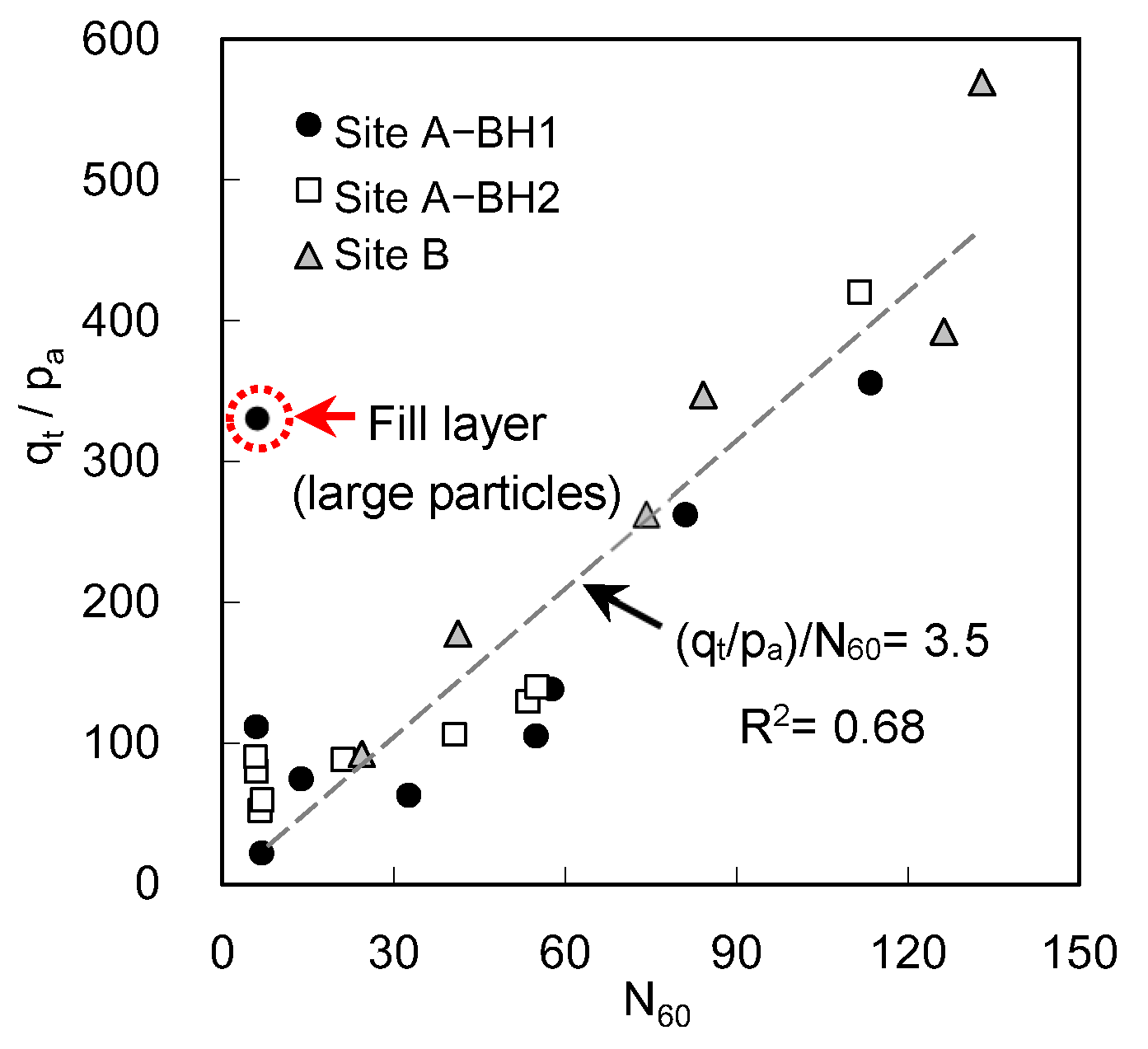
5.1. Total Cone Resistance Versus N Value
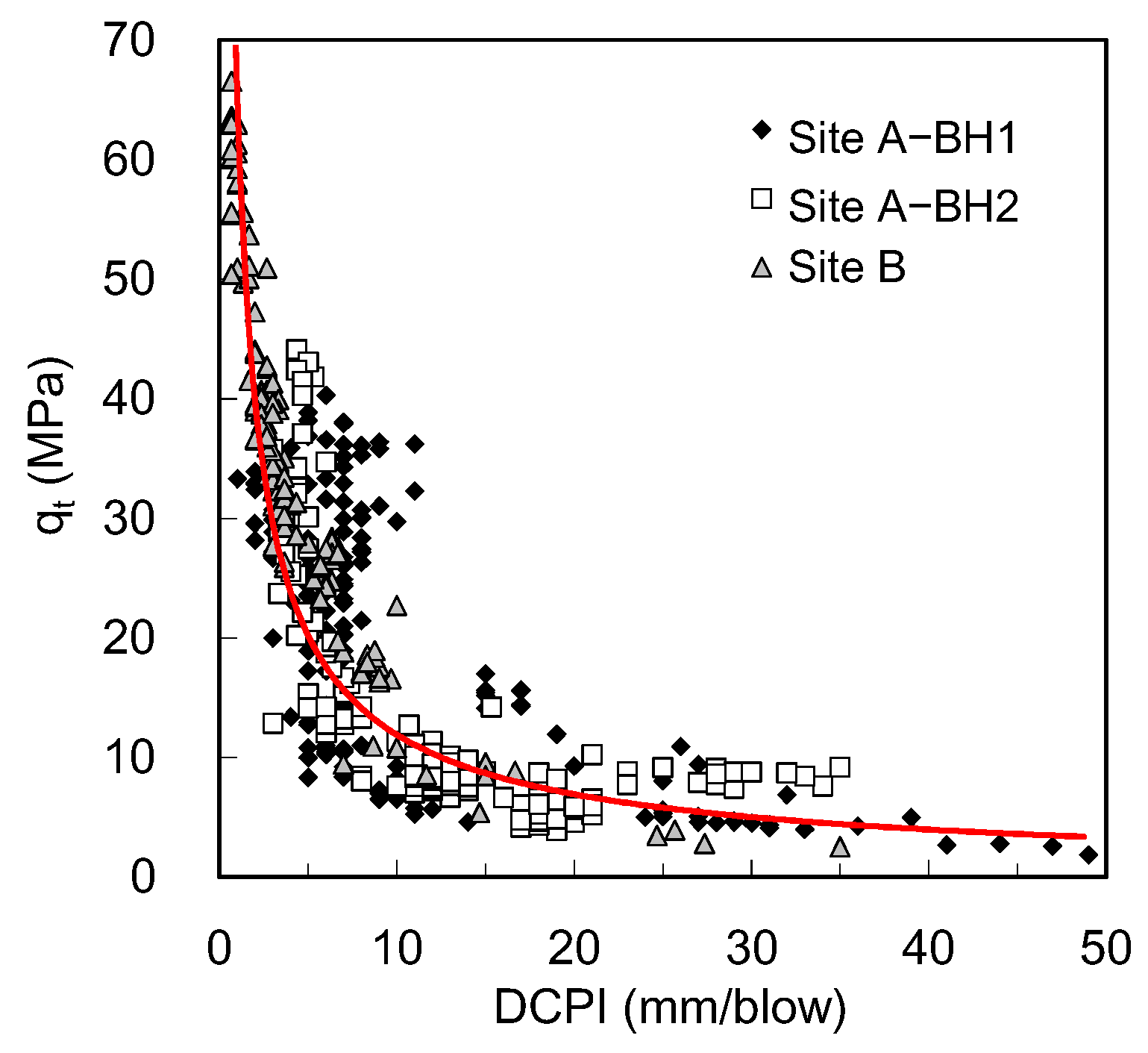
5.2. Total Cone Resistance Versus Dynamic Cone Penetration Index
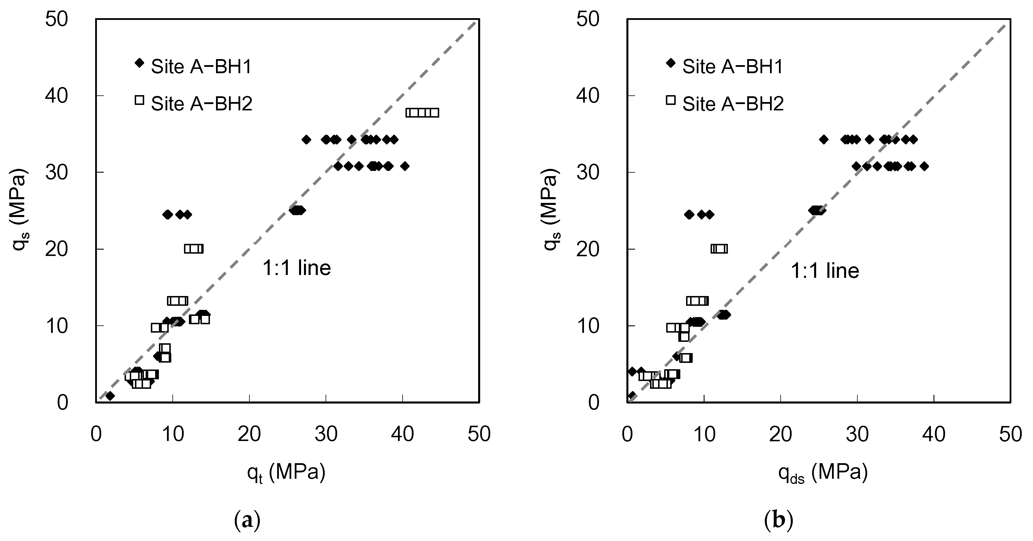
5.3. Total Cone Resistance Versus Static Cone Resistance
6. Summary and Conclusions
Author Contributions
Funding
Acknowledgments
Conflicts of Interest
Notations
| BC100 | () | Cumulative blow count numbers corresponding to the first 100 mm penetration |
| c | (m/s) | Wave velocity through steel |
| CLysm | (kN·s/m) | Damping coefficient |
| CR | () | Factor of rod length |
| D50 | (mm) | Median diameter |
| DCPI | (mm) | Dynamic cone penetration index |
| ER | (%) | Energy ratio |
| Ftip | (kN) | Force detected at the cone tip |
| L | (m) | Total length of the rods at each depth |
| N value | () | Blow count measured in SPT |
| N60 | () | N value corrected by the effects of the rod length and transferred energy |
| pa | (kPa) | Reference stress of 100 kPa |
| qc | (MPa) | Cone tip resistance measured by CPT |
| qd | (MPa) | Dynamic cone resistance estimated from the dynamic cone penetration tests of ICP |
| qds | (MPa) | Static component of the total cone resistance (= qt − qd) in dynamic cone penetration tests |
| qs | (MPa) | Static cone resistance measured from the static cone penetration tests of ICP |
| qt | (MPa) | Total cone resistance estimated from the dynamic cone penetration tests of ICP |
| R | (m) | Radius of the cone penetrometer |
| Vs | (m/s) | Shear wave velocities |
| Vtip | (m/s) | Average velocity measured at the cone tip of the ICP |
| ρ | (kg/m3) | Mass density of the soil |
| υ | () | Poisson’s ratio of the soil |
References
- Skempton, A.W. Standard penetration test procedures and the effects in sands of overburden pressure, relative density, particle size, ageing and overconsolidation. Geotechnique 1986, 36, 425–447. [Google Scholar] [CrossRef]
- Sy, A. Energy Measurements and Correlations of the Standard Penetration Test (SPT) and the Becker Penetration Test (BPT). Ph.D. Thesis, Department of Civil Engineering, University of British Columbia, Vancouver, BC, Canada, 1993. [Google Scholar]
- Campanella, R.G.; Robertson, P.K.; Gillespie, D. Cone penetration testing in deltaic soils. Can. Geotech. J. 1983, 20, 23–35. [Google Scholar] [CrossRef]
- Randolph, M.F.; Hope, S. Effect of cone velocity on cone resistance and excess pore pressures. In Proceedings of the IS Osaka—Engineering Practice and Performance of Soft Deposits, Toyonaka, Japan, 2–4 June 2004. [Google Scholar]
- Kim, K.; Prezzi, M.; Salgado, R.; Lee, W. Effect of penetration rate on cone penetration resistance in saturated clayey soils. J. Geotech. Geoenviron. Eng. 2008, 134, 1142–1153. [Google Scholar] [CrossRef]
- Salgado, R. The mechanics of cone penetration: Contributions from experimental and theoretical studies. Geotech. Geophys. Site Charact. 2012, 4, 131–135. [Google Scholar]
- Schmertmann, J.H. Measurement of in situ shear strength. In Proceedings of the Specialty Conference on In Situ Measurement of Soil Properties, Raleigh, NC, USA, 1–4 June 1975; Volume 2, pp. 57–138. [Google Scholar]
- Schaap, L.H.J.; Zuidberg, H.M. Mechanical and electrical aspects of the electric cone penetrometer tip. In Proceedings of the 2nd European Symposium on Penetration Testing, Amsterdam, The Netherlands, 24–27 May 1982. [Google Scholar]
- Robertson, P.K.; Campanella, R.G.; Wightman, A. SPT-CPT Correlations. J. Geotech. Eng. 1983, 109, 1449–1459. [Google Scholar] [CrossRef]
- Kodicherla, S.P.K.; Nandyala, D.K. Use of CPT and DCP based correlations in characterization of subgrade of a highway in Southern Ethiopia Region. Int. J. Geo-Eng. 2016, 7, 11. [Google Scholar] [CrossRef]
- Mohammadi, S.D.; Nikoudel, M.R.; Rahimi, H.; Khamehchiyan, M. Application of the dynamic cone penetrometer (DCP) for determination of the engineering parameters of sandy soils. Eng. Geol. 2008, 101, 195–203. [Google Scholar] [CrossRef]
- Ilori, A.O. Geotechnical characterization of a highway route alignment with light weight penetrometer (LRS 10), in southeastern Nigeria. Int. J. Geo-Eng. 2015, 6, 7. [Google Scholar] [CrossRef]
- Byun, Y.H.; Lee, J.S. Instrumented dynamic cone penetrometer corrected with transferred energy into a cone tip: A laboratory study. Geotech. Test. J. 2013, 36, 533–542. [Google Scholar] [CrossRef]
- Byun, Y.H.; Yoon, H.K.; Kim, S.Y.; Hong, S.S.; Lee, J.S. Active Layer characterization by instrumented dynamic cone penetrometer in Ny-Alesund, Svalbard. Cold. Regt. Sci. Technol. 2014, 104, 45–53. [Google Scholar] [CrossRef]
- Lee, J.S.; Kim, S.Y.; Hong, W.T.; Byun, Y.H. Assessing subgrade strength using an instrumented dynamic cone penetrometer. Soils Found. 2019, 59, 930–941. [Google Scholar] [CrossRef]
- Kim, S.Y.; Hong, W.T.; Lee, J.S. Role of the coefficient of uniformity on the California bearing ratio, penetration resistance, and small strain stiffness of coarse arctic soils. Cold. Regt. Sci. Technol. 2019, 160, 230–241. [Google Scholar] [CrossRef]
- Kim, S.Y.; Lee, J.S. Energy correction of dynamic cone penetration index for reliable evaluation of shear strength in frozen sand–silt mixtures. Acta Geotech. 2020, 15, 947–961. [Google Scholar] [CrossRef]
- ISO. E.N. 22476-2: Geotechnical Investigation and Testing–Field Testing–Part 2: Dynamic Probing; CEN: Brussels, Belgium, 2005. [Google Scholar]
- Nam, M.S. Improved Design for Drilled Shafts in Rock. Ph.D. Thesis, University of Houston, Houston, TX, USA, 2004. [Google Scholar]
- Smith, J.M.; Miller, G.A. Texas cone penetrometer-pressuremeter correlations for soft rock. In Proceedings of the GeoSupport 2004: Innovation an Cooperation in the Geo-Industry, Orlando, FL, USA, 29–31 January 2004; pp. 441–449. [Google Scholar]
- Texas Department of Transportation. Geotechnical Manual (On-Line Version); Texas Department of Transportation, Bridge Division: Austin, TX, USA, 2006. [Google Scholar]
- Harder, L.F., Jr.; Seed, H.B. Determination of Penetration Resistance for Coarse-Grained Soils Using the Becker Hammer Drill; Report No. UCB/EERC-86/06; College of Engineering, University of California: Berkeley, CA, USA, 1986. [Google Scholar]
- Sy, A.; Campanella, R.G. Standard penetration test energy measurements using a system based upon the personal computer. Can. Geotech. J. 1994, 30, 876–882. [Google Scholar] [CrossRef]
- Ghafghazi, M.; Thurairajah, A.; DeJong, J.T.; Wilson, D.W.; Armstrong, R. Instrumented Becker penetration test for improved characterization of gravelly deposits. In Proceedings of the Geo-Congress 2014: Geo-characterization and Modeling for Sustainability, Atlanta, GA, USA, 23–26 February 2014; pp. 37–46. [Google Scholar]
- Lukiantchuki, J.A.; Esquivel, E.; Bernards, G.P. Interpretation of force and acceleration signals during hammer impact in SPT tests. In Proceedings of the 14th Pan-American Conference on Soil Mechanics Geotechnical Engineering, Toronto, ON, Canada, 2–6 October 2011. [Google Scholar]
- Yoon, H.K.; Lee, J.S. Micro cones configured with full-bridge circuits. Soil Dyn. Earthq. Eng. 2012, 41, 119–127. [Google Scholar] [CrossRef]
- Byun, Y.H.; Hong, W.T.; Lee, J.S. Characterization of railway substructure using a hybrid cone penetrometer. Smart Struct. Syst. 2015, 15, 1085–1101. [Google Scholar] [CrossRef]
- Hong, W.T.; Byun, Y.H.; Kim, S.Y.; Lee, J.S. Cone penetrometer incorporated with dynamic cone penetration method for investigation of track substructures. Smart Struct. Syst. 2016, 18, 197–216. [Google Scholar]
- Lunne, T.; Edismoen, T.; Gillespie, D.; Howland, J.D. Laboratory and field evaluation of cone penetrometers. In Proceedings of the ASCE Specialty Conference In Situ ’86: Use of In Situ Tests in Geotechnical Engineering, Blacksburg, VA, USA, 23–25 June 1986; pp. 714–729. [Google Scholar]
- Lee, C.; Kim, R.; Lee, J.S.; Lee, W. Quantitative assessment of temperature effect on cone resistance. Bull. Eng. Geol. Environ. 2013, 72, 3–13. [Google Scholar] [CrossRef]
- Treen, C.R.; Robertson, P.K.; Woeller, D.J. Cone penetration testing in stiff glacial soils using a downhole cone penetrometer. Can. Geotech. J. 1992, 29, 448–455. [Google Scholar] [CrossRef]
- Salgado, R. The Engineering of Foundations; McGraw-Hill: New York, NY, USA, 2008. [Google Scholar]
- Bustamante, M.; Gianeselli, L. Pile bearing capacity prediction by means of static penetrometer CPT. In Proceedings of the 2nd European Symposium on Penetration Testing, Amsterdam, The Netherlands, 24–27 May 1982; pp. 493–500. [Google Scholar]
- Schnaid, F.; Odebrecht, E.; Rocha, M.M. On the mechanics of dynamic penetration tests. Geomech. Geoengin. Int. J. 2007, 2, 137–146. [Google Scholar] [CrossRef]
- Schnaid, F.; Odebrecht, E.; Rocha, M.M.; Bernardes, G.P. Prediction of soil properties from the concepts of energy transfer in dynamic penetration tests. J. Geotech. Geoenviron. Eng. 2009, 135, 1092–1100. [Google Scholar] [CrossRef]
- Schnaid, F.; Lourenco, D.; Odebrecht, E. Interpretation of static and dynamic penetration tests in coarse-grained soils. Géotech. Lett. 2017, 7, 113–118. [Google Scholar] [CrossRef]
- Kianirad, E. Development and Testing of a Portable In-Situ Near-Surface Soil Characterization System. Ph.D. Thesis, Northeastern University, Boston, MA, USA, 2011. [Google Scholar]
- Schmertmann, J.H.; Palacios, A. Energy dynamics of SPT. J. Geotech. Eng. Div. 1979, 105, 909–926. [Google Scholar]
- Kulhawy, F.H.; Mayne, P.W. Manual on Estimating Soil Properties for Foundation Design (No. EPRI-EL-6800); Electric Power Research Institute: Palo Alto, CA, USA, 1990. [Google Scholar]
- Lysmer, J.; Richart, F.E. Dynamic response of footing to vertical loading. J. Soil Mech. Found. Div. 1966, 92, 65–91. [Google Scholar]
- Baldi, G.; Bellotti, R.; Ghionna, V.N.; Jamiolkowski, M.; Lopresti, D.C.F. Modulus of sands from CPTs and DMTs. In Proceedings of the 12th International Conference on Soil Mechanics and Foundation Engineering, Rio de Janeiro, Brazil, 13–18 August 1989; pp. 165–170. [Google Scholar]
- Mayne, P.W.; Rix, G.J. Correlations between shear wave velocity and cone tip resistance in clays. Soils Found. 1995, 35, 165–170. [Google Scholar] [CrossRef]


| Depth (m) | N60 | Sampling Depth (m) | Specific Gravity Gs | Median Diameter D50 (mm) | Gradation Coefficient Cc | Uniformity Coefficient Cu | Water Content wc (%) | Liquid Limit LL (%) | Plastic Limit PL (%) | Plasticity Index PI (%) | US CS * |
|---|---|---|---|---|---|---|---|---|---|---|---|
| 0–3.3 | 6 | 2.3 | 2.88 | 1.64 | 0.31 | 26.76 | 14 | - | - | - | SP |
| 3.3–5.3 | 6 | 4.3 | 2.72 | 4.12 | 0.94 | 38.3 | 16 | - | - | - | SP |
| 5.3–7.3 | 2 | 6.3 | 2.68 | 0.13 | 0.71 | 2.54 | 37 | 31 | 27 | 4 | ML |
| 7.3–9.3 | 7 | 8.3 | 2.72 | 0.49 | 0.77 | 3.43 | 26 | 45 | 23 | 22 | CL |
| 9.3–11.3 | 6 | 10.3 | 2.71 | 0.34 | 0.59 | 3.12 | 32 | 39 | 28 | 11 | CL |
| 11.3–13.3 | 13 | 12.3 | 2.72 | 0.33 | 0.7 | 2.61 | 32 | 34 | 29 | 5 | SM |
| 13.3–15.3 | 25 | 14.3 | 2.66 | 0.42 | 0.84 | 3.08 | 24 | 33 | 27 | 6 | SM |
| 15.3–17.1 | 52 | 16.3 | 2.68 | 0.49 | 0.8 | 3.52 | 28 | 33 | 27 | 6 | SM |
| 17.1–18.6 | 58 | 17.8 | 2.65 | 0.58 | 0.9 | 3.54 | 18 | 32 | 26 | 6 | SM |
| 18.6–20.1 | 55 | 19.3 | 2.59 | 0.5 | 0.86 | 3.09 | 24 | 32 | 28 | 4 | SM |
| 20.1–21.6 | 112 | 20.8 | 2.66 | 0.56 | 0.85 | 3.07 | 14 | 26 | 23 | 3 | SM |
| a | b | R2 | |
|---|---|---|---|
| Site A | 72.33 | −0.773 | 0.60 |
| Site B | 65.23 | −0.641 | 0.82 |
| Entire | 70.87 | −0.757 | 0.73 |
| Depth (m) | Shear Wave Velocity Vs (m/s) | Damping Coefficient CLysm (kN·s/m) | Average Velocity at Cone Tip Vtip (m/s) | Average Dynamic Cone Resistance qd (MPa) | ||||
|---|---|---|---|---|---|---|---|---|
| BH1 | BH2 | BH1 | BH2 | BH1 | BH2 | BH1 | BH2 | |
| 0–3.3 | 120.1 | 117.0 | 0.53 | 0.52 | 3.73 | 5.10 | 1.27 | 1.69 |
| 3.3–5.3 | 192.8 | 162.4 | 0.95 | 0.80 | 2.69 | 3.14 | 1.63 | 1.61 |
| 7.3–8.3 | 516.4 | 233.2 | 2.30 | 1.04 | 3.21 | - | 4.76 | - |
| 8.3–9.3 | 292.8 | 280.2 | 1.31 | 1.25 | - | 2.93 | - | 2.36 |
| 10.3–11.3 | 199.7 | 241.1 | 0.89 | 1.08 | 3.30 | 2.42 | 1.89 | 1.67 |
| 12.3–13.3 | 206.8 | 200.1 | 0.91 | 0.88 | 2.70 | 2.30 | 1.59 | 1.31 |
| 13.3–14.3 | 211.4 | 215.1 | 0.93 | 0.95 | - | 2.18 | - | 1.33 |
| 14.3–15.3 | 217.3 | 233.7 | 0.96 | 1.03 | 2.38 | - | 1.47 | - |
| 15.3–16.1 | 233.6 | 248.4 | 1.06 | 1.13 | - | 2.11 | - | 1.53 |
| 16.1–17.1 | 247.2 | 262.4 | 1.15 | 1.22 | 1.87 | 1.22 | 1.38 | 0.96 |
| 17.1–18.6 | 263.4 | 260.0 | 1.23 | 1.21 | 1.80 | - | 1.42 | - |
| 18.6–20.1 | 280.2 | 258.7 | 1.34 | 1.24 | 1.71 | - | 1.47 | - |
© 2020 by the authors. Licensee MDPI, Basel, Switzerland. This article is an open access article distributed under the terms and conditions of the Creative Commons Attribution (CC BY) license (http://creativecommons.org/licenses/by/4.0/).
Share and Cite
Lee, J.-S.; Byun, Y.-H. Instrumented Cone Penetrometer for Dense Layer Characterization. Sensors 2020, 20, 5782. https://doi.org/10.3390/s20205782
Lee J-S, Byun Y-H. Instrumented Cone Penetrometer for Dense Layer Characterization. Sensors. 2020; 20(20):5782. https://doi.org/10.3390/s20205782
Chicago/Turabian StyleLee, Jong-Sub, and Yong-Hoon Byun. 2020. "Instrumented Cone Penetrometer for Dense Layer Characterization" Sensors 20, no. 20: 5782. https://doi.org/10.3390/s20205782
APA StyleLee, J.-S., & Byun, Y.-H. (2020). Instrumented Cone Penetrometer for Dense Layer Characterization. Sensors, 20(20), 5782. https://doi.org/10.3390/s20205782