Applying Fully Convolutional Architectures for Semantic Segmentation of a Single Tree Species in Urban Environment on High Resolution UAV Optical Imagery

 ,
,  , , , , , and
Abstract
1. Introduction
2. Materials and Methods
2.1. Study Area and Data Acquisition
2.2. Semantic Segmentation Methods
2.2.1. U-Net
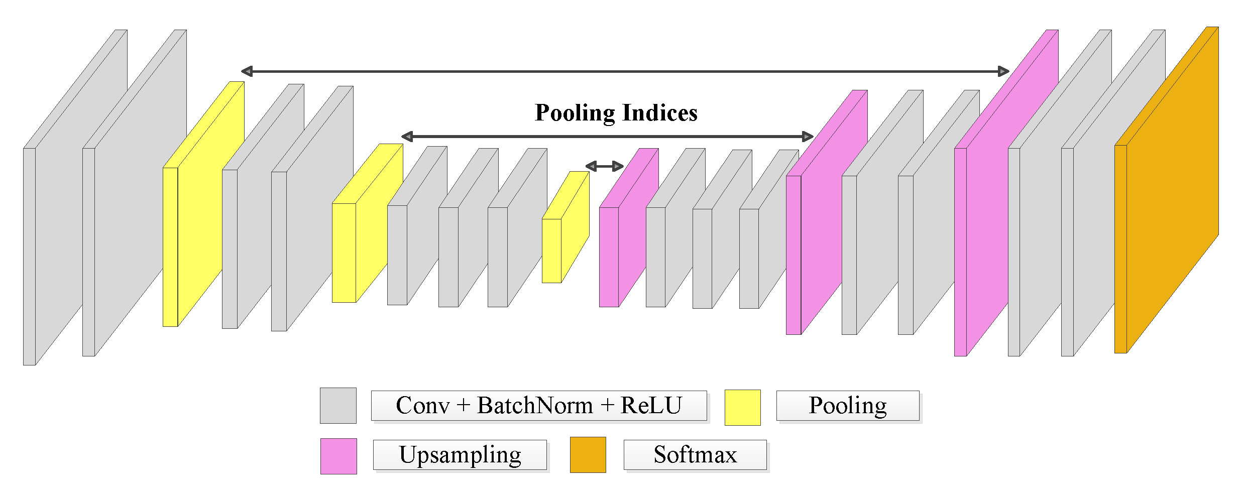
2.2.2. SegNet
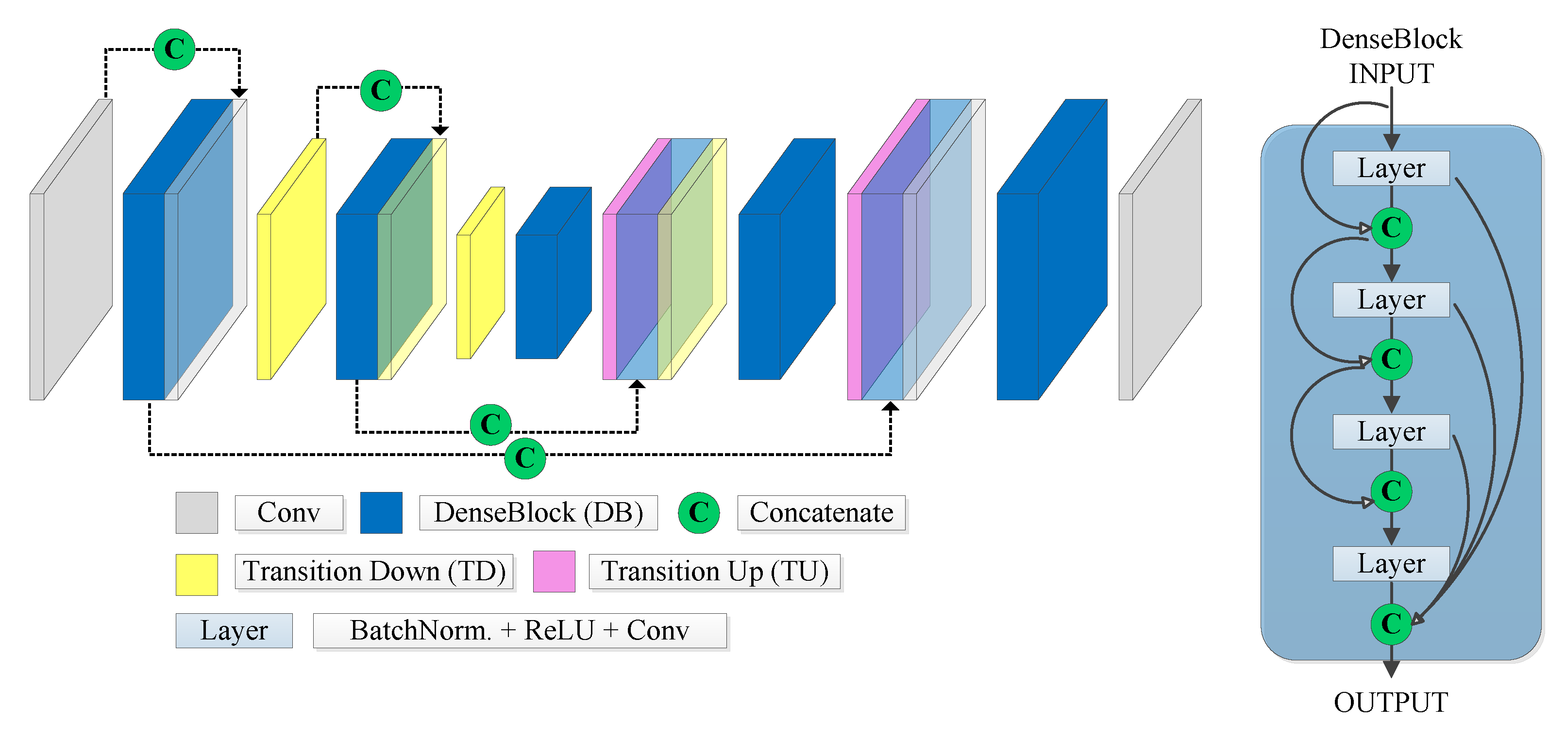
2.2.3. FC-DenseNet
2.2.4. DeepLabv3+ with the Xception Backbone
2.2.5. DeepLabv3+ with the MobileNetV2 Backbone
2.3. Conditional Random Field
2.4. Experimental Evaluation
2.5. Evaluation Metrics
3. Results and Discussion
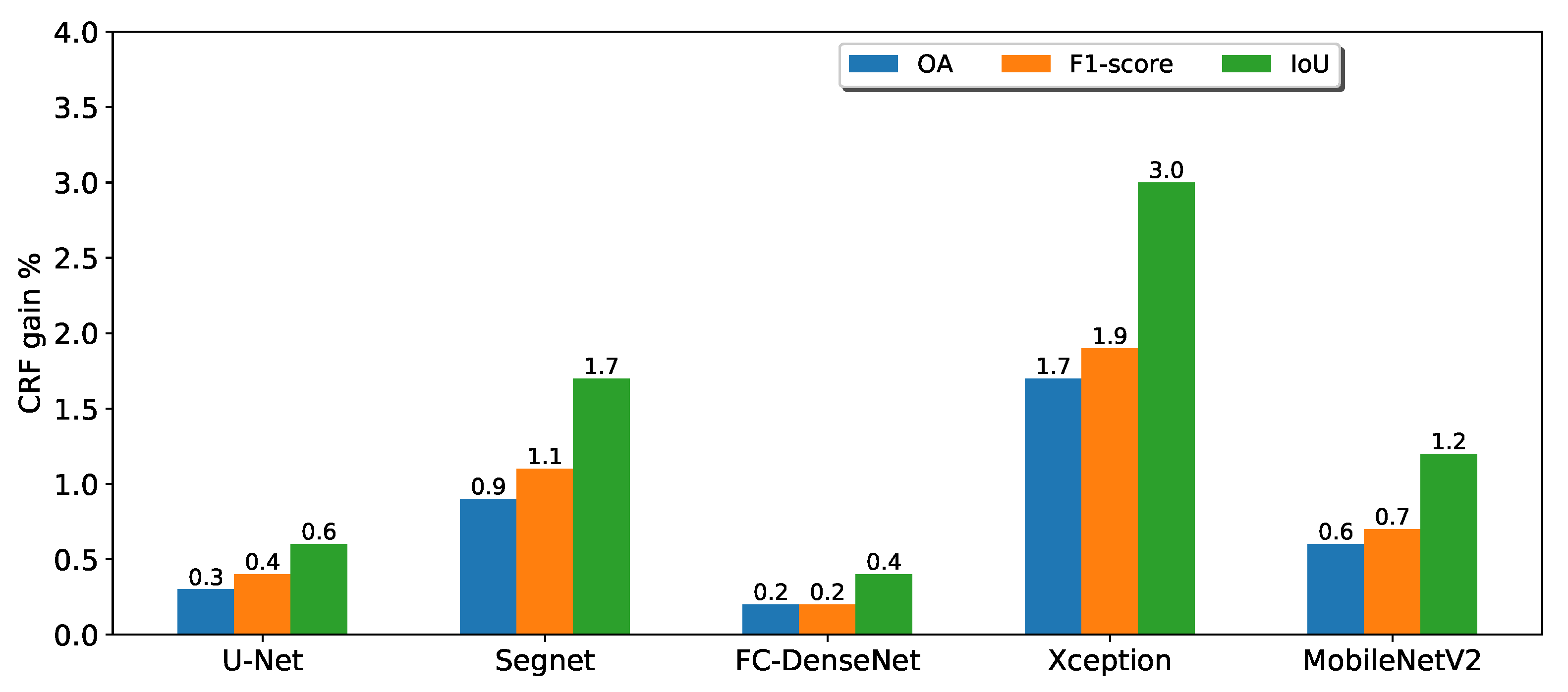
3.1. Performance Evaluation
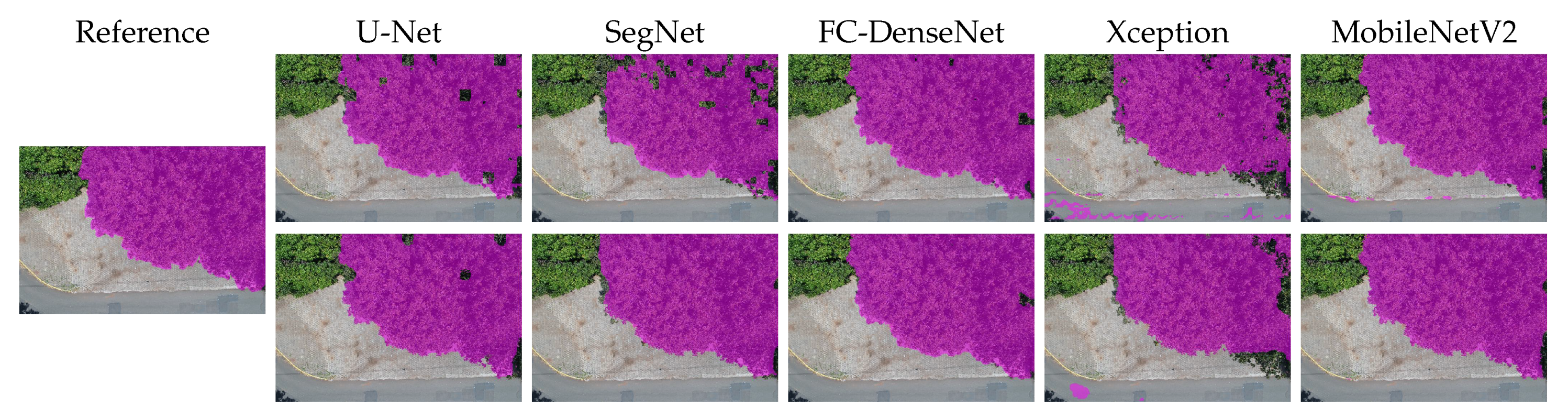
3.2. Visual Analysis
3.3. Computational Complexity
4. Conclusions and Research Perspective
Author Contributions
Funding
Conflicts of Interest
Appendix A

| True | True | ||||||
|---|---|---|---|---|---|---|---|
| Cumbaru | Background | Cumbaru | Background | ||||
| (+) | (−) | (+) | (−) | ||||
| Predicted | Cumbaru (+) | 0.42 | 0.02 | Predicted | Cumbaru (+) | 0.43 | 0.02 |
| Background (−) | 0.02 | 0.54 | Background (−) | 0.02 | 0.53 | ||
| True | True | ||||||
|---|---|---|---|---|---|---|---|
| Cumbaru | Background | Cumbaru | Background | ||||
| (+) | (−) | (+) | (−) | ||||
| Predicted | Cumbaru (+) | 0.39 | 0.05 | Predicted | Cumbaru (+) | 0.4 | 0.04 |
| Background (−) | 0.05 | 0.51 | Background (−) | 0.04 | 0.52 | ||
| True | True | ||||||
|---|---|---|---|---|---|---|---|
| Cumbaru | Background | Cumbaru | Background | ||||
| (+) | (−) | (+) | (−) | ||||
| Predicted | Cumbaru (+) | 0.41 | 0.01 | Predicted | Cumbaru (+) | 0.41 | 0.01 |
| Background (−) | 0.02 | 0.56 | Background (−) | 0.02 | 0.56 | ||
| True | True | ||||||
|---|---|---|---|---|---|---|---|
| Cumbaru | Background | Cumbaru | Background | ||||
| (+) | (−) | (+) | (−) | ||||
| Predicted | Cumbaru (+) | 0.37 | 0.02 | Predicted | Cumbaru (+) | 0.38 | 0.01 |
| Background (−) | 0.09 | 0.52 | Background (−) | 0.08 | 0.53 | ||
| True | True | ||||||
|---|---|---|---|---|---|---|---|
| Cumbaru | Background | Cumbaru | Background | ||||
| (+) | (−) | (+) | (−) | ||||
| Predicted | Cumbaru (+) | 0.41 | 0.02 | Predicted | Cumbaru (+) | 0.41 | 0.02 |
| Background (−) | 0.03 | 0.54 | Background (−) | 0.03 | 0.54 | ||
References
- Alonzo, M.; Bookhagen, B.; Roberts, D. Urban tree species mapping using hyperspectral and LiDAR data fusion. Remote Sens. Environ. 2014, 148, 70–83. [Google Scholar] [CrossRef]
- Cheng, G.; Han, J. A survey on object detection in optical remote sensing images. ISPRS J. Photogramm. Remote Sens. 2016, 117, 11–28. [Google Scholar] [CrossRef]
- Fassnacht, F.; Latifi, H.; Stereńczak, K.; Modzelewska, A.; Lefsky, M.; Waser, L.T.; Straub, C.; Ghosh, A. Review of studies on tree species classification from remotely sensed data. Remote Sens. Environ. 2016, 186, 64–87. [Google Scholar] [CrossRef]
- Brockhaus, J.A.; Khorram, S. A comparison of SPOT and Landsat-TM data for use in conducting inventories of forest resources. Int. J. Remote Sens. 1992, 13, 3035–3043. [Google Scholar] [CrossRef]
- Rogan, J.; Miller, J.; Stow, D.; Franklin, J.; Levien, L.; Fischer, C. Land-Cover Change Monitoring with Classification Trees Using Landsat TM and Ancillary Data. Photogramm. Eng. Remote Sens. 2003, 69, 793–804. [Google Scholar] [CrossRef]
- Salovaara, K.; Thessler, S.; Malik, R.; Tuomisto, H. Classification of Amazonian Primary Rain Forest Vegetation using Landsat ETM+Satellite Imagery. Remote Sens. Environ. 2005, 97, 39–51. [Google Scholar] [CrossRef]
- Johansen, K.; Phinn, S. Mapping Structural Parameters and Species Composition of Riparian Vegetation Using IKONOS and Landsat ETM+ Data in Australian Tropical Savannahs. Photogramm. Eng. Remote Sens. 2006, 72, 71–80. [Google Scholar] [CrossRef]
- Clark, M.; Roberts, D.; Clark, D. Hyperspectral discrimination of tropical rain forest tree species at leaf to crown scales. Remote Sens. Environ. 2005, 96, 375–398. [Google Scholar] [CrossRef]
- Zhen, Z.; Quackenbush, L.J.; Zhang, L. Trends in Automatic Individual Tree Crown Detection and Delineation—Evolution of LiDAR Data. Remote Sens. 2016, 8, 333. [Google Scholar] [CrossRef]
- Wang, K.; Wang, T.; Liu, X. A Review: Individual Tree Species Classification Using Integrated Airborne LiDAR and Optical Imagery with a Focus on the Urban Environment. Forests 2018, 10, 1. [Google Scholar] [CrossRef]
- Jensen, R.R.; Hardin, P.J.; Bekker, M.; Farnes, D.S.; Lulla, V.; Hardin, A. Modeling urban leaf area index with AISA+ hyperspectral data. Appl. Geogr. 2009, 29, 320–332. [Google Scholar] [CrossRef]
- Gong, P.; Howarth, P. An Assessment of Some Factors Influencing Multispectral Land-Cover Classification. Photogramm. Eng. Remote Sens. 1990, 56, 597–603. [Google Scholar]
- Chenari, A.; Erfanifard, Y.; Dehghani, M.; Pourghasemi, H.R. Woodland Mapping at Single-Tree Levels Using Object-Oriented Classification of Unmanned Aerial Vehicle (UAV) Images. In Proceedings of the 2017 International Archives of the Photogrammetry, Remote Sensing and Spatial Information Sciences, Tehran, Iran, 7–10 October 2017. [Google Scholar]
- Zhang, C.; Kovacs, J. The application of small unmanned aerial systems for precision agriculture: A review. Precis. Agric. 2012, 13, 693–712. [Google Scholar] [CrossRef]
- Honkavaara, E.; Saari, H.; Kaivosoja, J.; Pölönen, I.; Hakala, T.; Litkey, P.; Mäkynen, J.; Pesonen, L. Processing and Assessment of Spectrometric, Stereoscopic Imagery Collected Using a Lightweight UAV Spectral Camera for Precision Agriculture. Remote Sens. 2013, 5, 5006–5039. [Google Scholar] [CrossRef]
- Anderson, K.; Gaston, K. Lightweight unmanned aerial vehicles will revolutionize spatial ecology. Front. Ecol. Environ. 2013, 11, 138–146. [Google Scholar] [CrossRef]
- Koh, L.; Wich, S. Dawn of drone ecology: low-cost autonomous aerial vehicles for conservation. Trop. Conserv. Sci. 2012, 5, 121–132. [Google Scholar] [CrossRef]
- Salamí, E.; Barrado, C.; Pastor, E. UAV Flight Experiments Applied to the Remote Sensing of Vegetated Areas. Remote Sens. 2014, 6, 11051–11081. [Google Scholar] [CrossRef]
- Feng, X.; Li, P. A Tree Species Mapping Method from UAV Images over Urban Area Using Similarity in Tree-Crown Object Histograms. Remote Sens. 2019, 11, 1982. [Google Scholar] [CrossRef]
- Baena, S.; Moat, J.; Whaley, O.Q.; Boyd, D.S. Identifying species from the air: UAVs and the very high resolution challenge for plant conservation. PLoS ONE 2017, 12, e0188714. [Google Scholar] [CrossRef]
- Santos, A.A.D.; Marcato Junior, J.; Araújo, M.S.; Di Martini, D.R.; Tetila, E.C.; Siqueira, H.L.; Aoki, C.; Eltner, A.; Matsubara, E.T.; Pistori, H.; et al. Assessment of CNN-Based Methods for Individual Tree Detection on Images Captured by RGB Cameras Attached to UAVs. Sensors 2019, 19, 3595. [Google Scholar] [CrossRef]
- Mottaghi, R.; Chen, X.; Liu, X.; Cho, N.G.; Lee, S.W.; Fidler, S.; Urtasun, R.; Yuille, A. The Role of Context for Object Detection and Semantic Segmentation in the Wild. In Proceedings of the 2014 IEEE Conference on Computer Vision and Pattern Recognition, Columbus, OH, USA, 24–27 June 2014. [Google Scholar]
- Chen, X.; Mottaghi, R.; Liu, X.; Fidler, S.; Urtasun, R.; Yuille, A.L. Detect What You Can: Detecting and Representing Objects using Holistic Models and Body Parts. arXiv 2014, arXiv:1406.2031. [Google Scholar]
- Badrinarayanan, V.; Handa, A.; Cipolla, R. SegNet: A Deep Convolutional Encoder-Decoder Architecture for Robust Semantic Pixel-Wise Labelling. arXiv 2015, arXiv:1505.07293. [Google Scholar]
- Chen, L.; Papandreou, G.; Kokkinos, I.; Murphy, K.; Yuille, A.L. DeepLab: Semantic Image Segmentation with Deep Convolutional Nets, Atrous Convolution, and Fully Connected CRFs. IEEE Trans. Pattern Anal. Mach. Intell. 2018, 40, 834–848. [Google Scholar] [CrossRef] [PubMed]
- Li, Y.; Zhang, H.; Xue, X.; Jiang, Y.; Shen, Q. Deep learning for remote sensing image classification: A survey. Wiley Interdiscip. Rev. Data Min. Knowl. Discov. 2018, 8, e1264. [Google Scholar] [CrossRef]
- Li, W.; Fu, H.; Yu, L.; Cracknell, A. Deep Learning Based Oil Palm Tree Detection and Counting for High-Resolution Remote Sensing Images. Remote Sens. 2017, 9, 22. [Google Scholar] [CrossRef]
- Weinstein, B.G.; Marconi, S.; Bohlman, S.; Zare, A.; White, E. Individual Tree-Crown Detection in RGB Imagery Using Semi-Supervised Deep Learning Neural Networks. Remote Sens. 2019, 11, 1309. [Google Scholar] [CrossRef]
- Natesan, S.; Armenakis, C.; Vepakomma, U. Resnet-based tree species classification using uav images. In Proceedings of the 2019 International Archives of the Photogrammetry, Remote Sensing and Spatial Information Sciences, Enschede, The Netherlands, 10–14 June 2019. [Google Scholar]
- Onishi, M.; Ise, T. Automatic classification of trees using a UAV onboard camera and deep learning. arXiv 2018, arXiv:1804.10390. [Google Scholar]
- Baatz, M.; Schape, A. Multiresolution segmentation: an optimization approach for high quality multi scale image segmentation. Angew. Geogr. Informationsverarbeitung 2000, XII, 12–23. [Google Scholar]
- Shanmugamani, R. Deep Learning for Computer Vision: Expert Techniques to Train Advanced Neural Networks Using TensorFlow and Keras; Packt Publishing Ltd.: Birmingham, UK, 2018. [Google Scholar]
- Long, J.; Shelhamer, E.; Darrell, T. Fully Convolutional Networks for Semantic Segmentation. arXiv 2014, arXiv:1411.4038. [Google Scholar]
- Ronneberger, O.; Fischer, P.; Brox, T. U-Net: Convolutional Networks for Biomedical Image Segmentation. arXiv 2015, arXiv:1505.04597. [Google Scholar]
- He, K.; Gkioxari, G.; Dollár, P.; Girshick, R. Mask r-cnn. In Proceedings of the 2017 IEEE International Conference on Computer Vision and Pattern Recognition, Venice, Italy, 22–29 October 2017; pp. 2961–2969. [Google Scholar]
- Liu, Y.; Piramanayagam, S.; Monteiro, S.T.; Saber, E. Dense semantic labeling of very-high-resolution aerial imagery and lidar with fully-convolutional neural networks and higher-order CRFs. In Proceedings of the 2017 IEEE International Conference on Computer Vision and Pattern Recognition, Venice, Italy, 22–29 October 2017; pp. 1561–1570. [Google Scholar]
- Liu, Y.; Fan, B.; Wang, L.; Bai, J.; Xiang, S.; Pan, C. Semantic labeling in very high resolution images via a self-cascaded convolutional neural network. ISPRS J. Photogramm. Remote Sens. 2018, 145, 78–95. [Google Scholar] [CrossRef]
- Chen, L.; Papandreou, G.; Schroff, F.; Adam, H. Rethinking Atrous Convolution for Semantic Image Segmentation. arXiv 2017, arXiv:1706.05587. [Google Scholar]
- Wagner, F.H.; Sanchez, A.; Tarabalka, Y.; Lotte, R.G.; Ferreira, M.P.; Aidar, M.P.; Gloor, E.; Phillips, O.L.; Aragao, L.E. Using the U-net convolutional network to map forest types and disturbance in the Atlantic rainforest with very high resolution images. Remote Sens. Ecol. Conserv. 2019, 5, 360–375. [Google Scholar] [CrossRef]
- Kattenborn, T.; Eichel, J.; Fassnacht, F.E. Convolutional Neural Networks enable efficient, accurate and fine-grained segmentation of plant species and communities from high-resolution UAV imagery. Sci. Rep. 2019, 9, 1–9. [Google Scholar] [CrossRef] [PubMed]
- Arakaki, A.A.H.; Scheidt, G.N.; Portella, A.C.; Arruda, E.J.A.D.; Costa, R.B.D. O baru (Dipteryx alata Vog.) como alternativa de sustentabilidade em área de fragmento florestal do Cerrado, no Mato Grosso do Sul. Interaςões (Campo Grande) 2009, 10, 31–39. [Google Scholar] [CrossRef]
- Liu, Y.; Nguyen, D.; Deligiannis, N.; Ding, W.; Munteanu, A. Hourglass-ShapeNetwork Based Semantic Segmentation for High Resolution Aerial Imagery. Remote Sens. 2017, 9, 522. [Google Scholar] [CrossRef]
- Volpi, M.; Tuia, D. Dense semantic labeling of sub-decimeter resolution images with convolutional neural networks. arXiv 2016, arXiv:1608.00775. [Google Scholar]
- Garcia-Garcia, A.; Orts-Escolano, S.; Oprea, S.; Villena-Martinez, V.; Rodríguez, J.G. A Review on Deep Learning Techniques Applied to Semantic Segmentation. arXiv 2017, arXiv:1704.06857. [Google Scholar]
- Jégou, S.; Drozdzal, M.; Vázquez, D.; Romero, A.; Bengio, Y. The One Hundred Layers Tiramisu: Fully Convolutional DenseNets for Semantic Segmentation. In Proceedings of the 2017 IEEE Conference on Computer Vision and Pattern Recognition, Venice, Italy, 22–29 October 2017; pp. 1175–1183. [Google Scholar]
- Huang, G.; Liu, Z.; Weinberger, K.Q. Densely Connected Convolutional Networks. arXiv 2016, arXiv:1608.06993. [Google Scholar]
- Hai, J.; Qiao, K.; Chen, J.J.; Tan, H.; Xu, J.; Zeng, L.; Shi, D.; Yan, B. Fully Convolutional DenseNet with Multiscale Context for Automated Breast Tumor Segmentation. J. Health. Eng. 2019, 2019, 522. [Google Scholar] [CrossRef]
- Chen, L.; Zhu, Y.; Papandreou, G.; Schroff, F.; Adam, H. Encoder-Decoder with Atrous Separable Convolution for Semantic Image Segmentation. arXiv 2018, arXiv:1802.02611. [Google Scholar]
- Guo, Y.; Li, Y.; Feris, R.S.; Wang, L.; Rosing, T. Depthwise Convolution is All You Need for Learning Multiple Visual Domains. arXiv 2019, arXiv:1902.00927. [Google Scholar] [CrossRef]
- Chollet, F. Xception: Deep Learning with Depthwise Separable Convolutions. arXiv 2016, arXiv:1610.02357. [Google Scholar]
- Hariharan, B.; Arbeláez, P.A.; Girshick, R.B.; Malik, J. Hypercolumns for Object Segmentation and Fine-grained Localization. arXiv 2014, arXiv:1411.5752. [Google Scholar]
- Zhang, T.; Jiang, S.; Zhao, Z.; Dixit, K.; Zhou, X.; Hou, J.; Zhang, Y.; Yan, C. Rapid and robust two-dimensional phase unwrapping via deep learning. Opt. Express 2019, 27, 23173–23185. [Google Scholar] [CrossRef] [PubMed]
- Sandler, M.; Howard, A.G.; Zhu, M.; Zhmoginov, A.; Chen, L. Inverted Residuals and Linear Bottlenecks: Mobile Networks for Classification, Detection and Segmentation. arXiv 2018, arXiv:1801.04381. [Google Scholar]
- Liu, Y.; Ren, Q.; Geng, J.; Ding, M.; Li, J. Efficient Patch-Wise Semantic Segmentation for Large-Scale Remote Sensing Images. Sensors 2018, 18, 3232. [Google Scholar] [CrossRef]
- Chen, L.C.; Papandreou, G.; Kokkinos, I.; Murphy, K.; Yuille, A.L. Semantic Image Segmentation with Deep Convolutional Nets and Fully Connected CRFs. arXiv 2014, arXiv:1412.7062. [Google Scholar]
- Krähenbühl, P.; Koltun, V. Efficient Inference in Fully Connected CRFs with Gaussian Edge Potentials. In Proceedings of the 24th International Conference on Neural Information Processing Systems; Curran Associates Inc.: Dutchess County, NY, USA, 2011; pp. 109–117. [Google Scholar]
- Chollet, F. Keras. 2015. Available online: https://keras.io (accessed on 20 January 2020).
- Kingma, D.P.; Ba, J. Adam: A Method for Stochastic Optimization. arXiv 2014, arXiv:1412.6980. [Google Scholar]
- Sokolova, M.; Japkowicz, N.; Szpakowicz, S. Beyond Accuracy, F-Score and ROC: A Family of Discriminant Measures for Performance Evaluation. In AI 2006: Advances in Artificial Intelligence; Springer: Berlin/Heidelberg, Germany, 2006; Volume 4304, pp. 1015–1021. [Google Scholar]
- Rezatofighi, S.H.; Tsoi, N.; Gwak, J.; Sadeghian, A.; Reid, I.D.; Savarese, S. Generalized Intersection over Union: A Metric and A Loss for Bounding Box Regression. arXiv 2019, arXiv:1902.09630. [Google Scholar]


| SegNet | U-Net | FC-DenseNet | ||||
|---|---|---|---|---|---|---|
| Layer | Kernel No. | Layer | Kernel No. | Layer | Kernel No. | |
| Encoder | 2 × SB + pool | 32 | UB + pool | 32 | conv1 | 32 |
| 2 × SB + pool | 64 | UB + pool | 64 | |||
| 3 × SB + pool | 128 | 4 × (UB + pool) | 128 | 8 × (DB + TD) | 48 | |
| 3 × SB + pool | 256 | UB + pool | 256 | |||
| 3 × SB + pool | 512 | UB | 512 | DB | 176 | |
| Decoder | Up + 2 × SB | 512 | TC + Concat.+ UB | 256 | ||
| SB + Up | 256 | TC + Concat. + UB | 128 | |||
| 2 × SB | 256 | TC + Concat. + UB | 128 | |||
| SB + Up | 128 | TC + Concat. + UB | 128 | 8 × (TC + DB) | 192 | |
| 2 × SB | 128 | TC + Concat. + UB | 128 | |||
| SB + Up | 64 | TC + Concat. + UB | 64 | |||
| SB | 64 | TC + Concat. + UB | 32 | |||
| SB + Up | 32 | |||||
| SB | 32 | |||||
| conv2 (1 × 1) | 2 | conv2 (1 × 1) | 2 | conv2 (1 × 1) | 2 | |
| Softmax | Softmax | Softmax | ||||
| Method | Parameters |
|---|---|
| U-Net | 11M |
| SegNet | 16M |
| FC-DenseNet | 0.4M |
| DeepLabv3+ (Xception) | 41M |
| DeepLabv3+ (MobileNetV2) | 2M |
| Method | Training | Inference |
|---|---|---|
| Time (h:min) | Time (s) | |
| U-Net | 13:15 | 1.15 |
| SegNet | 09:12 | 1.17 |
| FC-DenseNet | 15:03 | 1.14 |
| DeepLabv3+ (Xception) | 20:33 | 4.44 |
| DeepLabv3+ (MobileNetV2) | 10:46 | 2.26 |
| CRF | - | 35.17 |
© 2020 by the authors. Licensee MDPI, Basel, Switzerland. This article is an open access article distributed under the terms and conditions of the Creative Commons Attribution (CC BY) license (http://creativecommons.org/licenses/by/4.0/).
Share and Cite
Lobo Torres, D.; Queiroz Feitosa, R.; Nigri Happ, P.; Elena Cué La Rosa, L.; Marcato Junior, J.; Martins, J.; Olã Bressan, P.; Gonçalves, W.N.; Liesenberg, V. Applying Fully Convolutional Architectures for Semantic Segmentation of a Single Tree Species in Urban Environment on High Resolution UAV Optical Imagery. Sensors 2020, 20, 563. https://doi.org/10.3390/s20020563
Lobo Torres D, Queiroz Feitosa R, Nigri Happ P, Elena Cué La Rosa L, Marcato Junior J, Martins J, Olã Bressan P, Gonçalves WN, Liesenberg V. Applying Fully Convolutional Architectures for Semantic Segmentation of a Single Tree Species in Urban Environment on High Resolution UAV Optical Imagery. Sensors. 2020; 20(2):563. https://doi.org/10.3390/s20020563
Chicago/Turabian StyleLobo Torres, Daliana, Raul Queiroz Feitosa, Patrick Nigri Happ, Laura Elena Cué La Rosa, José Marcato Junior, José Martins, Patrik Olã Bressan, Wesley Nunes Gonçalves, and Veraldo Liesenberg. 2020. "Applying Fully Convolutional Architectures for Semantic Segmentation of a Single Tree Species in Urban Environment on High Resolution UAV Optical Imagery" Sensors 20, no. 2: 563. https://doi.org/10.3390/s20020563
APA StyleLobo Torres, D., Queiroz Feitosa, R., Nigri Happ, P., Elena Cué La Rosa, L., Marcato Junior, J., Martins, J., Olã Bressan, P., Gonçalves, W. N., & Liesenberg, V. (2020). Applying Fully Convolutional Architectures for Semantic Segmentation of a Single Tree Species in Urban Environment on High Resolution UAV Optical Imagery. Sensors, 20(2), 563. https://doi.org/10.3390/s20020563