3.2. BLE RSSI Input
When a user is moving in an indoor environment with BLE beacons, his/her RSSI capturing device, e.g., smartphone, captures a collection of RSSI observations from the beacons according to his/her position at a time. A raw RSSI has a negative integer value with a maximum value of . If a capturing device is closer to a beacon, it will capture the higher RSSI value. A capturing device may capture a weaker signal or even miss a signal due to several circumstances, e.g., delayed transmission, beacon antenna’s orientation, obstructing objects, and overlapping signals. These circumstances may inform us about the surroundings of the indoor space, such as disturbance from many objects or deflected by walls.
Suppose the indoor environment contains M deployed beacons that emit M RSSI values. Then, we can represent these M RSSI values as a vector.
Definition 1. An RSSI vector consists of M elements of negative integer and 0 values that indicate the signal strength of the observed RSSI at time t. An element that equals 0 indicates that, at time t, the RSSI observing device misses the RSSI of beacon m. The higher value of (except 0) indicates that the position beacon m is closer to the RSSI observing device.
Suppose we have collected BLE RSSI observations previously knowing our semantic position at each time t. Then, we have several sequences of BLE RSSI observations paired with semantic positions. We call this collected sequence reference set R.
Definition 2. A sequence of RSSI observations T consists of RSSI vectors at timestamp t. Thus, we can define T as .
Definition 3. A sequence of RSSI observations with semantic position consists of RSSI vectors where each vector is attached with a semantic position at timestamp t. Thus, we can define as .
Definition 4. A sequential reference set R is a set that contains sequences of RSSI vectors with semantic positions. We define this set as , where denotes the number of the collected sequences.
The sequential relationship is useful for a sequential-based indoor positioning method, such as Hidden Markov Model. Sometimes, we omit the sequential relationship between timestamps for some indoor positioning techniques, such as kNN or deep neural network. Thus, we drop the timestamp information of the reference set R and define another form of reference set .
Definition 5. A nonsequential reference set is the set of RSSI vectors paired with semantic positions without sequential relationship. Thus, , where denotes the number of collected RSSI vectors.
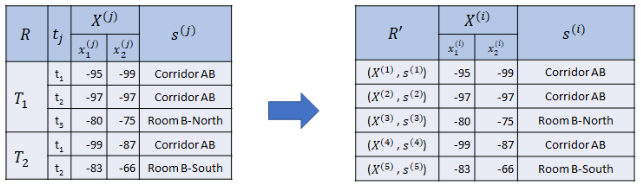
Example 3. In Figure 3, we collect two sequences of RSSI observations with semantic position and using two beacons as reference set R, where consists of three RSSI vectors and consists of two RSSI vectors. Then, we drop the sequential relationship, symbolized by the timestamp and sequence . Hence, we acquire , where , as the nonsequential reference set. Therefore, given R or , we can train the indoor positioning model for a classification with the target semantic position and input RSSI vectors . Hence, we can predict a sequence of semantic positions from an unlabeled sequence of RSSI vectors .
3.3. Indoor Semantic Trajectory
Given an indoor environment, simply represented by an indoor map, a user manually segments the whole indoor area into a set of nonoverlapping areas in terms of contextual and geographical information.
An indoor floor map contains contextual and geographical information of the indoor space. The geographical information of the indoor space includes several features such as building and room shapes, positions, surroundings, and obstructing objects (walls or any separator). Thus, we can extract the possibility (or impossibility) to reach a place from a nearby place directly. In contrast, the context gives us the semantic meaning of the areas in the indoor space, such as toilet, corridor, resting area, and exhibition area. If we combine these information, we can define the desired nonoverlapping areas in the indoor space. Each nonoverlapping area denotes a semantic position.
A person who is aware of the indoor space and its details, such as a museum manager, can define the semantic positions. In future usage, we can analyze important patterns that represent visitor behavior in the indoor space from the visited semantic positions.
With this notation, we define a semantic trajectory and movement as follows.
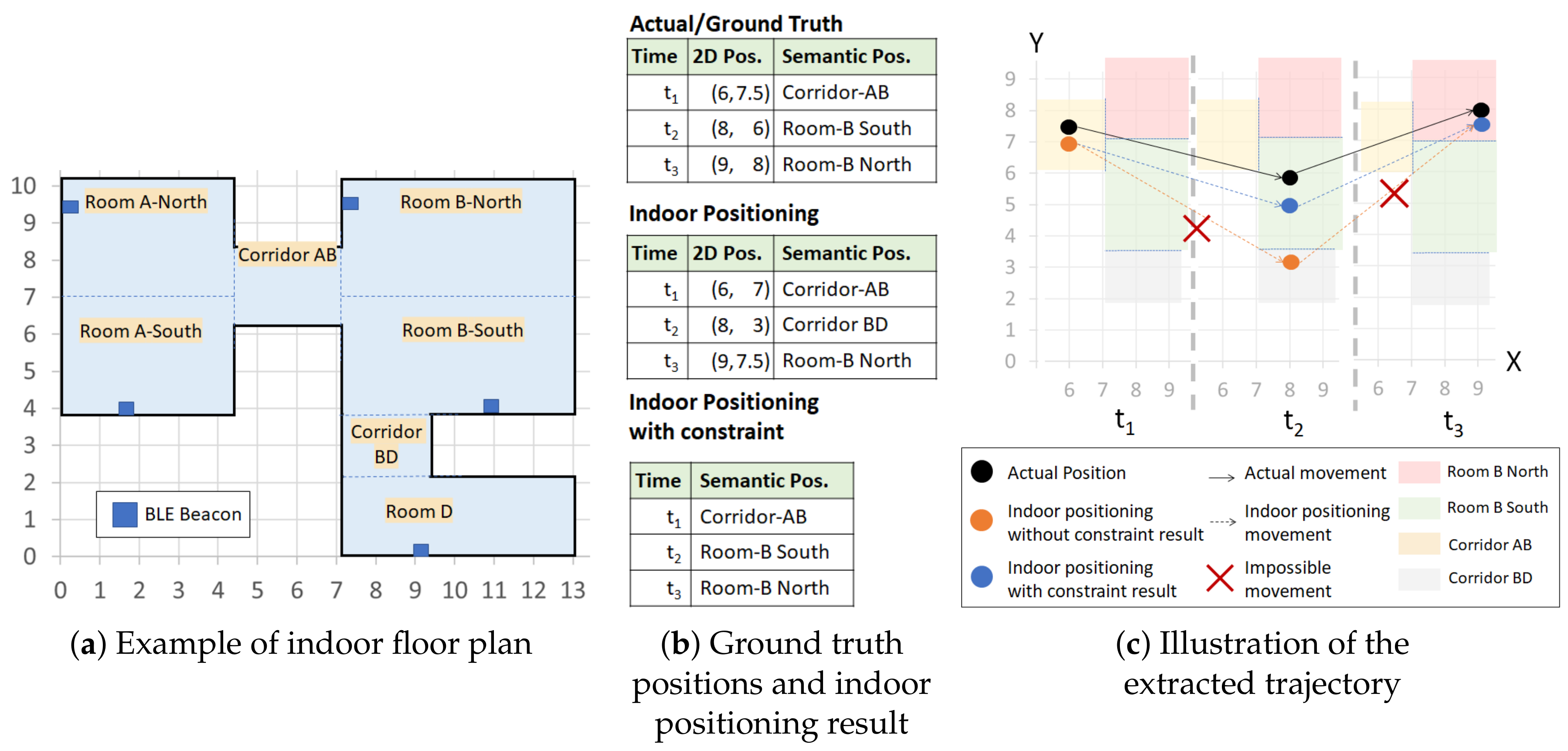
Example 4. According to the contextual and geographical meaning (area names) of the floor map in Figure 1, there are seven different semantic positions. Thus, Room A-North, Room A-South, Corridor AB, Room B-North, Room B-South, Corridor BD, Room D }. We separate Rooms A and B into northern and southern parts because each room has a large area to cover even though they are not obstructed by any object or wall. The separation is actually useful for Room B because it is impossible to reach corridor BD from northern part of Room B directly.
Definition 6. The semantic trajectory of a moving user is a sequence of timestamped semantic positions , where when and an element describes a user to be at a semantic position at time .
Definition 7. Given a semantic trajectory , we define a movement , where , as a displacement of a user from a semantic position to in a consecutive timestamp .
Example 5. A visitor in a museum walks in a similar fashion-like ground truth in Figure 1b. Thus, the visitor has a semantic trajectory ST=. We can also extract his/her movements from the semantic trajectory ST, which are and . Then, we introduce the concept of movement constraints by considering the set of neighboring semantic positiosn of a semantic position , the set of movement constraints , and the semantic graph .
Definition 8. We can define a neighbor of a semantic position if and only if there is a pair of semantic positions , where a semantic position is adjacent to and not obstructed by objects such as walls or furnitures. The neighboring semantic positions have the property of symmetry. Note that i and j are not necessarily inequal.
Definition 9. Given a semantic position , the set of neighboring semantic positions of , defined as , is a set of semantic positions where all semantic positions and the pair hold the relationship of neighboring semantic positions.
Definition 10. Given a semantic position and its neighboring set , the set of movement constraints of , defined as , consists of all possible movements from to . The movement constraint for the reverse direction also holds true as always includes (symmetric).
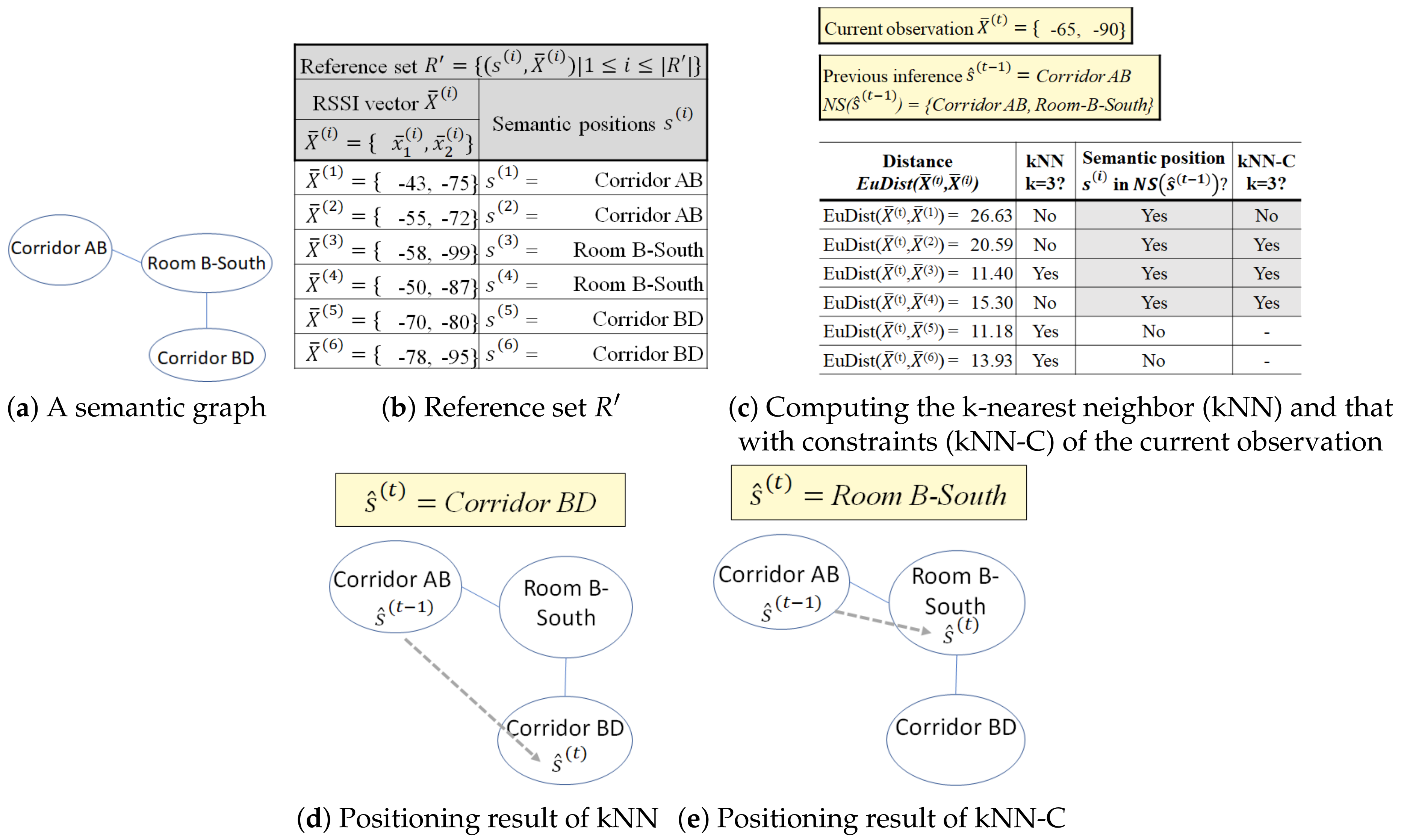
Example 6. In Figure 1, the semantic position Corridor AB has a set of neighboring semantic positions The indoor positioning technique without constraint infers as the next position at from the position at . However, to access the semantic position Corridor BD from Corridor AB, a user must visit Room B-South first. Thus, Corridor BD is not in the set of neighboring semantic positions of Corridor AB and the movement violates the movement constraint of Corridor AB, which was formally defined as and , respectively.
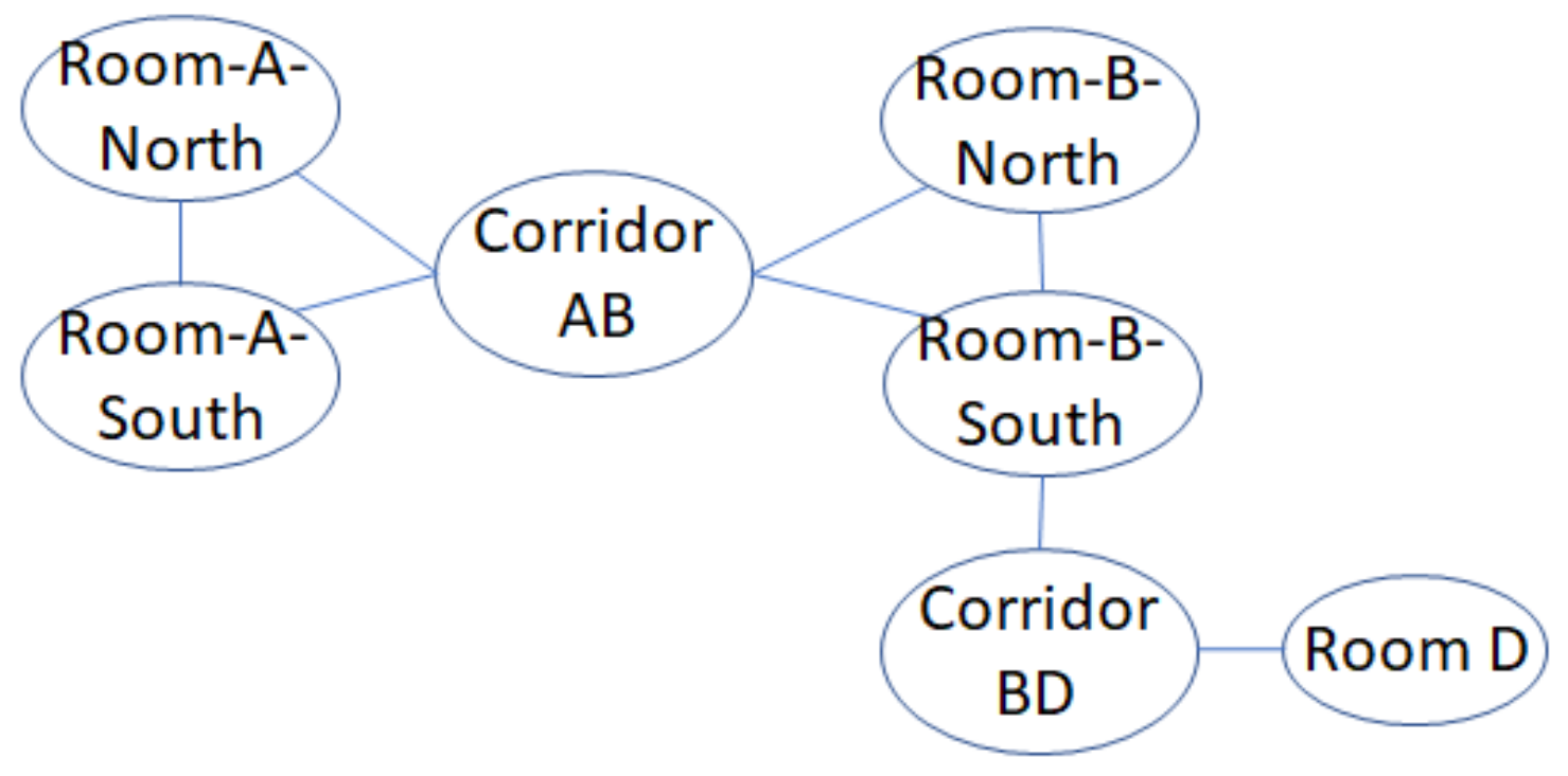
Definition 11. A semantic graph consists of a tuple , where S is a set of semantic positions and E is a set of movement constraints of all semantic positions in S. A semantic position and a set of movement constraints in semantic graph represent a vertex and the undirected edges from the respective vertex in a graph, respectively. Although they have directional properties, the movement constraints are simplified as undirected edges as they hold the symmetric relationship and .
Example 7. Semantic graph representation of the floormap in Figure 1 is depicted in Figure 4. We draw each semantic position in S as vertices. Then, for each vertex , we establish movement constraints to its neighboring semantic position set as undirected edges. If a movement constraint already exists from to (), the movement constraint from to should not be drawn. Then, we define the invalid trajectory and, consequently, the valid trajectory.
Definition 12. A semantic trajectory is an invalid trajectory that contains at least a movement that violates the movement constraint of in semantic graph such that exists.
Definition 13. A semantic trajectory is a valid trajectory when all of its movements , always complies in any movement constraint of in the semantic graph such that .
Example 8. In Figure 1c, we see an actual semantic trajectory and an estimated semantic trajectory from an indoor positioning technique (without constraint). The actual semantic trajectory is a valid trajectory as all of its movements { Corridor AB → Room B-South, Room B-South→ Room B-North} do not violate any movement constraint of {} respectively. The estimated semantic trajectory is an invalid trajectory as its two movements {Corridor AB → Corridor BD, Corridor BD → Room B-North} violate the movement constraints of {} respectively. Then, we continue to define the semantic trajectory extraction using the previously mentioned notions.
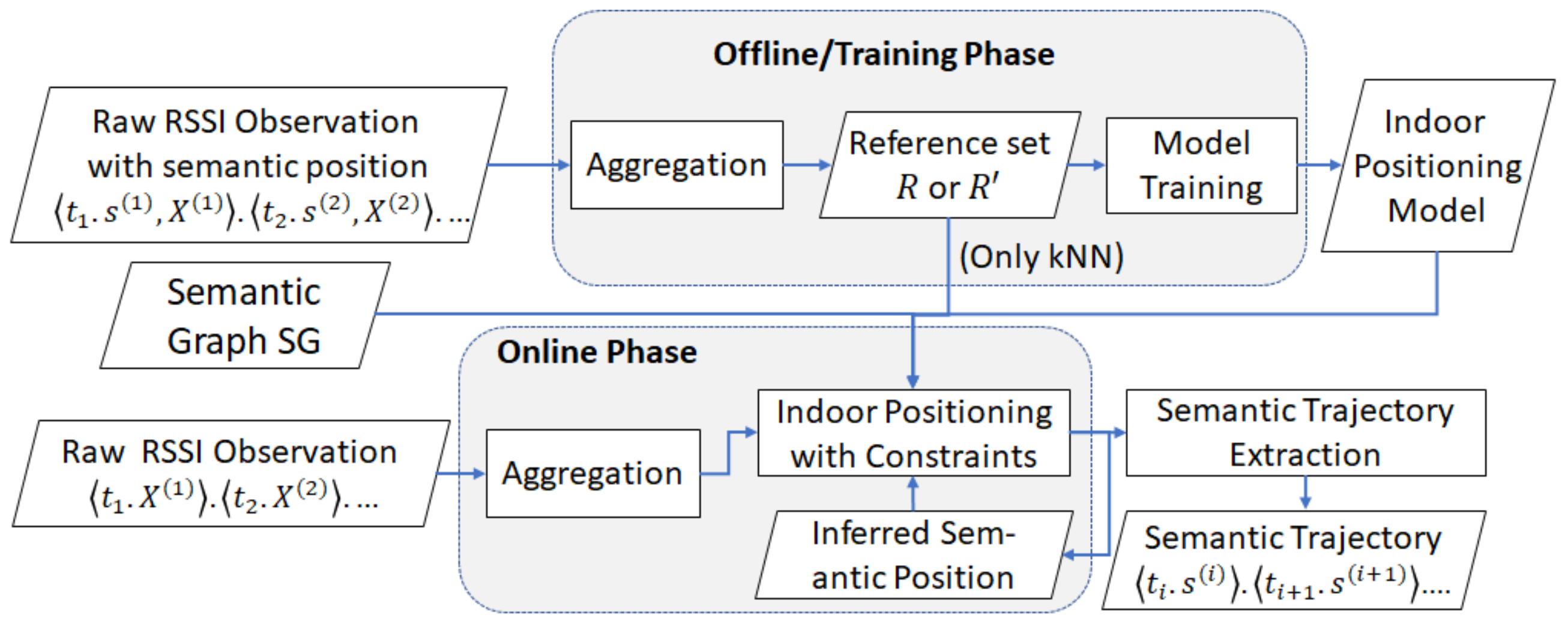
Definition 14. Semantic trajectory extraction. Given a timestamped sequence of RSSI vector and a trained indoor positioning model f with a reference set R or as training set, we estimate a semantic trajectory where each predicted semantic position corresponds to the indoor positioning function and .


