One-Shot Learning for Partial Discharge Diagnosis Using Ultra-High-Frequency Sensor in Gas-Insulated Switchgear

 ,
,
Abstract
1. Introduction
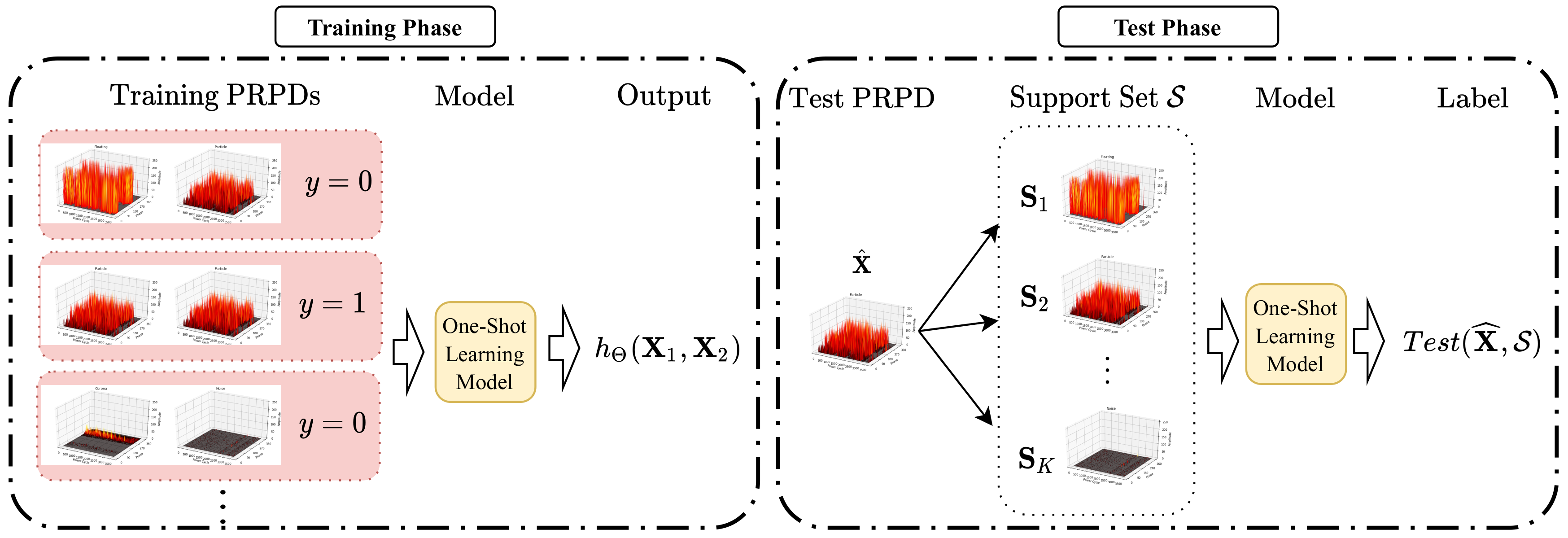
- One-shot learning is introduced for the first time to classify the PRPDs in a GIS. This method offers the advantages of a high classification accuracy while requiring a small amount of data compared with a linear SVM and CNN [30]. The proposed model uses pairs of samples of the same class or different classes during the training phase and recognizes the test sample with a single training sample for each class.
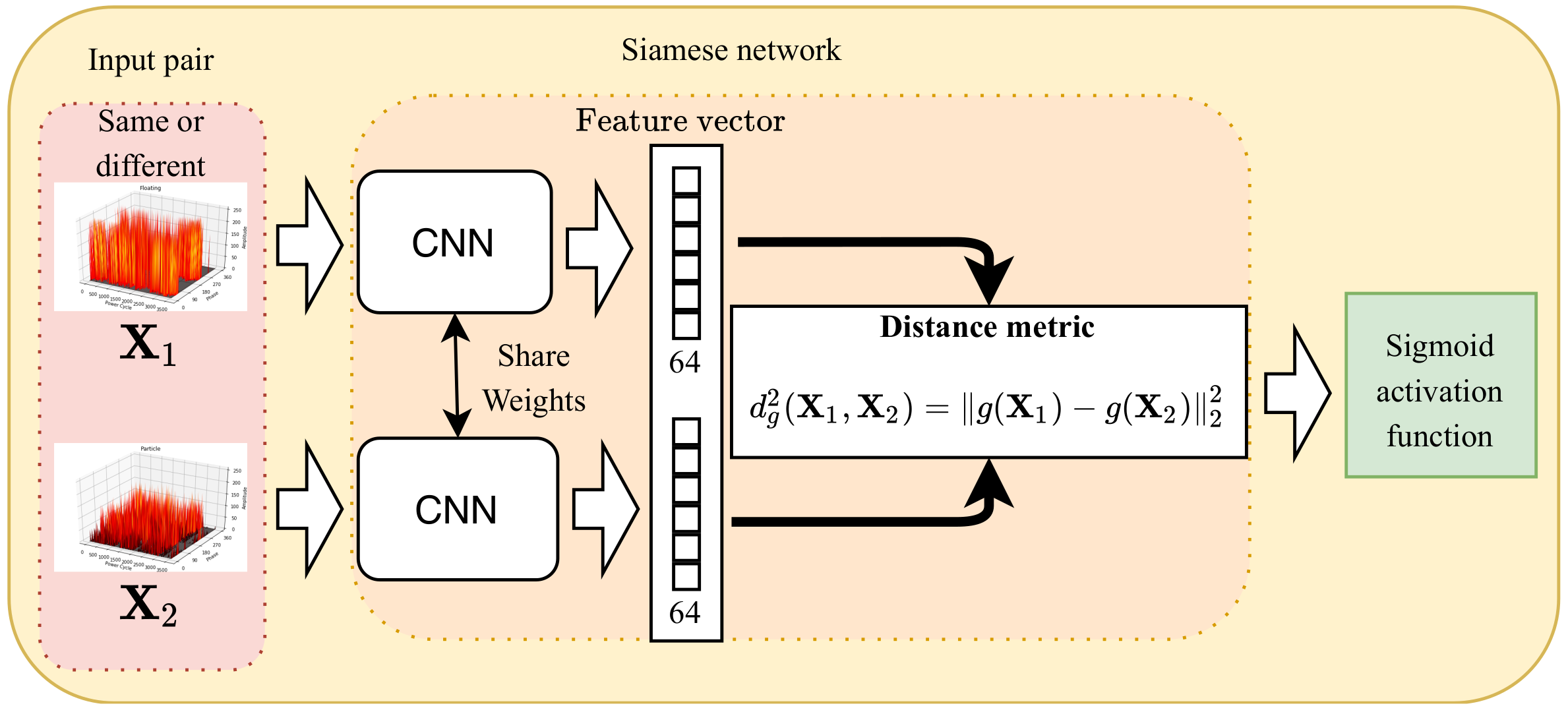
- The proposed model uses a distance metric function to map the PRPDs into a suitable embedding space and predicts the test PRPD class conditioned on the distance, which improves the classification performance as compared with that of the CNN [30].
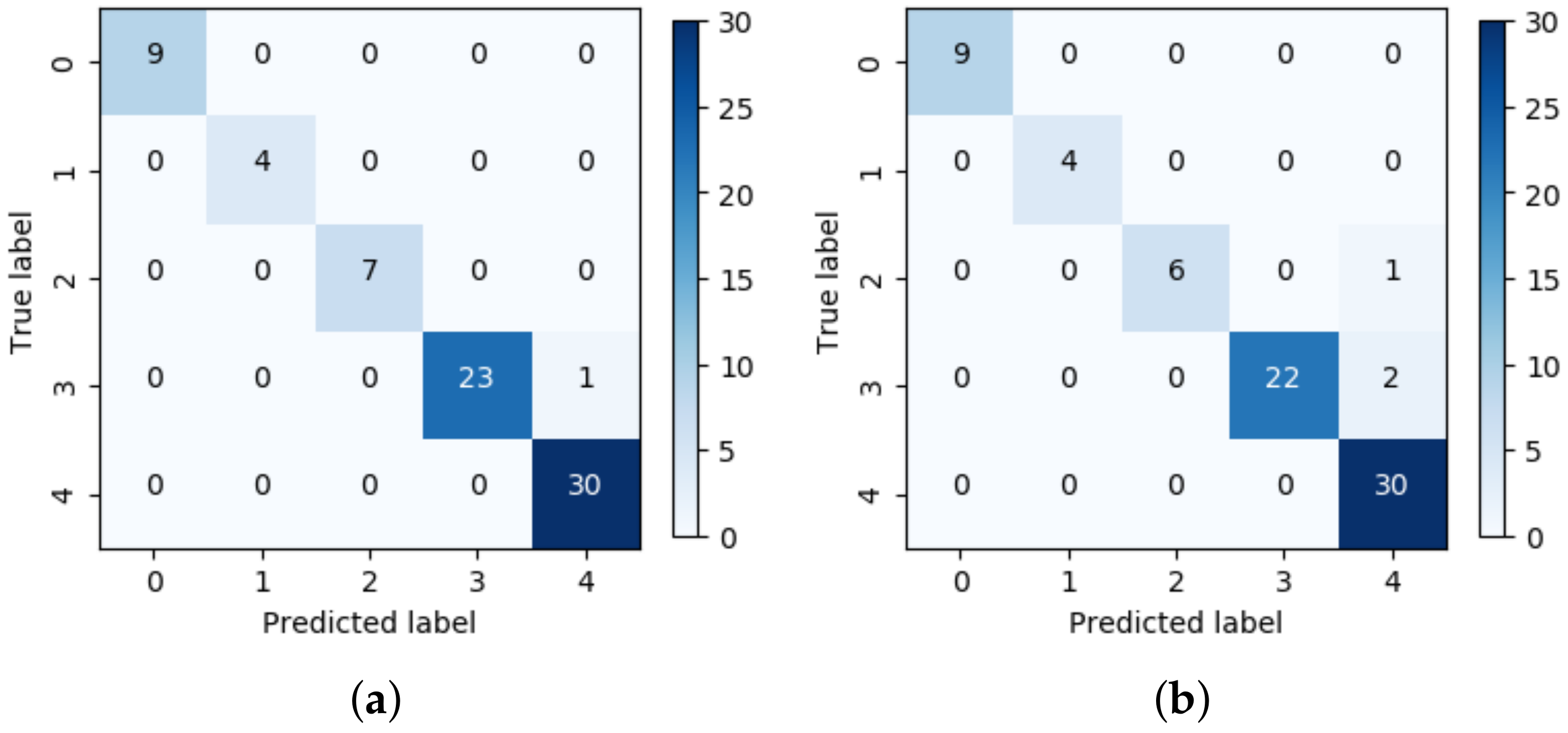
- The proposed model is verified through PRPD and on-site noise measurements using a UHF sensor. The proposed model achieves a classification accuracy of 98.65% for four types of faults and noise in the GIS.
2. Prpd and Noise Measurements
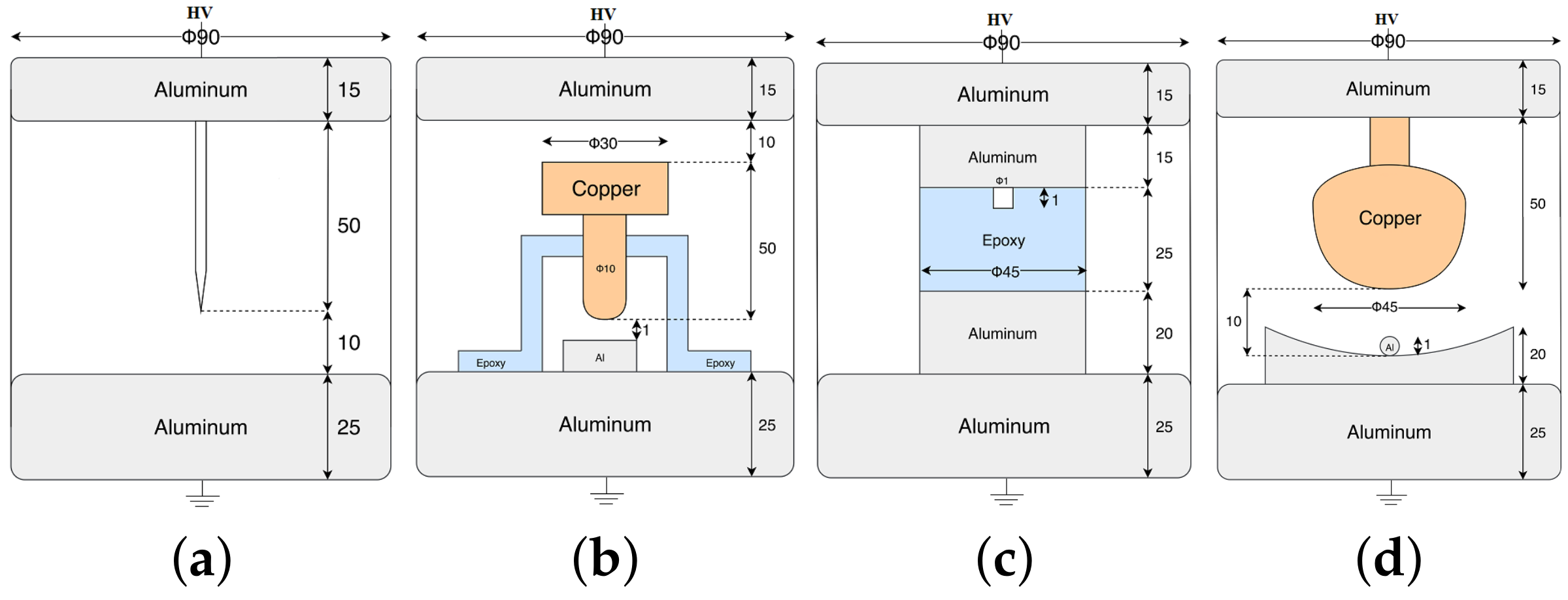
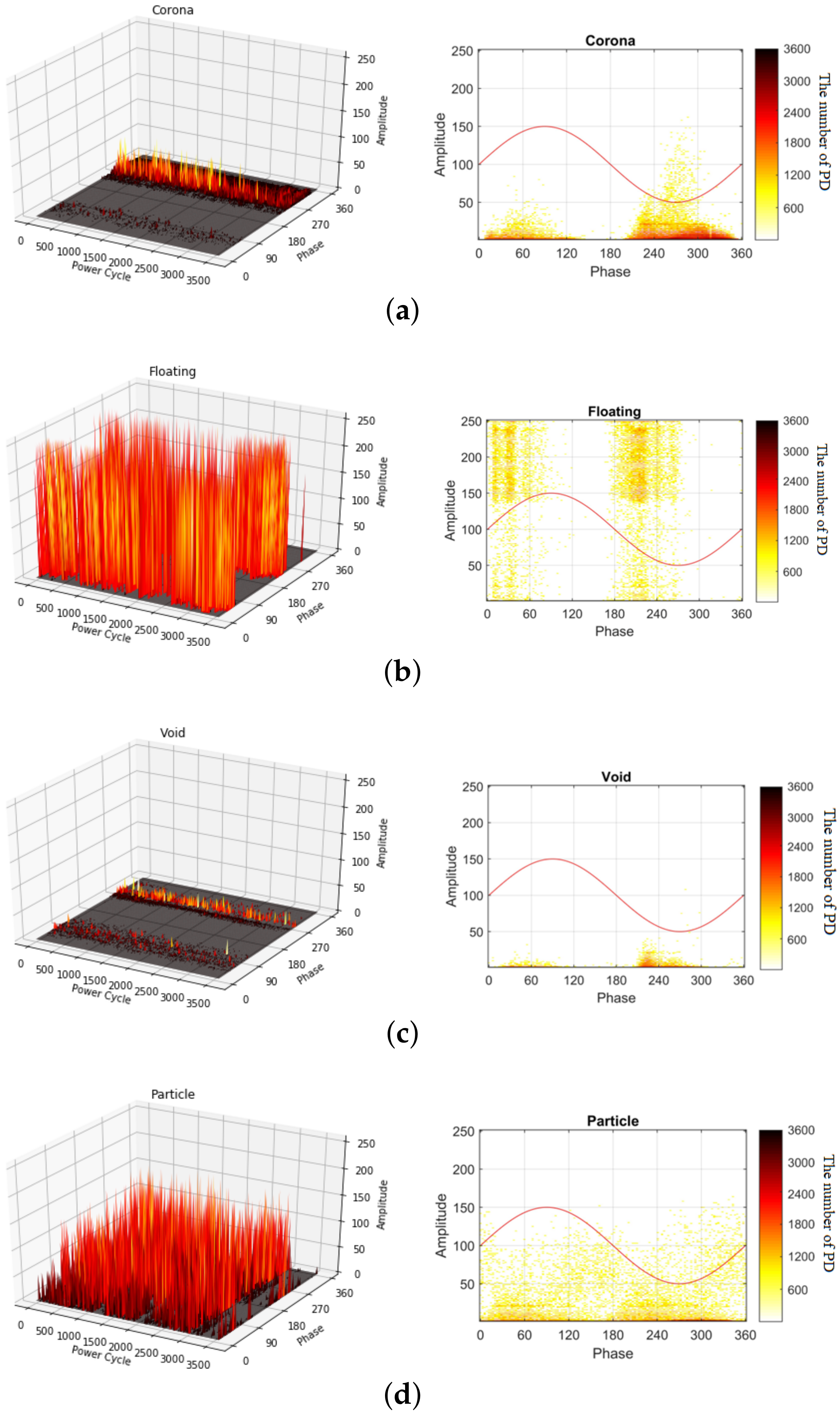
2.1. Prpd Measurements in Gis
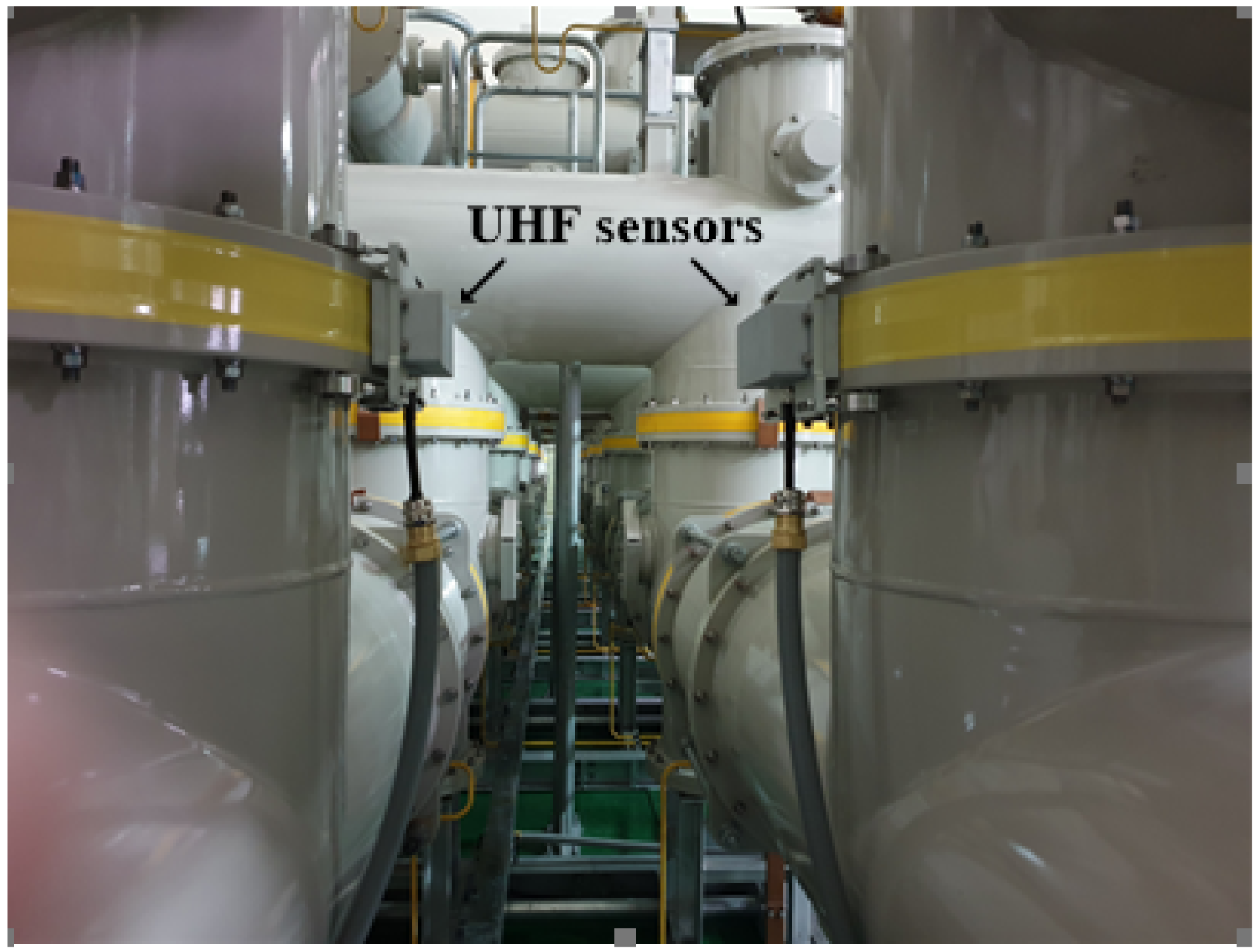
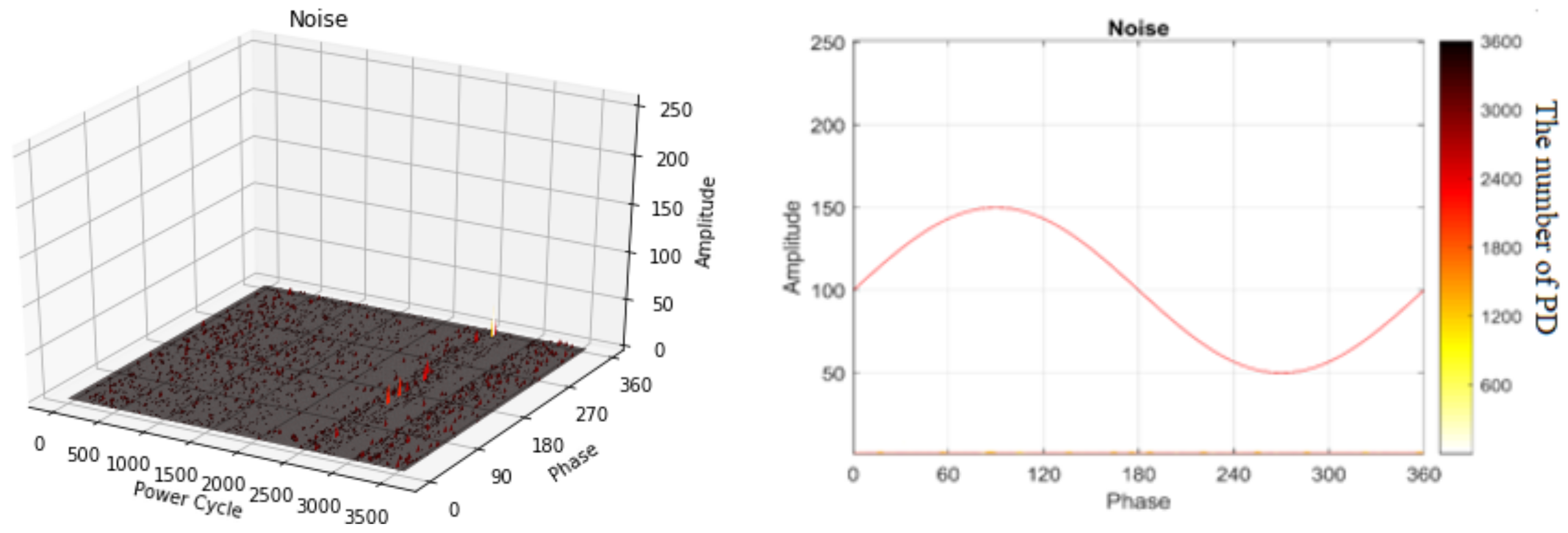
2.2. On-Site Noise Measurements
3. Proposed Method
3.1. One-Shot Learning Model
3.2. Network Optimization
4. Experiment Results
5. Conclusions
Author Contributions
Funding
Conflicts of Interest
References
- Riera-Guasp, M.; Antonino-Daviu, J.A.; Capolino, G.-A. Advances in Electrical Machine, Power Electronic, and Drive Condition Monitoring and Fault Detection: State of the Art. IEEE Trans. Ind. Electron. 2015, 62, 1746–1759. [Google Scholar] [CrossRef]
- Lu, C.; Wenrong, S.; Chenzhao, F.; Kai, G. The Development of UHF Sensor for GIS Partial Discharge Measurement. In Proceedings of the 2019 IEEE 2nd International Conference on Automation, Electronics and Electrical Engineering (AUTEEE), Shenyang, China, 22–24 November 2019; pp. 287–290. [Google Scholar]
- Rao, M.M.; Kumar, M. Ultra-High Frequency (UHF) Based Partial Discharge Measurement in Gas Insulated Switchgear (GIS). In Proceedings of the 2019 IEEE International Conference on High Voltage Engineering and Technology (ICHVET), Hyderabad, India, 7–8 February 2019; pp. 1–5. [Google Scholar]
- Phung, B.T.; Blackburn, T.R.; Liu, Z. Acoustic measurements of partial discharge signals. J. Electr. Electron. Eng. Aust. 2001, 21, 41. [Google Scholar]
- Descoeudres, A.; Hollenstein, C.; Demellayer, R.; Wälder, G. Optical emission spectroscopy of electrical discharge machining plasma. J. Mater. Process. Technol. 2004, 149, 184–190. [Google Scholar] [CrossRef]
- Biswas, S.; Koley, C.; Chatterjee, B.; Chakravorti, S. A methodology for identification and localization of partial discharge sources using optical sensors. IEEE Trans. Dielectr. Electr. Insul. 2012, 19, 18–28. [Google Scholar] [CrossRef]
- Duval, M. A review of faults detectable by gas-in-oil analysis in transformers. IEEE Electr. Insul. Mag. 2002, 18, 8–17. [Google Scholar] [CrossRef]
- Han, X.; Li, J.; Zhang, L.; Pang, P.; Shen, S. A Novel PD Detection Technique for Use in GIS Based on a Combination of UHF and Optical Sensors. IEEE Trans. Instrum. Meas. 2019, 68, 2890–2897. [Google Scholar] [CrossRef]
- IEC-62478. High-Voltage Test Techniques—Measurement of Partial Discharges by Electromagnetic and Acoustic Methods. Proposed Horizontal Standard, 1st ed.; International Electrotechnical Commission (IEC): Geneva, Switzerland, 2016. [Google Scholar]
- Hoshino, T.; Koyama, H.; Maruyama, S.; Hanai, M. Comparison of sensitivity between UHF method and IEC 60270 for onsite calibration in various GIS. IEEE Trans. Power Deliv. 2006, 21, 1948–1953. [Google Scholar] [CrossRef]
- Tenbohlen, S.; Denissov, D.; Hoek, S.; Markalous, S.M. Partial discharge measurement in the ultra high frequency (UHF) range. IEEE Trans. Dielectr. Electr. Insul. 2008, 15, 1544–1552. [Google Scholar] [CrossRef]
- Suprianto, I.; Khayam, U.; Nishigouchi, K.; Kamarol, M.; Kozako, M.; Hikita, M. UHF sensor optimization used for detecting partial discharge emitted electromagnetic wave in gas insulated switchgear. In Proceedings of the 2014 IEEE International Symposium on Electrical Insulating Materials, Niigata, Japan, 1–5 June 2014; pp. 229–232. [Google Scholar]
- Raymond, W.J.K.; Illias, H.A.; Bakar, A.H.A.; Mokhlis, H. Partial discharge classifications: Review of recent progress. Measurement 2015, 68, 164–181. [Google Scholar] [CrossRef]
- Mor, A.R.; Heredia, L.C.C.; Munoz, F.A. Estimation of charge, energy and polarity of noisy partial discharge pulses. IEEE Trans. Dielect. Electr. Insul. 2017, 24, 2511–2521. [Google Scholar] [CrossRef]
- Mor, A.R.; Morshuis, P.H.F.; Smit, J.J. Comparison of charge estimation methods in partial discharge cable measurements. IEEE Trans. Dielect. Electr. Insul. 2015, 22, 657–664. [Google Scholar] [CrossRef]
- Nair, R.P.; Vishwanath, S.B. Analysis of partial discharge sources in stator insulation system using variable excitation frequency. IET Sci. Meas. Technol. 2019, 13, 922–930. [Google Scholar] [CrossRef]
- Chen, X.; Qian, Y.; Sheng, G.; Jiang, X. A time-domain characterization method for UHF partial discharge sensors. IEEE Trans. Dielect. Electr. Insul. 2017, 24, 110–119. [Google Scholar] [CrossRef]
- Jahangir, H.; Akbari, A.; Werle, P.; Akbari, M.; Szczechowski, J. UHF characteristics of different types of PD sources in power transformers. In Proceedings of the 2017 IEEE Iranian Conference on Electrical Engineering (ICEE), Tehran, Iran, 2–4 May 2017; pp. 1242–1247. [Google Scholar]
- Sahoo, N.C.; Salama, M.M.A.; Bartnikas, R. Trends in partial discharge pattern classification: A survey. IEEE Trans. Dielect. Electr. Insul. 2005, 12, 248–264. [Google Scholar] [CrossRef]
- Karthikeyan, B.; Gopal, S.; Venkatesh, S. Partial discharge pattern classification using composite versions of probabilistic neural network inference engine. Expert Syst. Appl. 2008, 34, 1938–1947. [Google Scholar] [CrossRef]
- Umamaheswari, R.; Sarathi, R. Identification of Partial Discharges in Gas-insulated Switchgear by Ultra-high-frequency Technique and Classification by Adopting Multi-class Support Vector Machines. Electr. Power Components Syst. 2011, 39, 1577–1595. [Google Scholar] [CrossRef]
- Abdel-Galil, T.; Sharkawy, R.; Salama, M.; Bartnikas, R. Partial Discharge Pattern Classification Using the Fuzzy Decision Tree Approach. IEEE Trans. Instrum. Meas. 2005, 54, 2258–2263. [Google Scholar] [CrossRef]
- Darabad, V.P.; Vakilian, M.; Blackburn, T.R.; Phung, B.T. An efficient PD data mining method for power transformer defect models using SOM technique. Int. J. Electr. Power Energy Syst. 2015, 71, 373–382. [Google Scholar] [CrossRef]
- Abubakar Mas’ud, A.; Stewart, B.G.; McMeekin, S.G. Application of an ensemble neural network for classifying partial discharge patterns. Electr. Power Syst. Res. 2014, 110, 154–162. [Google Scholar] [CrossRef]
- LeCun, Y.; Bengio, Y.; Hinton, G. Deep learning. Nature 2015, 521, 436–444. [Google Scholar] [CrossRef]
- Li, G.; Wang, X.; Li, X.; Yang, A.; Rong, M. Partial Discharge Recognition with a Multi-Resolution Convolutional Neural Network. Sensors 2018, 18, 3512. [Google Scholar] [CrossRef] [PubMed]
- Nguyen, M.T.; Nguyen, V.H.; Yun, S.J.; Kim, Y.H. Recurrent Neural Network for Partial Discharge Diagnosis in Gas-Insulated Switchgear. Energies 2018, 11, 1202. [Google Scholar] [CrossRef]
- Tuyet-Doan, V.-N.; Nguyen, T.-T.; Nguyen, M.-T.; Lee, J.-H.; Kim, Y.-H. Self-Attention Network for Partial-Discharge Diagnosis in Gas-Insulated Switchgear. Energies 2020, 13, 2102. [Google Scholar] [CrossRef]
- Hsiao, S.-C.; Kao, D.-Y.; Liu, Z.-Y.; Tso, R. Malware Image Classification Using One-Shot Learning with Siamese Networks. Procedia Comput. Sci. 2019, 159, 1863–1871. [Google Scholar] [CrossRef]
- Zhang, A.; Li, S.; Cui, Y.; Yang, W.; Dong, R.; Hu, J. Limited Data Rolling Bearing Fault Diagnosis with Few-Shot Learning. IEEE Access 2019, 7, 110895–110904. [Google Scholar] [CrossRef]
- Koch, G.; Zemel, R.; Salakhutdinov, R. Siamese neural networks for one-shot image recognition. In Proceedings of the 2nd ICML Deep Learning Workshop, Lille, France, 10–11 July 2015. [Google Scholar]
- Vedral, J.; Kříž, M. Signal Processing in Partial Discharge Measurement. Metrol. Meas. Syst. 2010, 17, 55–64. [Google Scholar] [CrossRef][Green Version]
- Wang, B.; Wang, D. Plant Leaves Classification: A Few-Shot Learning Method Based on Siamese Network. IEEE Access 2019, 7, 151754–151763. [Google Scholar] [CrossRef]
- Nair, V.; Hinton, G.E. Rectified Linear Units Improve Restricted Boltzmann Machines. In Proceedings of the 27th International Conference on International Conference on Machine Learning (ICML’10), Haifa, Israel, 21–24 June 2010; Volume 27, pp. 807–814. [Google Scholar]
- Srivastava, N.; Hinton, G.; Krizhevsky, A.; Sutskever, I.; Salakhutdinov, R. Dropout: A simple way to prevent neural networks from overfitting. J. Mach. Learn. Res. 2014, 15, 1929–1958. [Google Scholar]
- Ioffe, S.; Szegedy, C. Batch Normalization: Accelerating Deep Network Training by Reducing Internal Covariate Shift. In Proceedings of the 32nd International Conference on Machine Learning, Lille, France, 6–11 July 2015; pp. 448–456. [Google Scholar]
- Duchi, J.; Hazan, E.; Singer, Y. Adaptive Subgradient Methods for Online Learning and Stochastic Optimization. J. Mach. Learn. Res. 2011, 12, 2121–2159. [Google Scholar]
- Zeiler, M.D. ADADELTA: An Adaptive Learning Rate Method. arXiv 2012, arXiv:1212.5701. [Google Scholar]
- Dozat, T. Incorporating Nesterov Momentum into Adam. In Proceedings of the ICLR Workshop, Caribe Hilton, San Juan, Puerto Rico, 2–4 May 2016; pp. 2013–2016. [Google Scholar]
- Kingma, D.P.; Ba, J. Adam: A Method for Stochastic Optimization. In Proceedings of the 3rd International Conference for Learning Representations, San Diego, CA, USA, 7–9 May 2015; pp. 807–814. [Google Scholar]
- Abadi, M.; Agarwal, A.; Barham, P.; Brevdo, E.; Chen, Z.; Citro, C.; Corrado, G.; Davis, A.; Dean, J.; Devin, M. TensorFlow: Large-Scale Machine Learning on Heterogeneous Distributed Systems. 2015. Available online: https://www.tensorflow.org/ (accessed on 8 June 2020).
- Keras-Team. 2015. Available online: https://github.com/fchollet/keras (accessed on 8 June 2020).


| Fault Types | Corona | Floating | Particle | Void | Noise |
|---|---|---|---|---|---|
| (0) | (1) | (2) | (3) | (4) | |
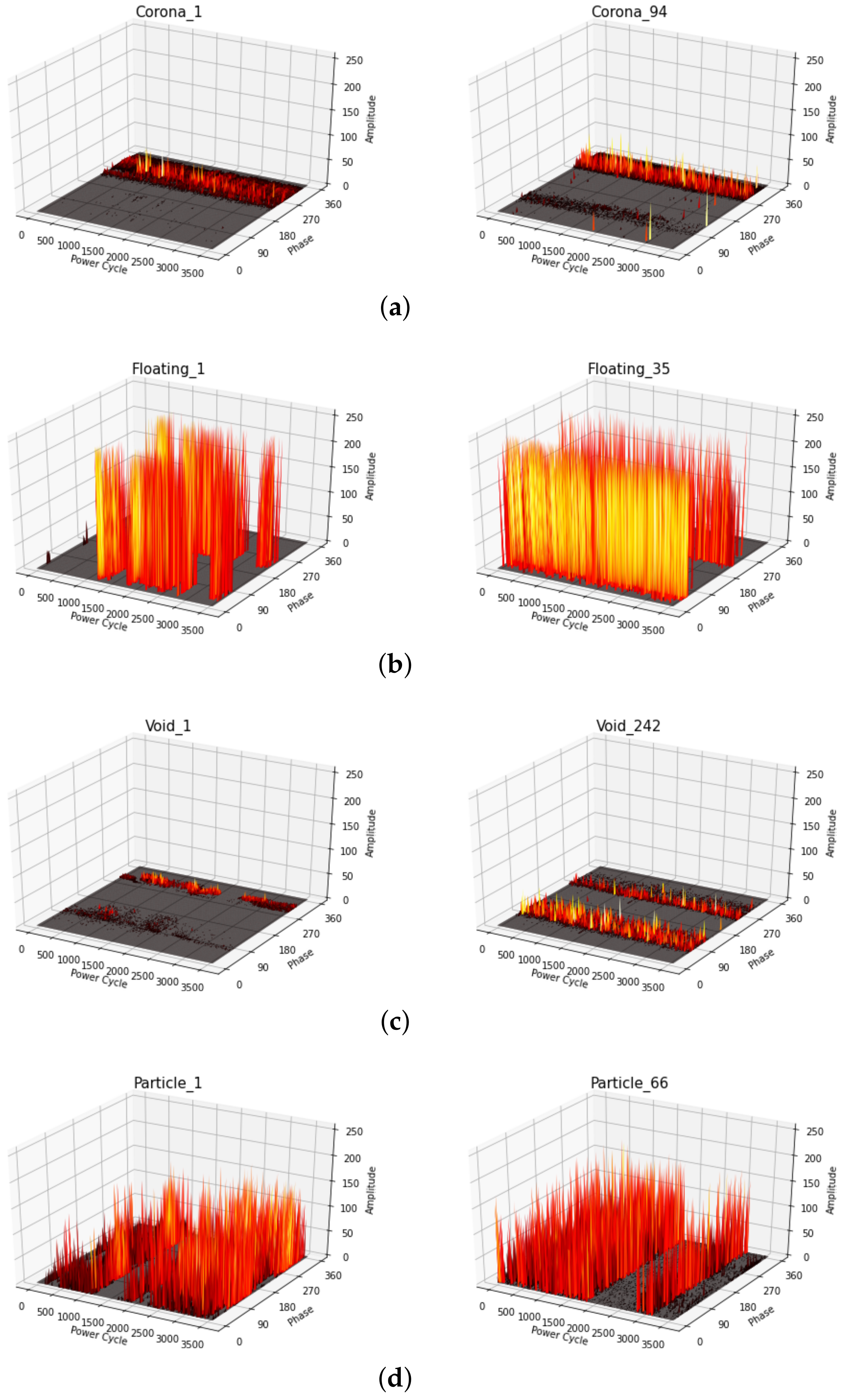
| Number of experiments | 94 | 35 | 66 | 242 | 298 |
| Kernel | Kernel | ||||
|---|---|---|---|---|---|
| No. | Layer Type | Size/Stride | Number | Output Size | Padding |
| 1 | Convolution 1 | 16 × 16/4 | 16 | 900 × 32 × 16 | same |
| 2 | Max-Pooling 1 | 2 × 2/2 | - | 450 × 16 × 16 | valid |
| 3 | Batch Normalization 1 | - | - | 450 × 16 × 16 | - |
| 4 | Drop Out 1 | - | - | 450 × 16 × 16 | - |
| 5 | Convolution 2 | 3 × 3/1 | 32 | 450 × 16 × 32 | same |
| 6 | Max-Pooling 2 | 2 × 2/2 | - | 225 × 8 × 32 | valid |
| 7 | Batch Normalization 2 | - | - | 225 × 8 × 32 | - |
| 8 | Drop Out 2 | - | - | 225 × 8 × 32 | - |
| 9 | Convolution 3 | 3 × 3/1 | 64 | 225 × 8 × 64 | same |
| 10 | Max-Pooling 3 | 2 × 2/2 | - | 112 × 4 × 64 | valid |
| 11 | Batch Normalization 3 | - | - | 112 × 4 × 64 | - |
| 12 | Drop Out 3 | - | - | 112 × 4 × 64 | - |
| 13 | Convolution 4 | 3 × 3/1 | 64 | 112 × 4 × 64 | same |
| 14 | Max-Pooling 4 | 2 × 2/2 | - | 56 × 2 × 64 | valid |
| 15 | Batch Normalization 4 | - | - | 56 × 2 × 64 | - |
| 16 | Drop Out 4 | - | - | 56 × 2 × 64 | - |
| 17 | Flatten 1 | - | - | 7168 × 1 | - |
| 18 | Dense 2 | 64 | - | 64 × 1 | - |
| Fault Types | Overall | Corona | Floating | Particle | Void | Noise |
|---|---|---|---|---|---|---|
| (%) | (%) | (%) | (%) | (%) | (%) | |
| Linear SVM | 92.28 | 100 | 25 | 28.57 | 83.33 | 73.33 |
| CNN | 95.95 | 100 | 100 | 85.71 | 91.67 | 100 |
| One-shot learning | 98.65 | 100 | 100 | 100 | 95.83 | 100 |
| Fault Types | Overall | Corona | Floating | Particle | Void | Noise |
|---|---|---|---|---|---|---|
| (%) | (%) | (%) | (%) | (%) | (%) | |
| Linear SVM | 72.22 | 75 | 100 | 50 | 33.33 | 100 |
| CNN | 88.89 | 75 | 67.67 | 100 | 100 | 100 |
| One-shot learning | 94.44 | 75 | 100 | 100 | 100 | 100 |
© 2020 by the authors. Licensee MDPI, Basel, Switzerland. This article is an open access article distributed under the terms and conditions of the Creative Commons Attribution (CC BY) license (http://creativecommons.org/licenses/by/4.0/).
Share and Cite
Tuyet-Doan, V.-N.; Do, T.-D.; Tran-Thi, N.-D.; Youn, Y.-W.; Kim, Y.-H. One-Shot Learning for Partial Discharge Diagnosis Using Ultra-High-Frequency Sensor in Gas-Insulated Switchgear. Sensors 2020, 20, 5562. https://doi.org/10.3390/s20195562
Tuyet-Doan V-N, Do T-D, Tran-Thi N-D, Youn Y-W, Kim Y-H. One-Shot Learning for Partial Discharge Diagnosis Using Ultra-High-Frequency Sensor in Gas-Insulated Switchgear. Sensors. 2020; 20(19):5562. https://doi.org/10.3390/s20195562
Chicago/Turabian StyleTuyet-Doan, Vo-Nguyen, The-Duong Do, Ngoc-Diem Tran-Thi, Young-Woo Youn, and Yong-Hwa Kim. 2020. "One-Shot Learning for Partial Discharge Diagnosis Using Ultra-High-Frequency Sensor in Gas-Insulated Switchgear" Sensors 20, no. 19: 5562. https://doi.org/10.3390/s20195562
APA StyleTuyet-Doan, V.-N., Do, T.-D., Tran-Thi, N.-D., Youn, Y.-W., & Kim, Y.-H. (2020). One-Shot Learning for Partial Discharge Diagnosis Using Ultra-High-Frequency Sensor in Gas-Insulated Switchgear. Sensors, 20(19), 5562. https://doi.org/10.3390/s20195562