A Recurrent Deep Network for Estimating the Pose of Real Indoor Images from Synthetic Image Sequences


Abstract
1. Introduction
- We improve the localisation accuracy of pose regression networks that use synthetic images to estimate the camera pose of real images. The spatio-temporal constraint of image sequences is utilised to improve accuracy and to generate a smoother trajectory.
- The uncertainty of camera pose estimation is modelled by sampling from a sliding window of image sequences. We show that the modelled uncertainty shows correlation with the errors.
2. Background and Related Work
2.1. Image-Based Retrieval Approaches
2.1.1. Using Point Features
2.1.2. Depth-Based Approaches
2.1.3. CNN-Based Approaches
2.2. Use of Synthetic Images
2.3. Limitations of Current Approaches
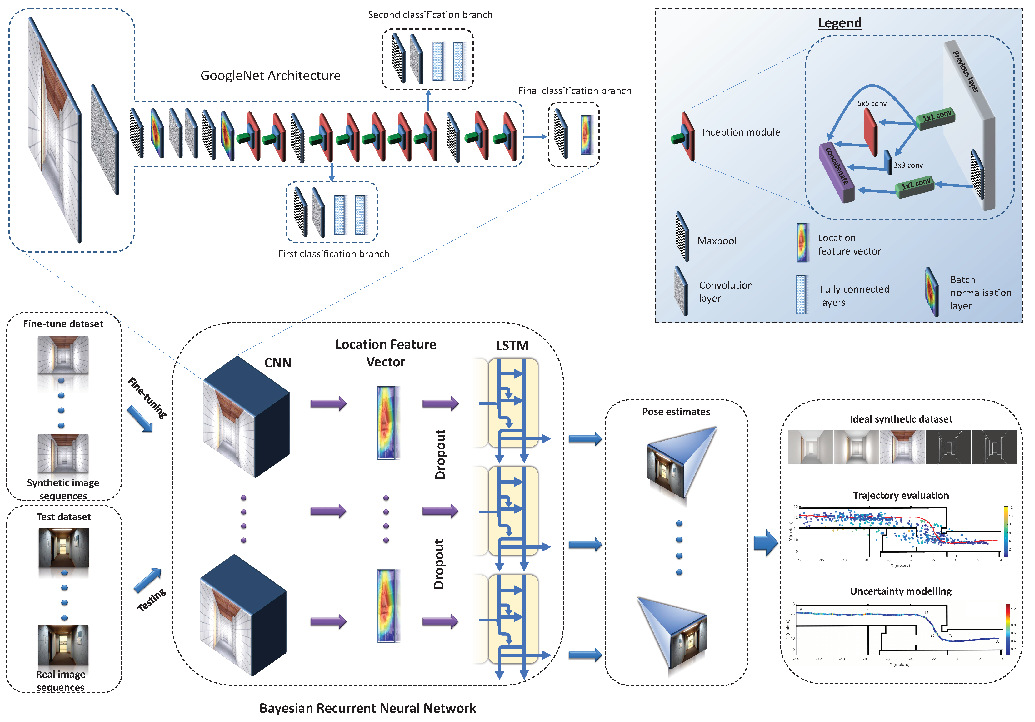
3. Methodology
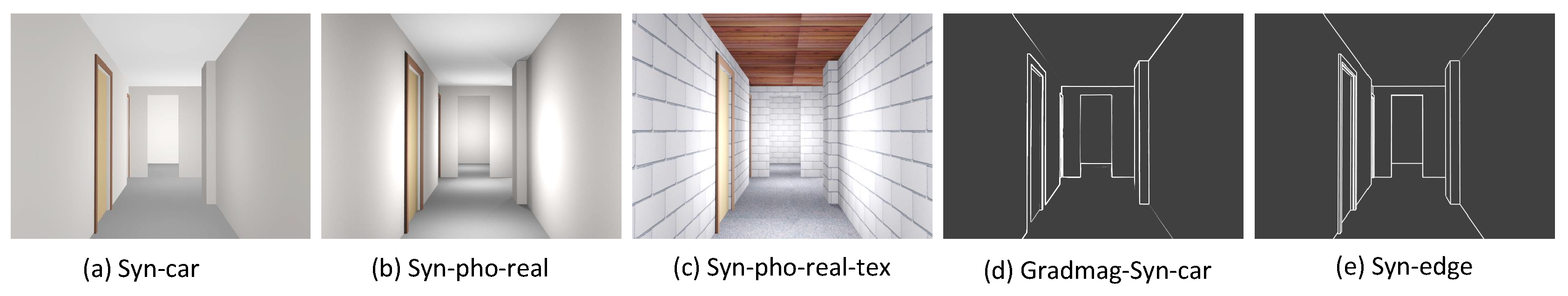
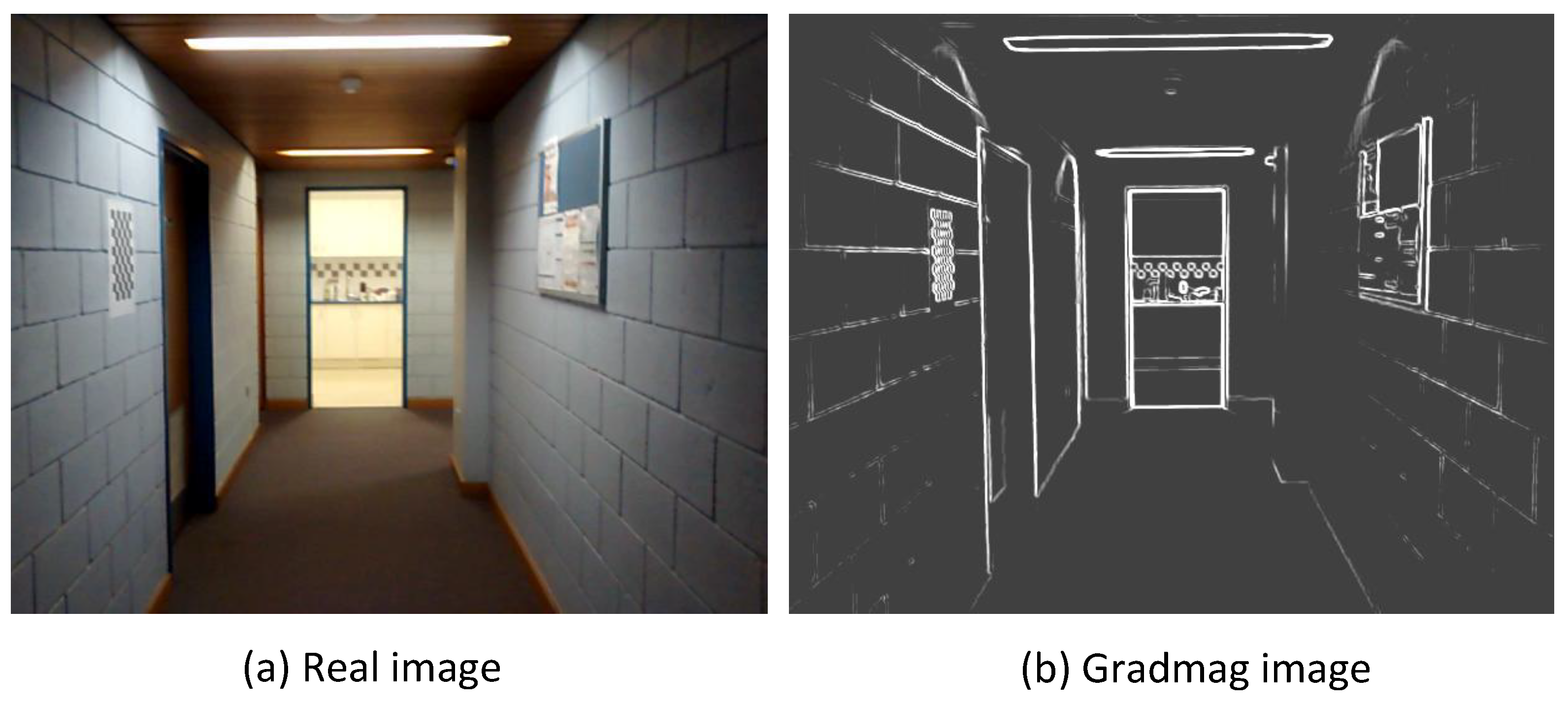
3.1. Generation of Synthetic Image Sequences
3.2. Deep Learning Architecture
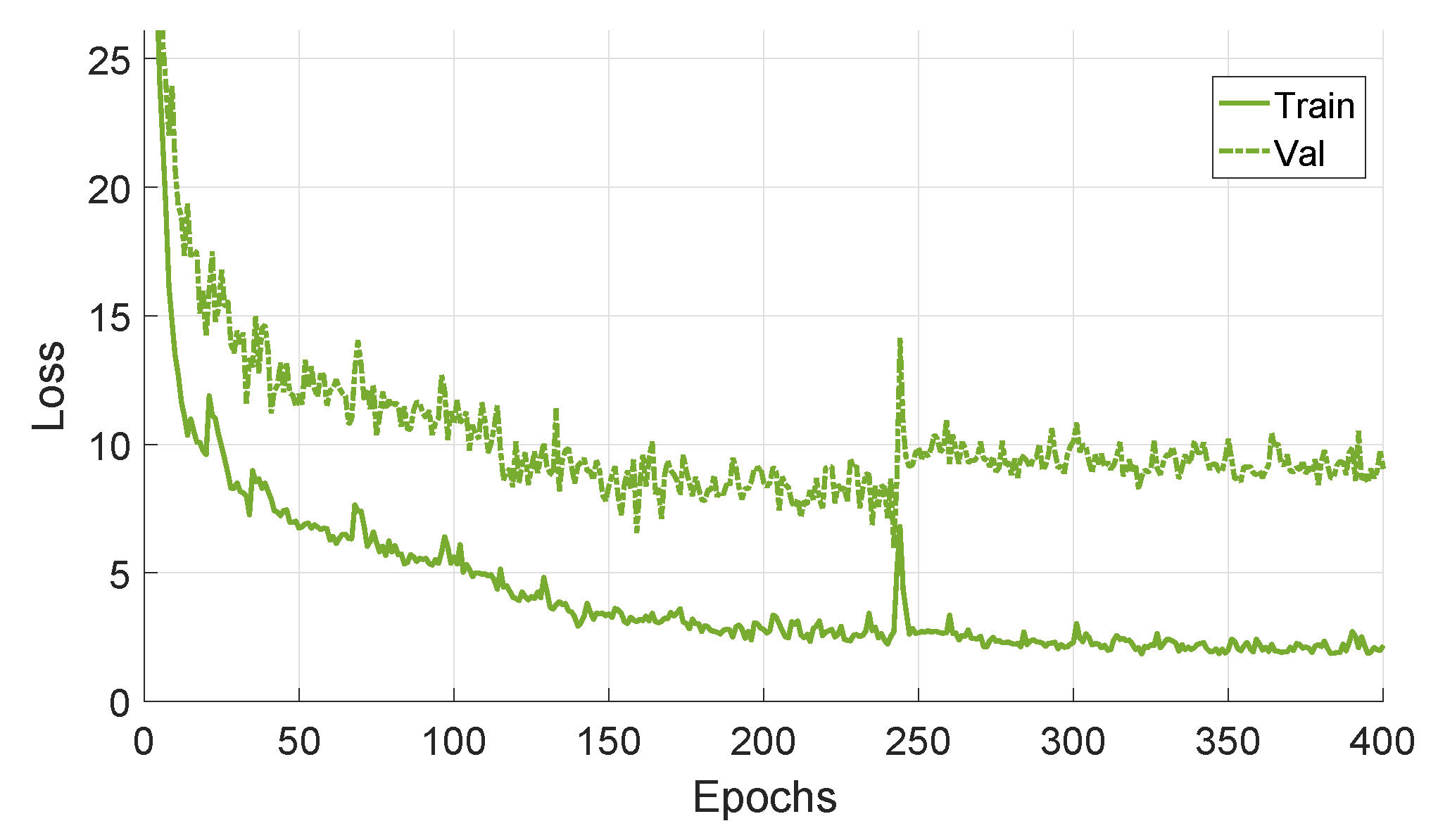
3.3. Fine-Tuning and Loss Function
3.4. Modelling Uncertainty
4. Experiments and Results
4.1. Implementation Details
4.2. Experimental Design
- Experiment 1: Using real images for training and testing. A baseline accuracy was established by fine-tuning Recurrent BIM-PoseNet using real images, to compare the results obtained from the proposed approach being fine-tuned using synthetic data. Parameters such as ideal LSTM length, ideal window length and the correlation of localisation errors with the estimated localisation uncertainties are identified. The results are presented in Section 4.4.
- Experiment 2: Using synthetic images for training and real images for testing. In this experiment, Recurrent BIM-PoseNet was fine-tuned using several types of synthetic image sequences. Subsequently, pose regression ability of these fine-tuned networks were evaluated by using real image sequences during test, and compared with the previous approaches. The results are presented in Section 4.5.
- Experiment 3: Modelling uncertainty. This experiment consisted of modelling the uncertainty of the estimated camera poses, and evaluating the correlation of the localisation errors with the estimated localisation uncertainties. The results are compared with the results of Bayesian BIM-PoseNet, and are presented in Section 4.6.
4.3. Dataset
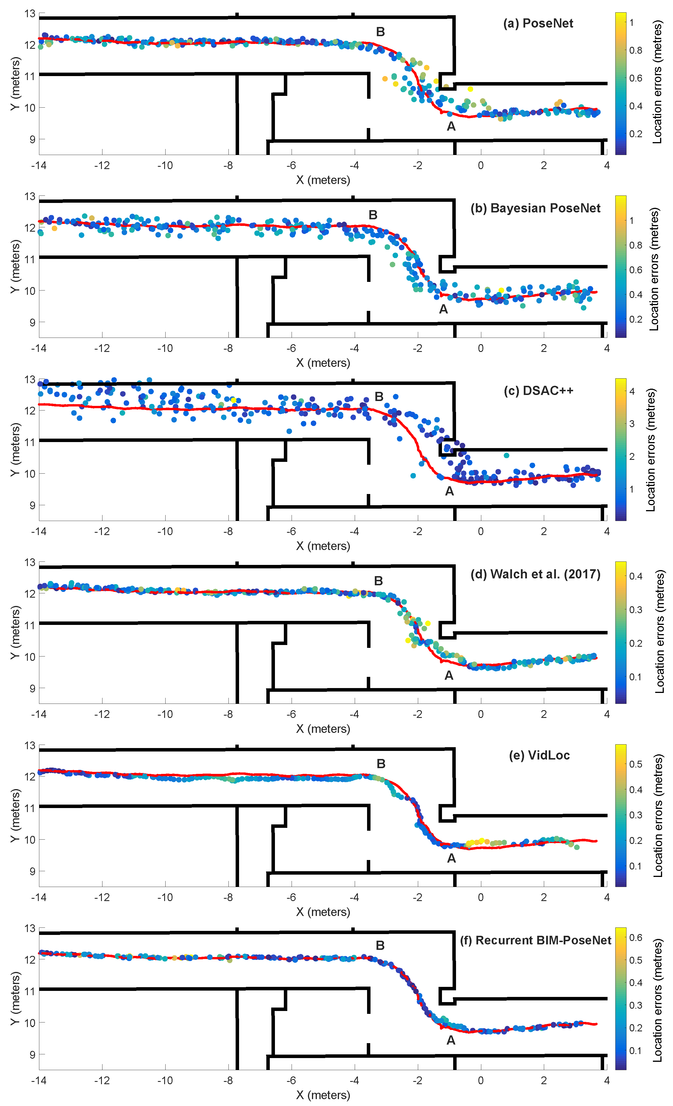
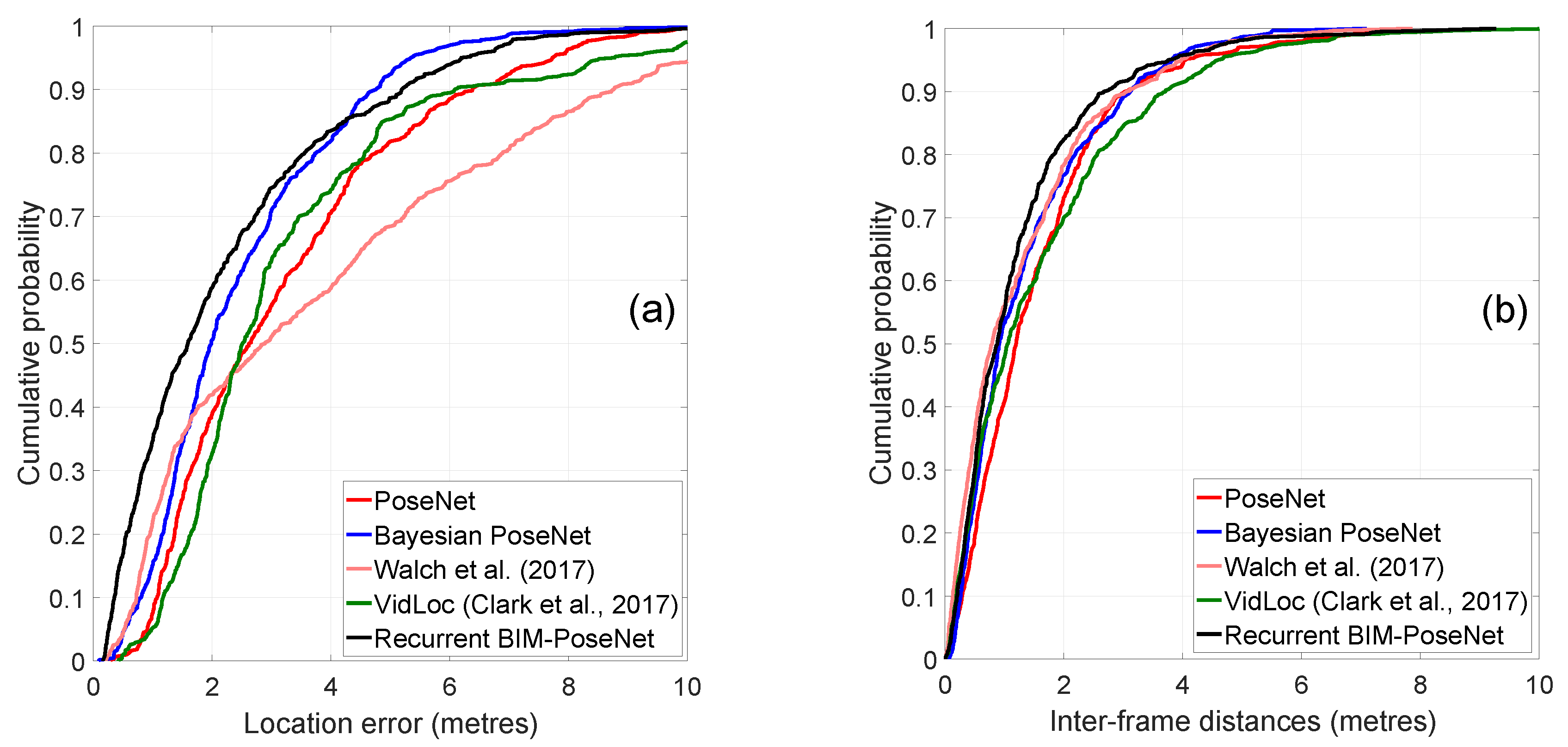
4.4. Experiment 1: Baseline Performance Using Real Image Sequences
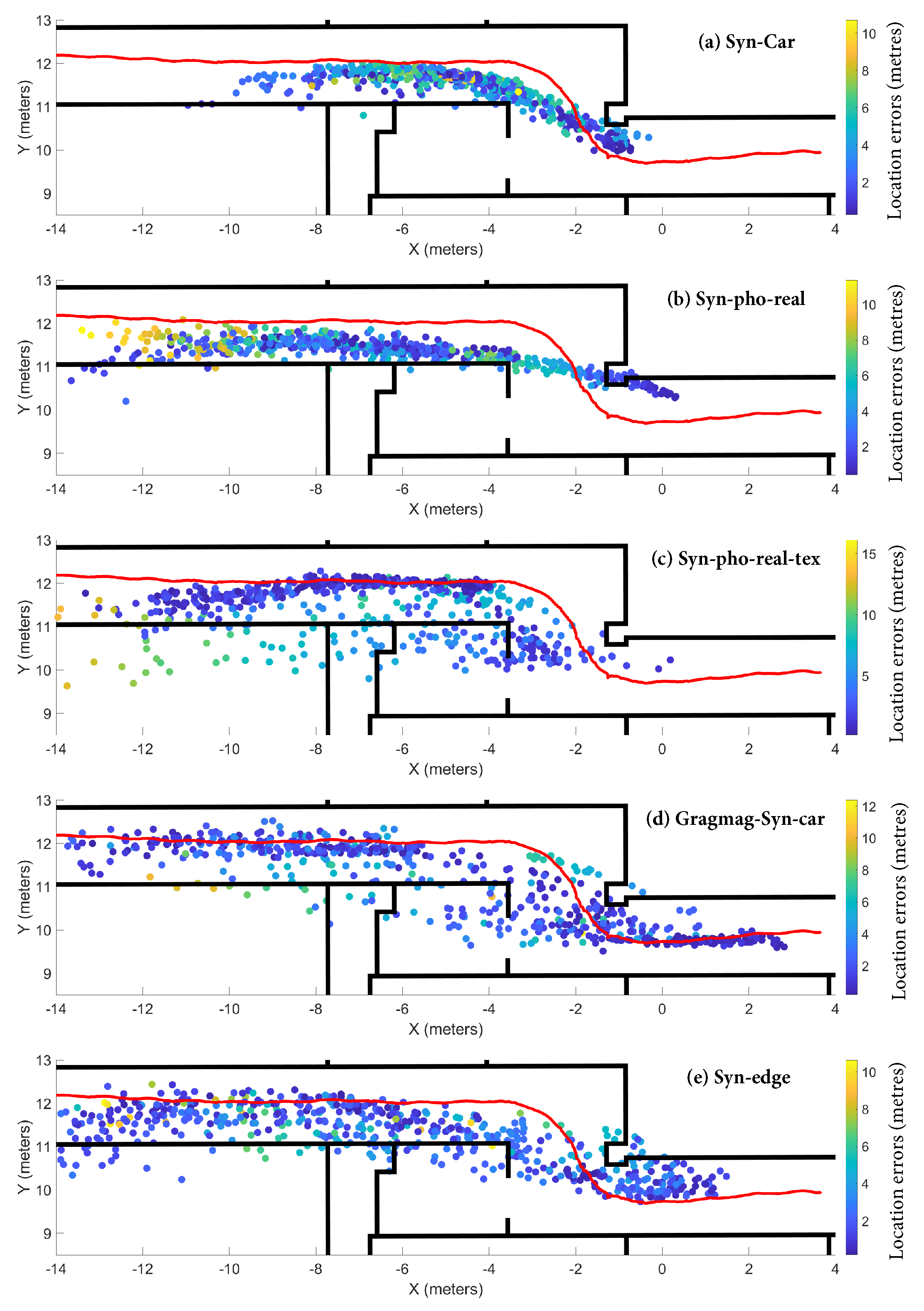
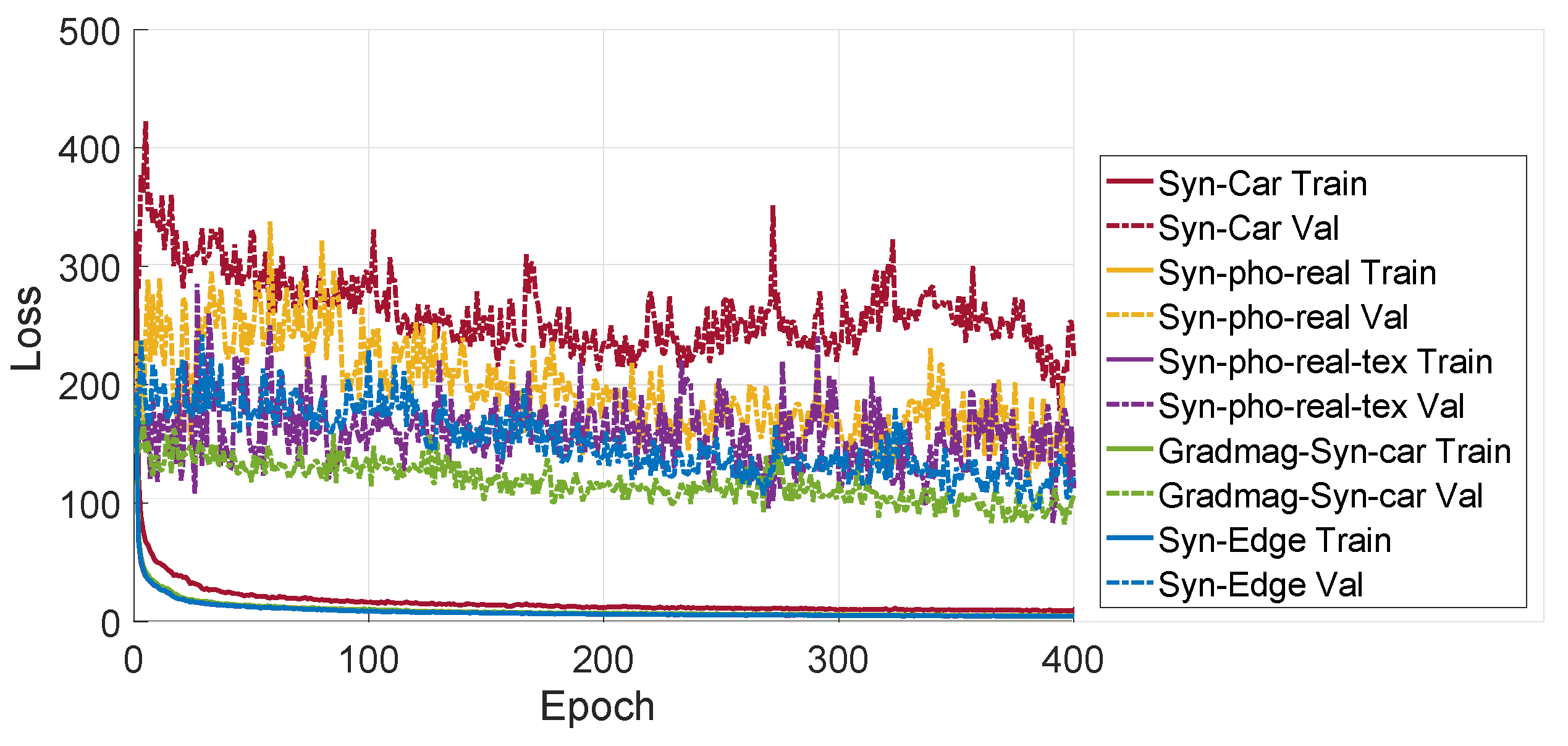
4.5. Experiment 2: Performance of the Network Fine-Tuned Using Synthetic Images and Tested with Real Images
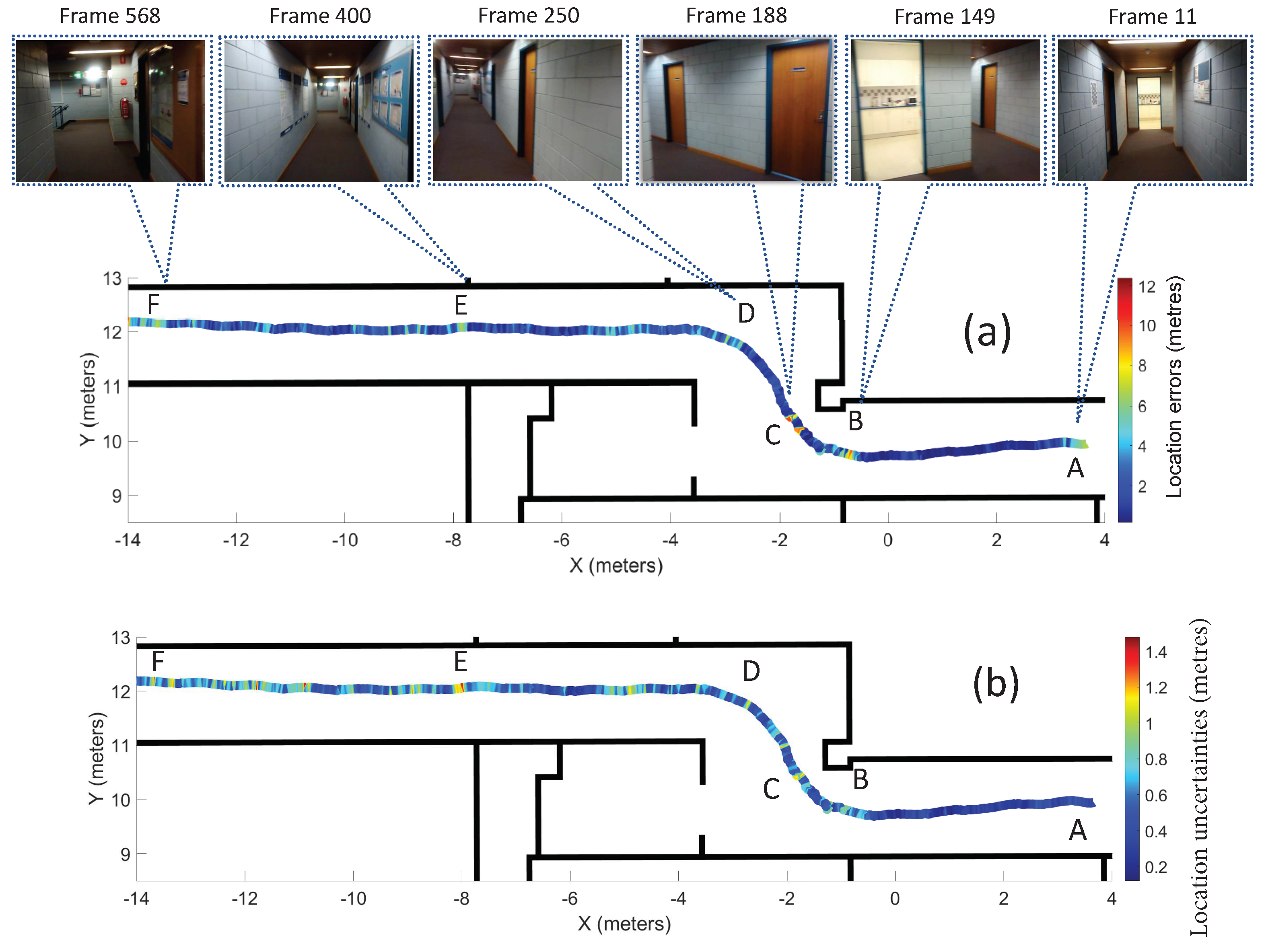
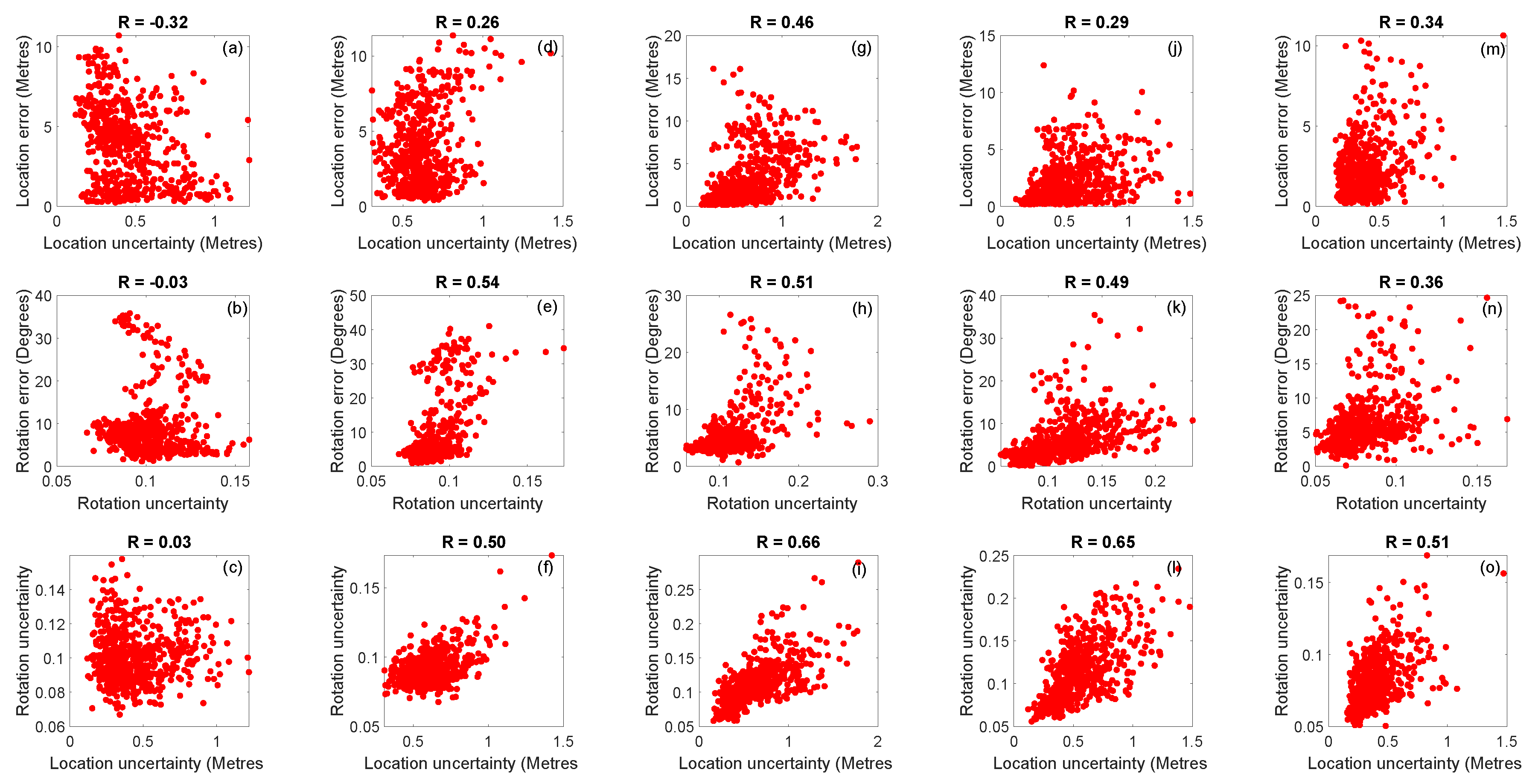
4.6. Experiment 3: Modelling Uncertainty Using Synthetic Images
4.7. Computation Times
5. Conclusions
Supplementary Materials
Author Contributions
Funding
Acknowledgments
Conflicts of Interest
References
- Kendall, A.; Grimes, M.; Cipolla, R. PoseNet: A Convolutional Network for Real-Time 6-DOF Camera Relocalization. In Proceedings of the IEEE International Conference on Computer Vision (ICCV), Santiago, Chile, 7–13 December 2015; pp. 2938–2946. [Google Scholar]
- Kendall, A.; Cipolla, R. Modelling uncertainty in deep learning for camera relocalization. In Proceedings of the IEEE International Conference on Robotics and Automation (ICRA), Stockholm, Sweden, 16–21 May 2016; pp. 4762–4769. [Google Scholar]
- Kendall, A.; Cipolla, R. Geometric loss functions for camera pose regression with deep learning. In Proceedings of the IEEE Conference on Computer Vision and Pattern Recognition (CVPR), Honolulu, HI, USA, 21–26 July 2017; Volume 3, p. 8. [Google Scholar]
- Walch, F.; Hazirbas, C.; Leal-Taixe, L.; Sattler, T.; Hilsenbeck, S.; Cremers, D. Image-based localization using lstms for structured feature correlation. In Proceedings of the IEEE International Conference on Computer Vision (ICCV), Venice, Italy, 22–29 October 2017; pp. 627–637. [Google Scholar]
- Furukawa, Y.; Ponce, J. Accurate, dense, and robust multiview stereopsis. IEEE Trans. Pattern Anal. Mach. Intell. 2010, 32, 1362–1376. [Google Scholar] [CrossRef] [PubMed]
- Gu, F.; Hu, X.; Ramezani, M.; Acharya, D.; Khoshelham, K.; Valaee, S.; Shang, J. Indoor Localization Improved by Spatial Context—A Survey. ACM Comput. Surv. 2019, 52, 1–35. [Google Scholar] [CrossRef]
- Acharya, D.; Khoshelham, K.; Winter, S. BIM-PoseNet: Indoor camera localisation using a 3D indoor model and deep learning from synthetic images. ISPRS J. Photogramm. Remote. Sens. 2019, 150, 245–258. [Google Scholar] [CrossRef]
- Acharya, D.; Singha Roy, S.; Khoshelham, K.; Winter, S. Modelling uncertainty of single image indoor localisation using a 3D model and deep learning. Isprs Ann. Photogramm. Remote. Sens. Spat. Inf. Sci. 2019, IV-2/W5, 247–254. [Google Scholar] [CrossRef]
- Davison, A.J. Real-time simultaneous localisation and mapping with a single camera. In Proceedings of the IEEE International Conference on Computer Vision (ICCV), Nice, France, 14–17 October 2003; Volume 2, pp. 1403–1410. [Google Scholar]
- Nister, D.; Naroditsky, O.; Bergen, J. Visual odometry. In Proceedings of the IEEE Conference on Computer Vision and Pattern Recognition (CVPR), Washington, DC, USA, 27 June–2 July 2004; Volume 1, pp. 652–659. [Google Scholar]
- Acharya, D.; Ramezani, M.; Khoshelham, K.; Winter, S. BIM-Tracker: A model-based visual tracking approach for indoor localisation using a 3D building model. ISPRS J. Photogramm. Remote. Sens. 2019, 150, 157–171. [Google Scholar] [CrossRef]
- Piasco, N.; Sidibé, D.; Demonceaux, C.; Gouet-Brunet, V. A survey on Visual-Based Localization: On the benefit of heterogeneous data. Pattern Recognit. 2018, 74, 90–109. [Google Scholar]
- Irschara, A.; Zach, C.; Frahm, J.M.; Bischof, H. From structure-from-motion point clouds to fast location recognition. In Proceedings of the IEEE Conference on Computer Vision and Pattern Recognition (CVPR), Miami, FL, USA, 20–25 May 2009; pp. 2599–2606. [Google Scholar]
- Kneip, L.; Scaramuzza, D.; Siegwart, R. A novel parametrization of the perspective-three-point problem for a direct computation of absolute camera position and orientation. In Proceedings of the IEEE Conference on Computer Vision and Pattern Recognition (CVPR), Colorado Springs, CO, USA, 20–25 June 2011; pp. 2969–2976. [Google Scholar]
- Shotton, J.; Glocker, B.; Zach, C.; Izadi, S.; Criminisi, A.; Fitzgibbon, A. Scene Coordinate Regression Forests for Camera Relocalization in RGB-D Images. In Proceedings of the IEEE Conference on Computer Vision and Pattern Recognition (CVPR), Portland, OR, USA, 23–28 June 2013; pp. 2930–2937. [Google Scholar]
- Brachmann, E.; Rother, C. Learning less is more-6d camera localization via 3d surface regression. In Proceedings of the IEEE Conference on Computer Vision and Pattern Recognition, Salt Lake City, UT, USA, 18–22 June 2018; pp. 4654–4662. [Google Scholar]
- Cavallari, T.; Golodetz, S.; Lord, N.A.; Valentin, J.; Di Stefano, L.; Torr, P.H. On-the-fly adaptation of regression forests for online camera relocalisation. In Proceedings of the IEEE conference on computer vision and pattern recognition, Honolulu, HI, USA, 21–26 July 2017; pp. 4457–4466. [Google Scholar]
- Brachmann, E.; Krull, A.; Nowozin, S.; Shotton, J.; Michel, F.; Gumhold, S.; Rother, C. Dsac-differentiable ransac for camera localization. In Proceedings of the IEEE Conference on Computer Vision and Pattern Recognition, Honolulu, HI, USA, 21–26 July 2017; pp. 6684–6692. [Google Scholar]
- Wu, J.; Ma, L.; Hu, X. Delving deeper into convolutional neural networks for camera relocalization. In Proceedings of the IEEE International Conference on Robotics and Automation (ICRA), Singapore, 29 May–3 June 2017; pp. 5644–5651. [Google Scholar]
- Clark, R.; Wang, S.; Markham, A.; Trigoni, N.; Wen, H. VidLoc: A deep spatio-temporal model for 6-dof video-clip relocalization. In Proceedings of the IEEE Conference on Computer Vision and Pattern Recognition (CVPR), Honolulu, HI, USA, 21–26 July 2017; Volume 3. [Google Scholar]
- Ha, I.; Kim, H.; Park, S.; Kim, H. Image retrieval using BIM and features from pretrained VGG network for indoor localization. Build. Environ. 2018, 140, 23–31. [Google Scholar] [CrossRef]
- Szegedy, C.; Liu, W.; Jia, Y.; Sermanet, P.; Reed, S.; Anguelov, D.; Erhan, D.; Vanhoucke, V.; Rabinovich, A. Going Deeper With Convolutions. In Proceedings of the IEEE Conference on Computer Vision and Pattern Recognition (CVPR), Boston, MA, USA, 7–12 June 2015; pp. 1–9. [Google Scholar]
- Hochreiter, S.; Schmidhuber, J. Long short-term memory. Neural Comput. 1997, 9, 1735–1780. [Google Scholar] [CrossRef] [PubMed]
- Szegedy, C.; Vanhoucke, V.; Ioffe, S.; Shlens, J.; Wojna, Z. Rethinking the inception architecture for computer vision. In Proceedings of the IEEE conference on computer vision and pattern recognition, Las Vegas, NV, USA, 27–30 June 2016; pp. 2818–2826. [Google Scholar]
- Zhou, B.; Lapedriza, A.; Xiao, J.; Torralba, A.; Oliva, A. Learning deep features for scene recognition using places database. In Proceedings of the Advances in Neural Information Processing Systems, Montreal, QC, Canada, 8–13 December 2014; pp. 487–495. [Google Scholar]
- Zhu, L.; Laptev, N. Deep and confident prediction for time series at uber. In Proceedings of the 2017 IEEE International Conference on Data Mining Workshops (ICDMW), New Orleans, LA, USA, 28–21 November 2017; pp. 103–110. [Google Scholar]
- Gal, Y.; Ghahramani, Z. Bayesian convolutional neural networks with Bernoulli approximate variational inference. arXiv 2015, arXiv:1506.02158. [Google Scholar]
- Chollet, F. Keras. 2015. Available online: https://keras.io (accessed on 15 August 2020).
- Abadi, M.; Agarwal, A.; Barham, P.; Brevdo, E.; Chen, Z. TensorFlow: Large-Scale Machine Learning on Heterogeneous Systems. 2015. Available online: tensorflow.org (accessed on 15 August 2020).
- Khoshelham, K.; Vilariño, L.D.; Peter, M.; Kang, Z.; Acharya, D. The isprs benchmark on indoor modelling. Int. Arch. Photogramm. Remote. Sens. Spat. Inf. Sci. 2017, 42, 367–372. [Google Scholar] [CrossRef]
- Ramezani, M.; Acharya, D.; Gu, F.; Khoshelham, K. Indoor positioning by visual-inertial odometry. ISPRS Ann. Photogramm. Remote. Sens. Spat. Inf. Sci. 2017, 4, 371–376. [Google Scholar]
- Khoshelham, K.; Tran, H.; Vilariño, L.D.; Peter, M.; Kang, Z.; Acharya, D. An evaluation framework for benchmarking indoor modelling methods. ISPRS Int. Arch. Photogramm. Remote. Sens. Spat. Inf. Sci. 2018, XLII-4, 297–302. [Google Scholar] [CrossRef]
- Tran, H.; Khoshelham, K.; Kealy, A. Geometric comparison and quality evaluation of 3D models of indoor environments. ISPRS J. Photogramm. Remote. Sens. 2019, 149, 29–39. [Google Scholar] [CrossRef]
- Volk, R.; Stengel, J.; Schultmann, F. Building Information Modeling (BIM) for existing buildings—Literature review and future needs. Autom. Constr. 2014, 38, 109–127. [Google Scholar] [CrossRef]
- Porwal, A.; Hewage, K.N. Building Information Modeling (BIM) partnering framework for public construction projects. Autom. Constr. 2013, 31, 204–214. [Google Scholar] [CrossRef]
- Gal, Y.; Ghahramani, Z. A theoretically grounded application of dropout in recurrent neural networks. In Proceedings of the Advances in Neural Information Processing Systems, Barcelona, Spain, 5–10 December 2016; pp. 1019–1027. [Google Scholar]
- Sehgal, A.; Kehtarnavaz, N. Guidelines and Benchmarks for Deployment of Deep Learning Models on Smartphones as Real-Time Apps. Mach. Learn. Knowl. Extr. 2019, 1, 450–465. [Google Scholar] [CrossRef]
- Long, J.; Shelhamer, E.; Darrell, T. Fully convolutional networks for semantic segmentation. In Proceedings of the IEEE Conference on Computer Vision and Pattern Recognition, Boston, MA, USA, 7–12 June 2015; pp. 3431–3440. [Google Scholar]


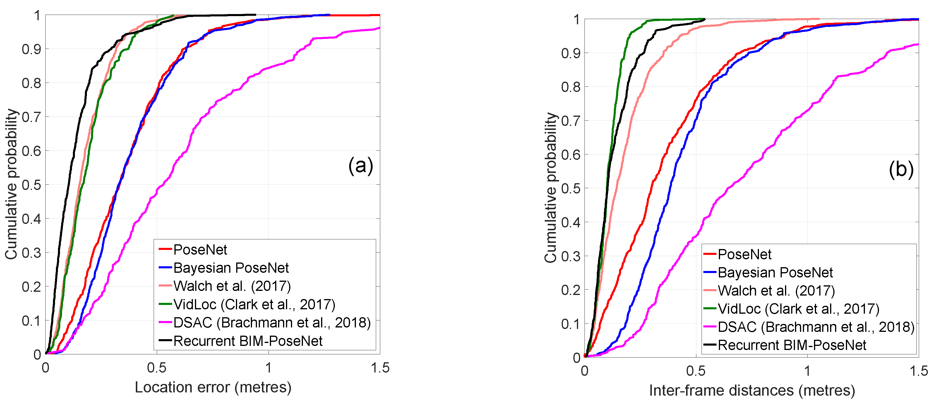
| Approach | Errors (Metres, Degrees) | Inter-Frame Distances (Metres) |
|---|---|---|
| PoseNet [1] | m, 1.85 | m |
| Bayesian PoseNet [2] | m, 1.53 | m |
| DSAC++ [16] | m, 0.61 | m |
| Walch et al. [4] | m, 1.62 | m |
| VidLoc [20] | m, 0.87 | m |
| Recurrent BIM-PoseNet (ours) | m, 0.83 | m |
| Approach | Syn-Car | Syn-Pho-Real | Syn-Pho-Real-Tex | Gradmag-Syn-Car | Syn-Edge |
|---|---|---|---|---|---|
| BIM-PoseNet | m, 37.16 | m, 11.33 | m, 12.25 | m, 6.99 | m, 7.73 |
| Bayesian BIM-PoseNet | m, 8.38 | m, 25.03 | m, 13.53 | m, 7.33 | m, 12.53 |
| Walch et al. [4] | m, 22.28 | m, 15.31 | m, 11.99 | m, 19.22 | m, 12.42 |
| VidLoc [20] | m, 11.81 | m, 11.45 | m, 11.12 | m, 11.42 | m, 7.26 |
| Recurrent BIM-PoseNet | m, 15.20 | m, 8.50 | m, 8.31 | m, 9.29 | m, 11.15 |
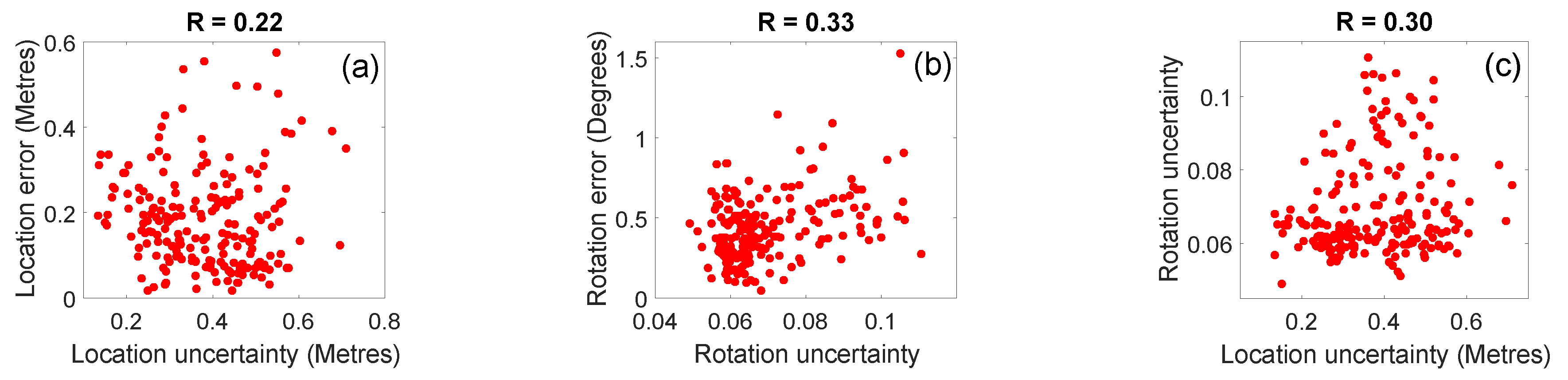
| Frame | Location Error (Metre) | Location Uncertainties (Metre) | Rotation Error | Rotational Uncertainty |
|---|---|---|---|---|
| 11 | 6.82 | 0.36 | 4.52 | 0.09 |
| 149 | 7.60 | 0.41 | 2.85 | 0.08 |
| 188 | 9.11 | 0.73 | 30.61 | 0.16 |
| 250 | 5.92 | 0.68 | 9.67 | 0.14 |
| 400 | 6.45 | 0.53 | 4.51 | 0.09 |
| 568 | 6.91 | 0.53 | 15.16 | 0.12 |
| Fine-Tuned on | Bayesian | Recurrent | ||||
|---|---|---|---|---|---|---|
| BIM-PoseNet | BIM-PoseNet | |||||
| Syn-car | 0.12 | 0.31 | 0.34 | −0.32 | −0.03 | 0.03 |
| Syn-pho-real | 0.36 | −0.01 | 0.04 | 0.26 | 0.54 | 0.50 |
| Syn-pho-real-tex | 0.33 | 0.53 | 0.33 | 0.46 | 0.51 | 0.66 |
| Gradmag-Syn-car | 0.42 | 0.50 | 0.59 | 0.29 | 0.49 | 0.65 |
| Syn-edge | 0.46 | 0.40 | 0.41 | 0.34 | 0.36 | 0.51 |
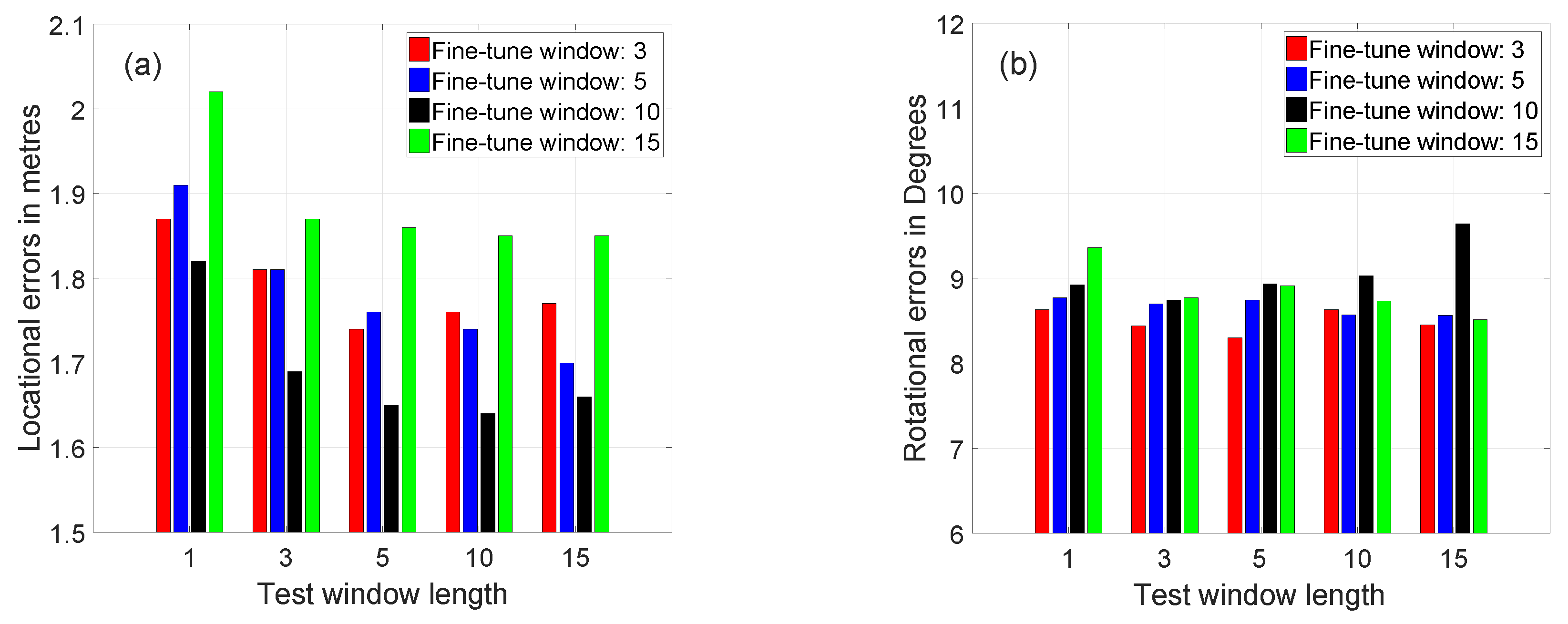
| Window Length | Fine-Tune Time (Hrs) | Test Time GPU (ms) | Test Time CPU (s) |
|---|---|---|---|
| 1 | 1:44 | 12 | 0.13 |
| 3 | 4:34 | 16 | 0.40 |
| 5 | 7:07 | 35 | 0.67 |
| 10 | 12:43 | 52 | 0.94 |
| 15 | 23:48 | 108 | 2.12 |
© 2020 by the authors. Licensee MDPI, Basel, Switzerland. This article is an open access article distributed under the terms and conditions of the Creative Commons Attribution (CC BY) license (http://creativecommons.org/licenses/by/4.0/).
Share and Cite
Acharya, D.; Singha Roy, S.; Khoshelham, K.; Winter, S. A Recurrent Deep Network for Estimating the Pose of Real Indoor Images from Synthetic Image Sequences. Sensors 2020, 20, 5492. https://doi.org/10.3390/s20195492
Acharya D, Singha Roy S, Khoshelham K, Winter S. A Recurrent Deep Network for Estimating the Pose of Real Indoor Images from Synthetic Image Sequences. Sensors. 2020; 20(19):5492. https://doi.org/10.3390/s20195492
Chicago/Turabian StyleAcharya, Debaditya, Sesa Singha Roy, Kourosh Khoshelham, and Stephan Winter. 2020. "A Recurrent Deep Network for Estimating the Pose of Real Indoor Images from Synthetic Image Sequences" Sensors 20, no. 19: 5492. https://doi.org/10.3390/s20195492
APA StyleAcharya, D., Singha Roy, S., Khoshelham, K., & Winter, S. (2020). A Recurrent Deep Network for Estimating the Pose of Real Indoor Images from Synthetic Image Sequences. Sensors, 20(19), 5492. https://doi.org/10.3390/s20195492