Facial Muscle Activity Recognition with Reconfigurable Differential Stethoscope-Microphones
Abstract
1. Introduction
1.1. Paper Contribution
- We put forward the idea of using differential sound analysis as an unobtrusive way of acquiring information about facial muscle activity patterns and the associated facial expressions and actions.
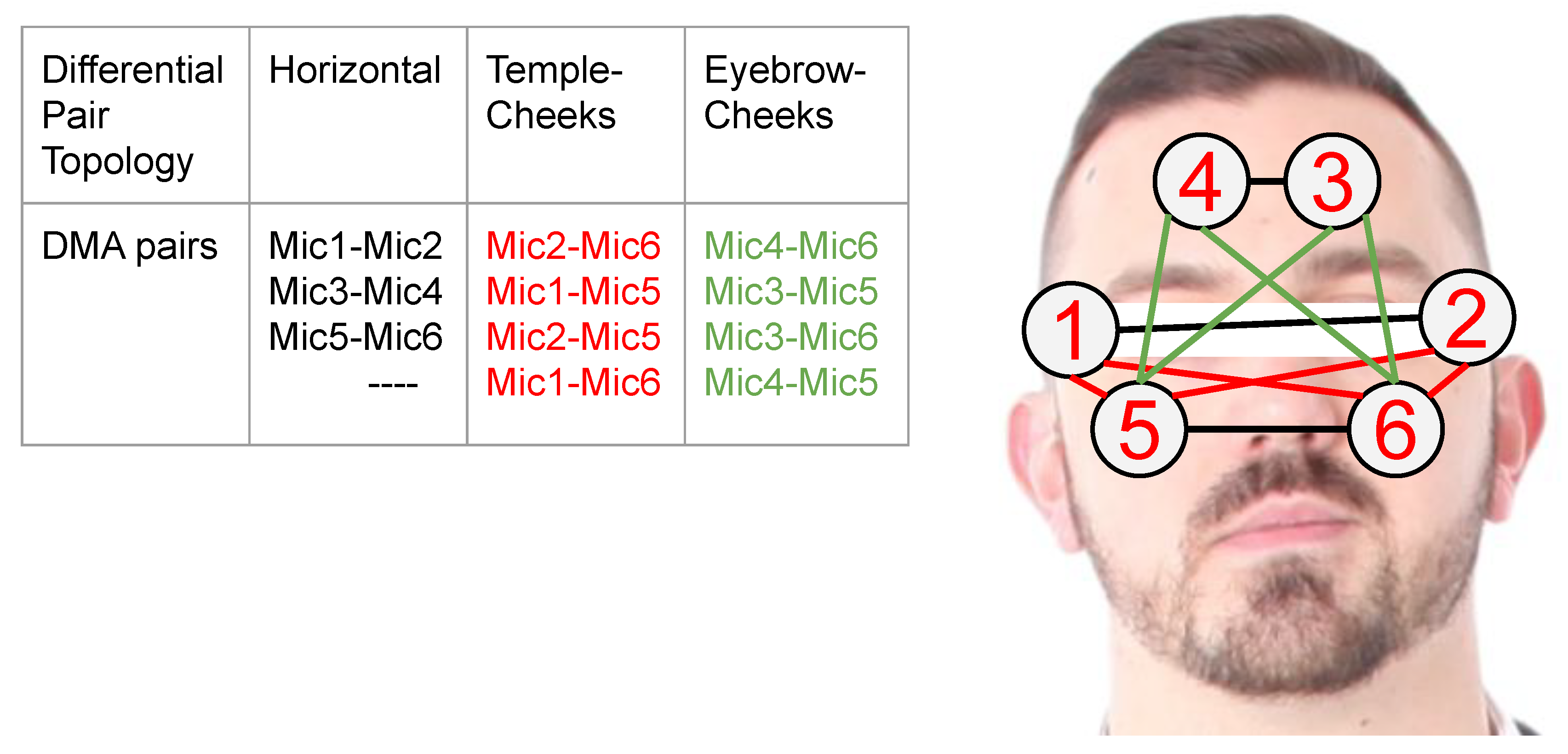
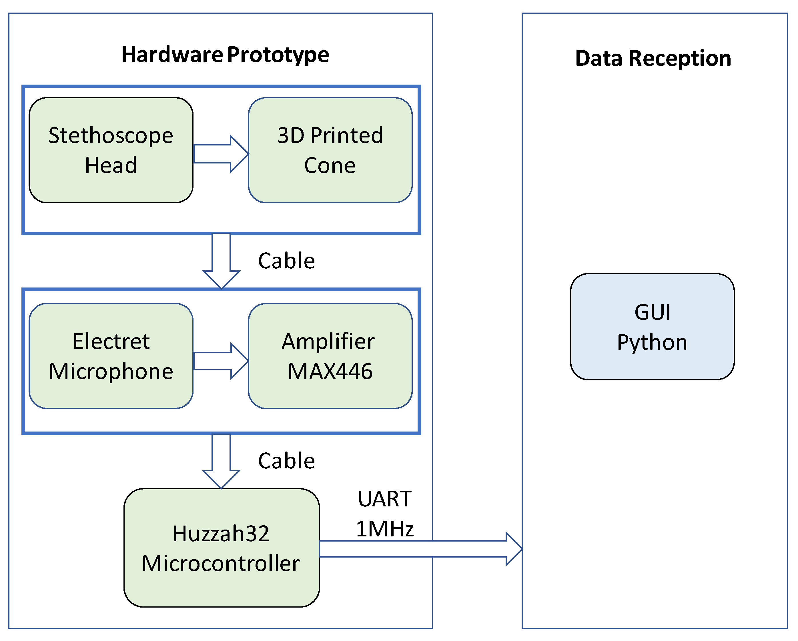
- We present the design and implementation of a reconfigurable signal acquisition system based on that idea. It consists of six stethoscopes at positions that are compatible with a smart glasses frame (see Figure 1).
- We present an in-depth analysis of the system’s characteristics and the signals for various facial actions.
- We describe the design and implementation of the entire processing pipeline needed to go from signal pre-processing to recognizing complex facial actions, including a study of the significance of different features, derived from combinations of six stethoscopes (at a set of locations that are inspired by a typical glasses frame). Additionally, the selection of best-suited ML methods.
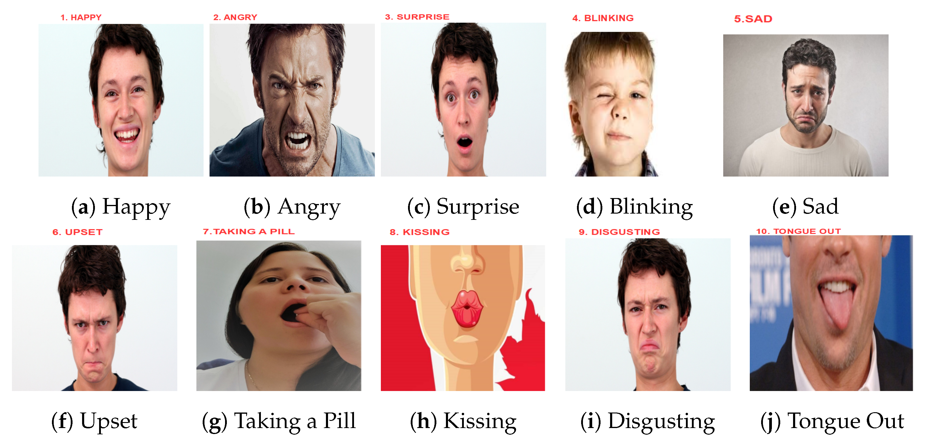
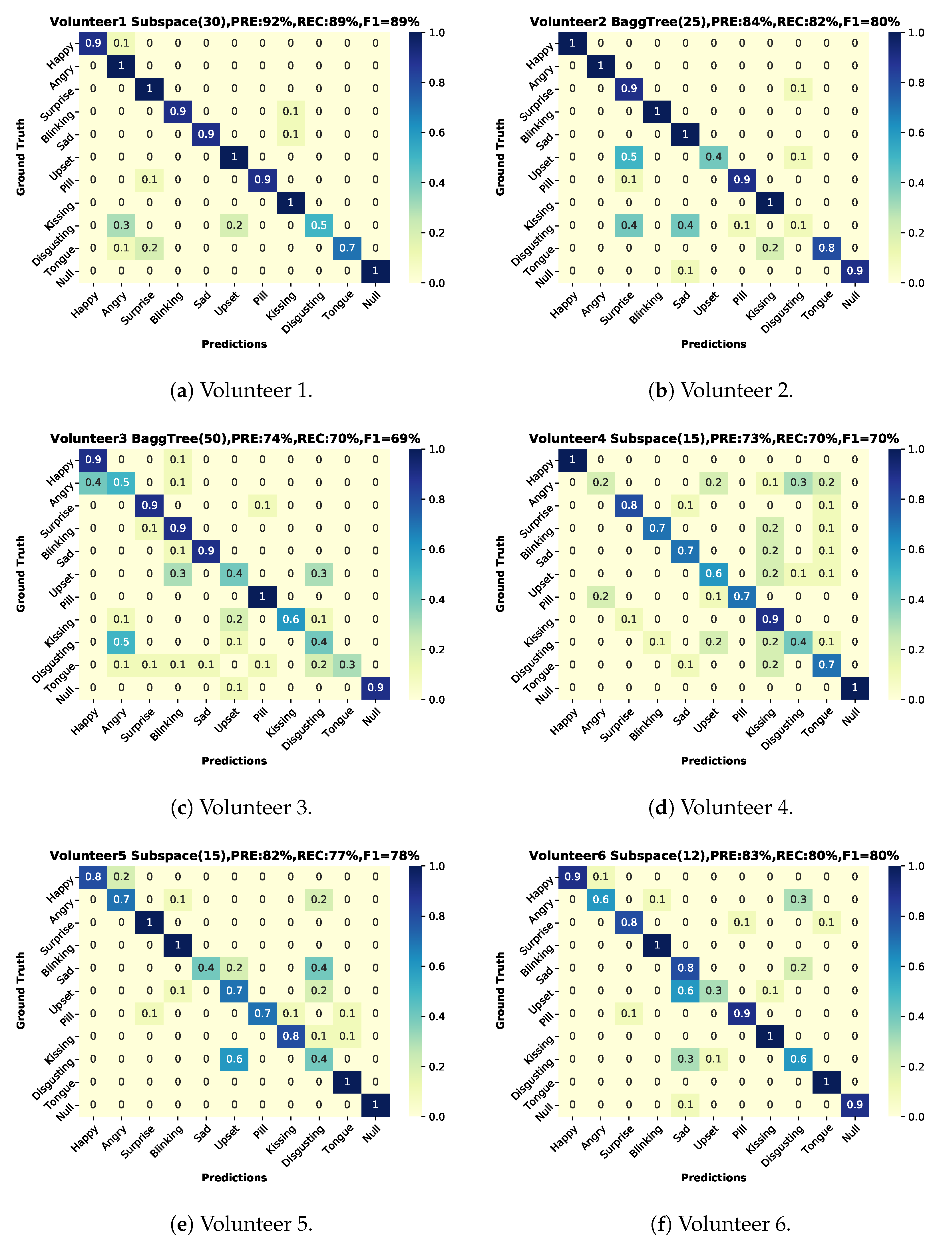
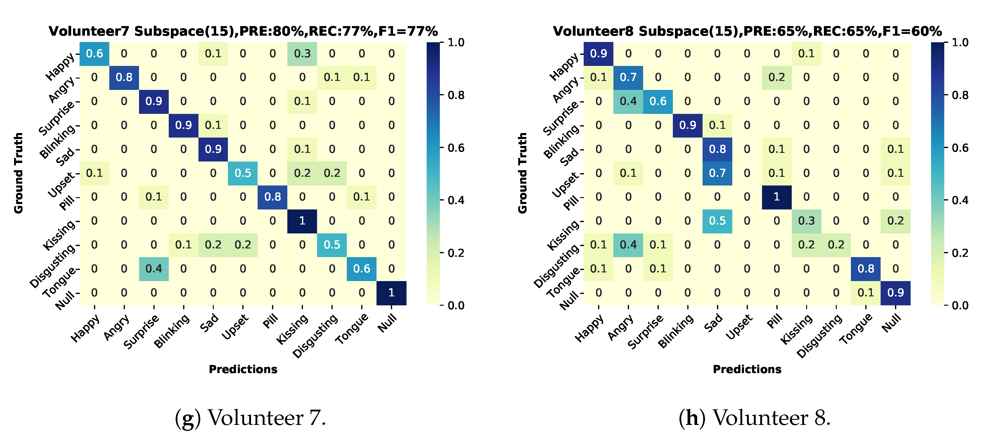
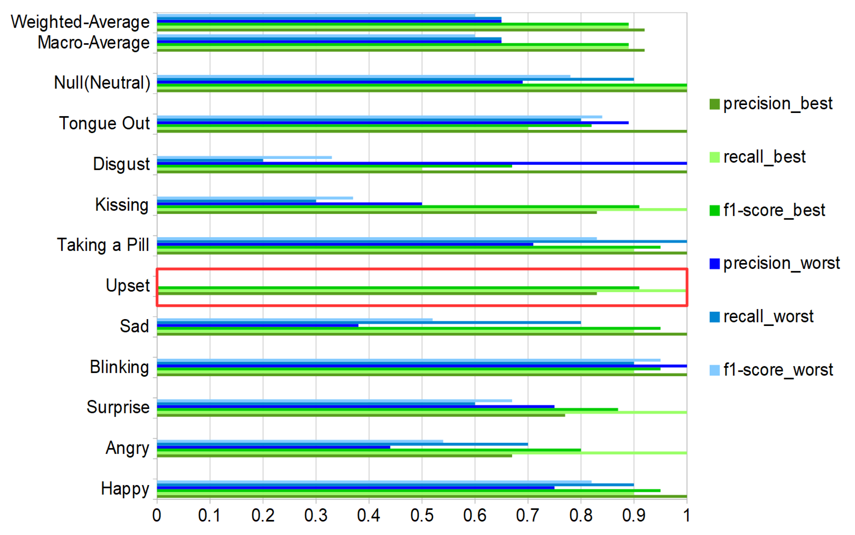
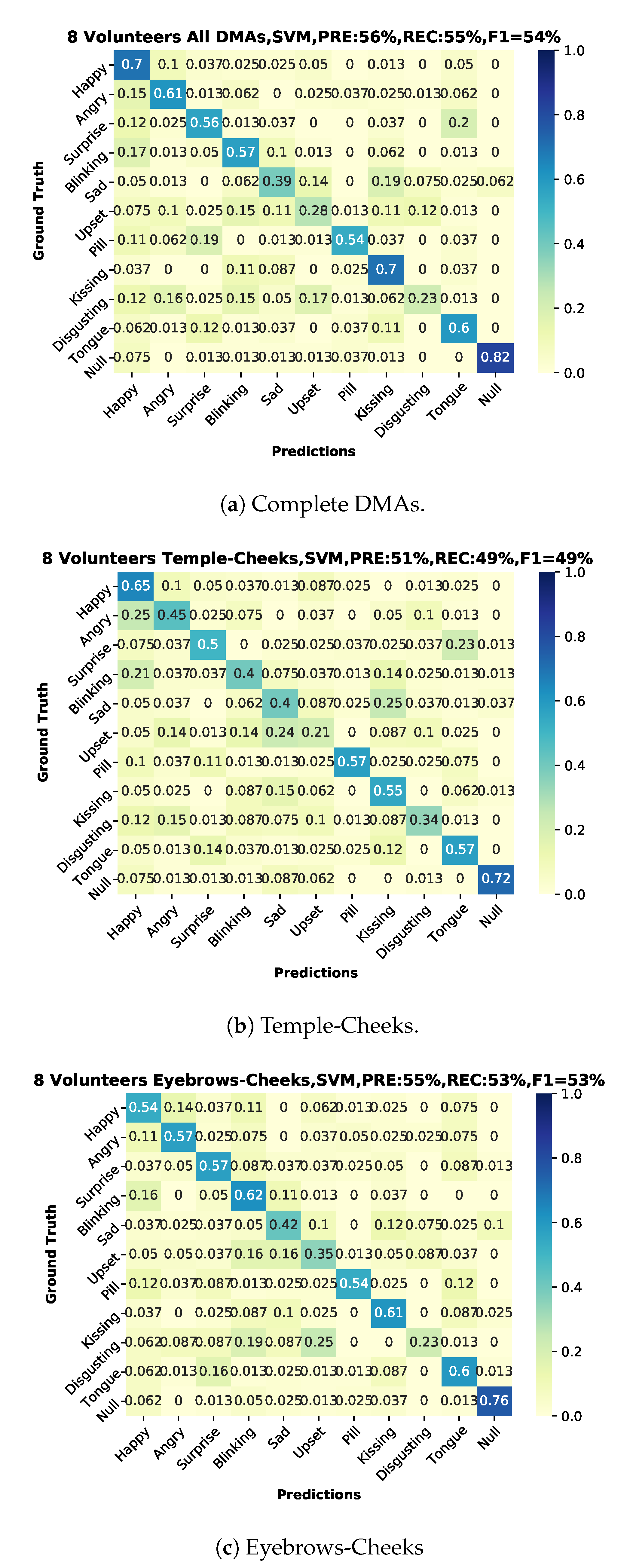
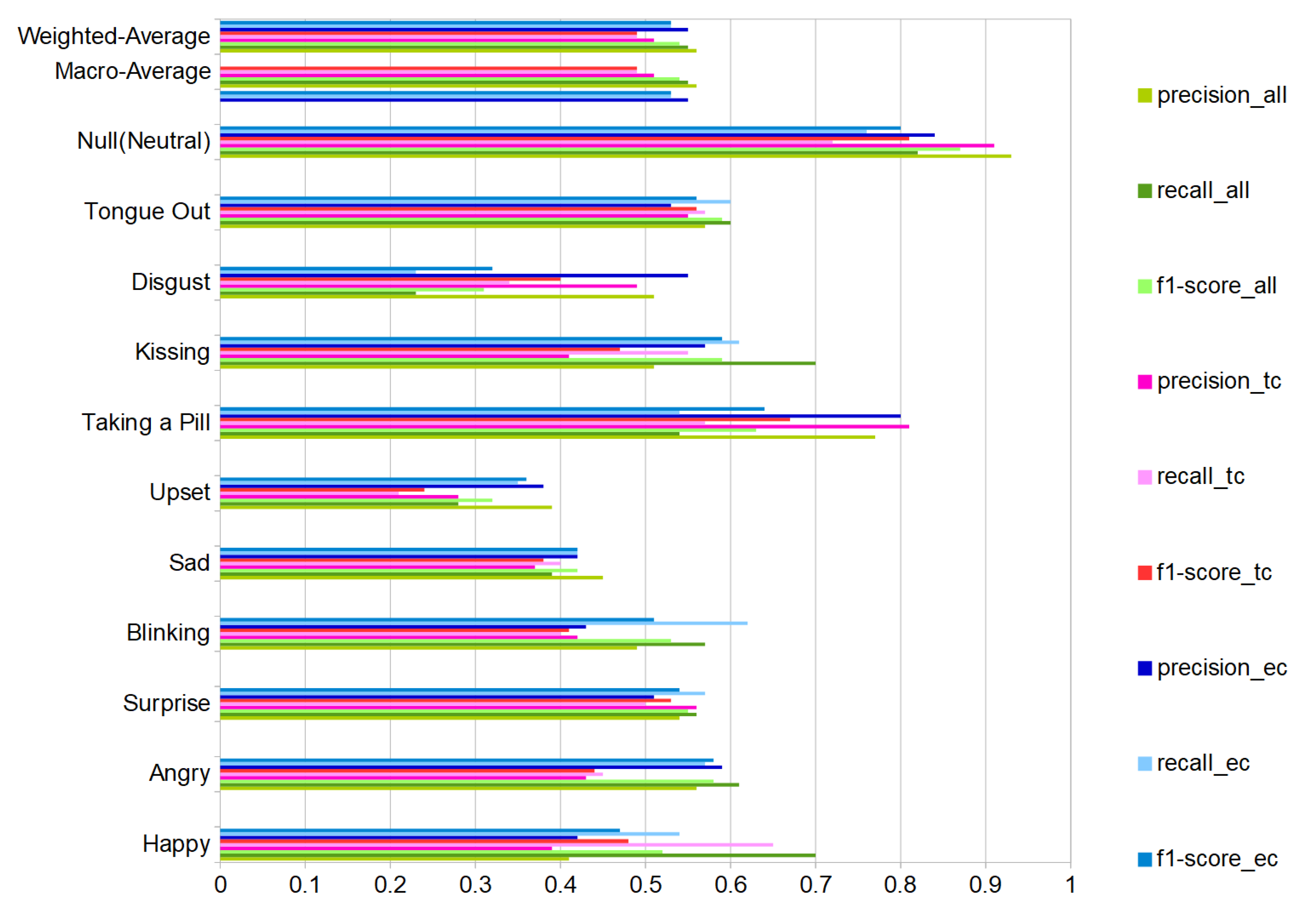
- We have conducted a systematic evaluation with eight users mimicking a set of 10 common facial expressions and actions (plus a NULL class of neutral face), as shown in Figure 2. Each user has recorded three sessions of 10 repetitions of each action for a total of 2640 events. Using a leave-session-out evaluation scheme across all users, we achieve an f1-score equal to 54% (9% chance-level) for those ten classes plus the non-interest class defined as “Neutral-face”. In the user-dependent case, we achieved an f1-score between 60% and 89% (9% chance-level), reflecting that not all users were equally good at mimicking specific actions.
1.2. Paper Structure
2. Background and Related Work
2.1. Wearable Facial Sensing
2.2. Microphone-Stethoscope
2.3. Differential Microphone Arrays (DMAs)
2.4. Acoustic Mechanomyography (A-MMG)
2.5. Facial Expressions
3. Audio Design and Hardware
3.1. Differential Microphone Array Configuration
3.2. Calibration Procedure
3.2.1. Single Microphones Discrete Frequency Response Calibration
- DMA 1st order with matching factor is called :
- By substitution of in :
- Assuming same sound source position and geometry, only gain discrepancies.
- By substitution of in .
3.2.2. Differential Microphones Discrete Frequency Response Calibration
3.3. System Architecture and Implementation
4. Detecting Expression Experiment Design
4.1. Facial Expressions
4.2. Participants
4.3. Experiment Procedure
5. Data Analysis
5.1. Feature Extraction
- F1 quantile
- F2 quantile
- F3 Absolute FFT coefficient
- F4 Absolute FFT coefficient
- F5 Absolute FFT coefficient
- F6 p-Value of Linear Trend
- F7 Standard-Error of Linear Trend
- F8 Energy ratio by chunks (num-segments = 10, segment-focus = 1)
- F9 Energy ratio by chunks (num-segments = 10, segment-focus = 8)
- F10 Autocorrelation of lag = 2
- F11 c3 = lag = 3
- F12 Count below mean
- F13 Minimum R-Value of Linear Trend (chunk-length = 10)
- F14 Largest fixed point of dynamics (PolyOrder = 3, #quantile = 30)
- F15 Ratio beyond r-sigma (r = 1.5)
- F16 Mean change quantiles with absolute difference (qH = 1.0, qL = 0.0)
5.2. Classifier Selection
6. Evaluation Results
6.1. User-Dependent Test
6.2. User-Independent Test
6.3. Discussion
6.3.1. Overall Results
6.3.2. User Dependence
- Physiological differences between users.
- Different ways users may express specific actions.
- Related to the above point, the inability of some subjects to mimic specific actions accurately.
6.3.3. Gesture/Action Dependence
6.3.4. Comparison with Other Published Approaches
7. Conclusions and Future Work
- Using differential signals between suitable pairs of microphones is a key feature of our system. This is probably related to the fact that it captures temporal patterns of muscle activation rather than a precise sound corresponding to the specific type of activation of a particular muscle. It also helps us deal with inter person variability and noise.
- The eyebrows-cheeks’ positions are the most informative locations for most of the investigated gestures and actions.
- Using a stethoscope like sound acquisition setup has significantly improved the signal quality.
- In our tests, we used a “train on all-test on all” approach, which demonstrates that the method has a degree of user independence. On the other hand, we have also seen a strong dependency on the person’s ability to recognize and mimic the expressions with the best user reaching an f1-score = 89% and the worst one being 60%.
Author Contributions
Funding
Conflicts of Interest
References
- Ko, B. A Brief Review of Facial Emotion Recognition Based on Visual Information. Sensors 2018, 18, 401. [Google Scholar] [CrossRef] [PubMed]
- Aspandi, D.; Martinez, O.; Sukno, F.; Binefa, X. Fully End-to-End Composite Recurrent Convolution Network for Deformable Facial Tracking InThe Wild. In Proceedings of the 2019 14th IEEE International Conference on Automatic Face Gesture Recognition (FG 2019), Lille, France, 14–18 May 2019; pp. 1–8. [Google Scholar]
- Bao, Q.; Luan, F.; Yang, J. Improving the accuracy of beamforming method for moving acoustic source localization in far-field. In Proceedings of the 2017 10th International Congress on Image and Signal Processing, BioMedical Engineering and Informatics (CISP-BMEI), Shanghai, China, 14–16 October 2017; pp. 1–6. [Google Scholar] [CrossRef]
- Chen, T.; Huang, Q.; Zhang, L.; Fang, Y. Direction of Arrival Estimation Using Distributed Circular Microphone Arrays. In Proceedings of the 2018 14th IEEE International Conference on Signal Processing (ICSP), Beijing, China, 12–16 August 2018; pp. 182–185. [Google Scholar] [CrossRef]
- Marur, T.; Tuna, Y.; Demirci, S. Facial anatomy. Clin. Dermatol. 2014, 32, 14–23. [Google Scholar] [CrossRef] [PubMed]
- Olszanowski, M.; Pochwatko, G.; Kuklinski, K.; Scibor-Rylski, M.; Lewinski, P.; Ohme, R. Warsaw Set of Emotional Facial Expression Pictures: A validation study of facial display photographs. Front. Psychol. 2014, 5. [Google Scholar] [CrossRef] [PubMed]
- Hugh Jackman|Wolverine Hugh Jackman, Hugh Jackman, Jackman. Available online: https://www.pinterest.de/pin/361765782554181392/ (accessed on 22 June 2020).
- Doc2Us - Your Personal Pocket Doctor. Available online: https://www.doc2us.com/8-whys-your-toddler-blinking-hard-complete-list (accessed on 22 June 2020).
- 25 Celebrities Sticking Out Their Tongues|Brad Pitt, Stick It Out, George Clooney. Available online: https://www.pinterest.de/pin/243757398561743241/ (accessed on 22 June 2020).
- Canadian Kiss Stock-Illustration—Getty Images. Available online: https://www.gettyimages.de/detail/illustration/canadian-kiss-lizenfreie-illustration/472283539?adppopup=true (accessed on 6 July 2020).
- Scheirer, J.; Fern, R.; Picard, R. Expression Glasses: A Wearable Device for Facial Expression Recognition. In Proceedings of the CHI’99 Extended Abstracts on Human Factors in Computing Systems, Pittsburgh, PA, USA, 15–20 May 1999. [Google Scholar] [CrossRef]
- Masai, K.; Sugiura, Y.; Ogata, M.; Kunze, K.; Inami, M.; Sugimoto, M. Facial Expression Recognition in Daily Life by Embedded Photo Reflective Sensors on Smart Eyewear. In Proceedings of the 21st International Conference on Intelligent User Interfaces, Sonoma, CA, USA, 7–10 March 2016; pp. 317–326. [Google Scholar] [CrossRef]
- Fu, Y.; Luo, J.; Nguyen, N.; Walton, A.; Flewitt, A.; Zu, X.; Li, Y.; McHale, G.; Matthews, A.; Iborra, E.; et al. Advances in piezoelectric thin films for acoustic biosensors, acoustofluidics and lab-on-chip applications. Prog. Mater. Sci. 2017, 89, 31–91. [Google Scholar] [CrossRef]
- Gruebler, A.; Suzuki, K. Design of a Wearable Device for Reading Positive Expressions from Facial EMG Signals. IEEE Trans. Affect. Comput. 2014, 5, 227–237. [Google Scholar] [CrossRef]
- Perusquía-Hernández, M.; Hirokawa, M.; Suzuki, K. A Wearable Device for Fast and Subtle Spontaneous Smile Recognition. IEEE Trans. Affect. Comput. 2017, 8, 522–533. [Google Scholar] [CrossRef]
- Lamkin-Kennard, K.A.; Popovic, M.B. 4—Sensors: Natural and Synthetic Sensors. In Biomechatronics; Popovic, M.B., Ed.; Academic Press: Cambridge, MA, USA, 2019; pp. 81–107. [Google Scholar] [CrossRef]
- Zhou, B.; Ghose, T.; Lukowicz, P. Expressure: Detect Expressions Related to Emotional and Cognitive Activities Using Forehead Textile Pressure Mechanomyography. Sensors 2020, 20, 730. [Google Scholar] [CrossRef]
- Pavlosky, A.; Glauche, J.; Chambers, S.; Al-Alawi, M.; Yanev, K.; Loubani, T. Validation of an effective, low cost, Free/open access 3D-printed stethoscope. PLoS ONE 2018, 13, e0193087. [Google Scholar] [CrossRef]
- Huang, H.; Yang, D.; Yang, X.; Lei, Y.; Chen, Y. Portable multifunctional electronic stethoscope. In Proceedings of the 2019 IEEE 3rd Information Technology, Networking, Electronic and Automation Control Conference (ITNEC), Chengdu, China, 15–17 March 2019; pp. 691–694. [Google Scholar] [CrossRef]
- Aguilera-Astudillo, C.; Chavez-Campos, M.; Gonzalez-Suarez, A.; Garcia-Cordero, J.L. A low-cost 3-D printed stethoscope connected to a smartphone. In Proceedings of the 2016 38th Annual International Conference of the IEEE Engineering in Medicine and Biology Society (EMBC), Orlando, FL, USA, 16–20 August 2016; pp. 4365–4368. [Google Scholar] [CrossRef]
- Sumarna, S.; Astono, J.; Purwanto, A.; Agustika, D.K. The improvement of phonocardiograph signal (PCG) representation through the electronic stethoscope. In Proceedings of the 2017 4th International Conference on Electrical Engineering, Computer Science and Informatics (EECSI), Yogyakarta, Indonesia, 19–21 September 2017; pp. 1–5. [Google Scholar] [CrossRef]
- Ou, D.; OuYang, L.; Tan, Z.; Mo, H.; Tian, X.; Xu, X. An electronic stethoscope for heart diseases based on micro-electro-mechanical-system microphone. In Proceedings of the 2016 IEEE 14th International Conference on Industrial Informatics (INDIN), Poitiers, France, 19–21 July 2016; pp. 882–885. [Google Scholar] [CrossRef]
- Malik, B.; Eya, N.; Migdadi, H.; Ngala, M.J.; Abd-Alhameed, R.A.; Noras, J.M. Design and development of an electronic stethoscope. In Proceedings of the 2017 Internet Technologies and Applications (ITA), Wrexham, UK, 12–15 September 2017; pp. 324–328. [Google Scholar] [CrossRef]
- Kusainov, R.K.; Makukha, V.K. Evaluation of the applicability of MEMS microphone for auscultation. In Proceedings of the 2015 16th International Conference of Young Specialists on Micro/Nanotechnologies and Electron Devices, Erlagol, Russia, 29 June–3 July 2015; pp. 595–597. [Google Scholar] [CrossRef]
- Paul Yang, J.C. Electronic Stethoscope with Piezo-Electrical Film Contact Microphone. U.S. Patent No. 2005/0157888A1, 16 January 2004. [Google Scholar]
- Charlier, P.; Herman, C.; Rochedreux, N.; Logier, R.; Garabedian, C.; Debarge, V.; Jonckheere, J.D. AcCorps: A low-cost 3D printed stethoscope for fetal phonocardiography. In Proceedings of the 2019 41st Annual International Conference of the IEEE Engineering in Medicine and Biology Society (EMBC), Berlin, Germany, 23–27 July 2019; pp. 52–55. [Google Scholar] [CrossRef]
- Jatupaiboon, N.; Pan-ngum, S.; Israsena, P. Electronic stethoscope prototype with adaptive noise cancellation. In Proceedings of the 2010 Eighth International Conference on ICT and Knowledge Engineering, Bangkok, Thailand, 24–25 November 2010; pp. 32–36. [Google Scholar] [CrossRef]
- Weiss, D.; Erie, C.; Iii, J.B.; Copt, R.; Yeaw, G.; Harpster, M.; Hughes, J.; Salem, D. An in vitro acoustic analysis and comparison of popular stethoscopes. Med. Devices Evid. Res. 2019, 12, 41–52. [Google Scholar] [CrossRef]
- Kindig, J.R.; Beeson, T.P.; Campbell, R.W.; Andries, F.; Tavel, M.E. Acoustical performance of the stethoscope: A comparative analysis. Am. Heart J. 1982, 104, 269–275. [Google Scholar] [CrossRef]
- Makarenkova, A.; Poreva, A.; Slozko, M. Efficiency evaluation of electroacoustic sensors for auscultation devices of human body life-activity sounds. In Proceedings of the 2017 IEEE First Ukraine Conference on Electrical and Computer Engineering (UKRCON), Kiev, Ukraine, 29 May–2 June 2017; pp. 310–313. [Google Scholar] [CrossRef]
- Martins, M.; Gomes, P.; Oliveira, C.; Coimbra, M.; Da Silva, H.P. Design and Evaluation of a Diaphragm for Electrocardiography in Electronic Stethoscopes. IEEE Trans. Biomed. Eng. 2020, 67, 391–398. [Google Scholar] [CrossRef] [PubMed]
- Drzewiecki, G.; Katta, H.; Pfahnl, A.; Bello, D.; Dicken, D. Active and passive stethoscope frequency transfer functions: Electronic stethoscope frequency response. In Proceedings of the 2014 IEEE Signal Processing in Medicine and Biology Symposium (SPMB), Philadelphia, PA, USA, 13 December 2014; pp. 1–4. [Google Scholar] [CrossRef]
- InvenSense Inc. Microphone Array Beamforming; Application Note number AN-1140, Rev 1.0; InvenSense Inc.: San Jose, CA, USA, 2013. [Google Scholar]
- McCowan, I. Microphone Arrays: A Tutorial; Queensland University: St Lucia, Australia, 2001. [Google Scholar]
- Vitali, A. Microphone Array Beamforming in the PCM and PDM Domain; DT0117Design tip, Rev 1.0; STMicroelectronics: Geneva, Switzerland, 2018. [Google Scholar]
- Buchris, Y.; Cohen, I.; Benesty, J. First-order differential microphone arrays from a time-domain broadband perspective. In Proceedings of the 2016 IEEE International Workshop on Acoustic Signal Enhancement (IWAENC), Xi’an, China, 13–16 September 2016; pp. 1–5. [Google Scholar] [CrossRef]
- Byun, J.; Park, Y.c.; Park, S.W. Continuously steerable second-order differential microphone arrays. Acoust. Soc. Am. J. 2018, 143, EL225–EL230. [Google Scholar] [CrossRef] [PubMed]
- He, H.; Qiu, X.; Yang, T. On directivity of a circular array with directional microphones. In Proceedings of the 2016 IEEE International Workshop on Acoustic Signal Enhancement (IWAENC), Xi’an, China, 13–16 September 2016; pp. 1–5. [Google Scholar] [CrossRef]
- Buchris, Y.; Cohen, I.; Benesty, J. Asymmetric Supercardioid Beamforming Using Circular Microphone Arrays. In Proceedings of the 2018 26th European Signal Processing Conference (EUSIPCO), Rome, Italy, 3–7 September 2018; pp. 627–631. [Google Scholar] [CrossRef]
- Rafaely, B. Spatial Sampling and Beamforming for Spherical Microphone Arrays. In Proceedings of the 2008 Hands-Free Speech Communication and Microphone Arrays, Trento, Italy, 6–8 May 2008; pp. 5–8. [Google Scholar] [CrossRef]
- Abhayapala, T.D.; Gupta, A. Alternatives to spherical microphone arrays: Hybrid geometries. In Proceedings of the 2009 IEEE International Conference on Acoustics, Speech and Signal Processing, Taipei, Taiwan, 19–24 April 2009; pp. 81–84. [Google Scholar] [CrossRef]
- Sanz-Robinson, J.; Huang, L.; Moy, T.; Rieutort-Louis, W.; Hu, Y.; Wagner, S.; Sturm, J.C.; Verma, N. Large-Area Microphone Array for Audio Source Separation Based on a Hybrid Architecture Exploiting Thin-Film Electronics and CMOS. IEEE J. Solid State Circuits 2016, 51, 979–991. [Google Scholar] [CrossRef]
- Godiyal, A.K.; Mondal, M.; Joshi, S.D.; Joshi, D. Force Myography Based Novel Strategy for Locomotion Classification. IEEE Trans. Hum. Mach. Syst. 2018, 48, 648–657. [Google Scholar] [CrossRef]
- Huang, L.K.; Huang, L.N.; Gao, Y.M.; Luče, V.; Cifrek, M.; Du, M. Electrical Impedance Myography Applied to Monitoring of Muscle Fatigue During Dynamic Contractions. IEEE Access 2020, 8, 13056–13065. [Google Scholar] [CrossRef]
- Fujiwara, E.; Wu, Y.T.; Suzuki, C.K.; De Andrade, D.T.G.; Neto, A.R.; Rohmer, E. Optical fiber force myography sensor for applications in prosthetic hand control. In Proceedings of the 2018 IEEE 15th International Workshop on Advanced Motion Control (AMC), Tokyo, Japan, 9–11 March 2018; pp. 342–347. [Google Scholar] [CrossRef]
- Woodward, R.B.; Shefelbine, S.J.; Vaidyanathan, R. Pervasive Monitoring of Motion and Muscle Activation: Inertial and Mechanomyography Fusion. IEEE/ASME Trans. Mechatron. 2017, 22, 2022–2033. [Google Scholar] [CrossRef]
- Yang, Z.F.; Kumar, D.K.; Arjunan, S.P. Mechanomyogram for identifying muscle activity and fatigue. In Proceedings of the 2009 Annual International Conference of the IEEE Engineering in Medicine and Biology Society, Minneapolis, MN, USA, 3–6 September 2009; pp. 408–411. [Google Scholar] [CrossRef]
- Wu, H.; Huang, Q.; Wang, D.; Gao, L. A CNN-SVM Combined Regression Model for Continuous Knee Angle Estimation Using Mechanomyography Signals. In Proceedings of the 2019 IEEE 3rd Information Technology, Networking, Electronic and Automation Control Conference (ITNEC), Chengdu, China, 15–17 March 2019; pp. 124–131. [Google Scholar] [CrossRef]
- Matsumoto, D.; Keltner, D.; Shiota, M.; O’Sullivan, M.; Frank, M. Facial expressions of emotion. Handb. Emot. 2008, 3, 211–234. [Google Scholar]
- Yan, W.J.; Wu, Q.; Liang, J.; Chen, Y.H.; Fu, X. How Fast are the Leaked Facial Expressions: The Duration of Micro-Expressions. J. Nonverbal Behav. 2013, 37, 217–230. [Google Scholar] [CrossRef]
- Shen, X.; Wu, Q.; Zhao, K.; Fu, X. Electrophysiological Evidence Reveals Differences between the Recognition of Microexpressions and Macroexpressions. Front. Psychol. 2016, 7, 1346. [Google Scholar] [CrossRef]
- Ekman, P. Facial Expressions. In The Science of Facial Expression; Oxford University Press: Oxford, UK, 2017. [Google Scholar] [CrossRef]
- Jack, R.; Garrod, O.; Yu, H.; Caldara, R.; Schyns, P. Facial expressions of emotion are not culturally universal. Proc. Natl. Acad. Sci. USA 2012, 109, 7241–7244. [Google Scholar] [CrossRef]
- Sato, W.; Hyniewska, S.; Minemoto, K.; Yoshikawa, S. Facial Expressions of Basic Emotions in Japanese Laypeople. Front. Psychol. 2019, 10, 259. [Google Scholar] [CrossRef] [PubMed]
- Kunz, M.; Faltermeier, N.; Lautenbacher, S. Impact of visual learning on facial expressions of physical distress: A study on voluntary and evoked expressions of pain in congenitally blind and sighted individuals. Biol. Psychol. 2012, 89, 467–476. [Google Scholar] [CrossRef] [PubMed]
- Selvan, K.T.; Janaswamy, R. Fraunhofer and Fresnel Distances: Unified derivation for aperture antennas. IEEE Antennas Propag. Mag. 2017, 59, 12–15. [Google Scholar] [CrossRef]
- Cano, P.; Batlle, E. A Review of Audio Fingerprinting. J. VLSI Signal Process. 2005, 41, 271–284. [Google Scholar] [CrossRef]
- Smith, S.W. The Scientist and Engineer’s Guide to Digital Signal Processing Statistics, Probability and Noise, 2nd ed.; California Technical Publishing: Cambridge, MA, USA, 1999; Chapter 2; pp. 11–20. [Google Scholar]
- Industries, A. Electret Microphone Amplifier—MAX4466 with Adjustable Gain. Available online: https://www.adafruit.com/product/1063 (accessed on 28 August 2020).
- Industries, A. Adafruit HUZZAH32—ESP32 Feather Board. Available online: https://www.adafruit.com/product/3405 (accessed on 28 August 2020).
- Milanese, S.; Marino, D.; Stradolini, F.; Ros, P.M.; Pleitavino, F.; Demarchi, D.; Carrara, S. Wearablc System for Spinal Cord Injury Rehabilitation with Muscle Fatigue Feedback. In Proceedings of the 2018 IEEE SENSORS, New Delhi, India, 28–31 October 2018; pp. 1–4. [Google Scholar] [CrossRef]
- Bigland-Ritchie, B.W.J.J.; Woods, J.J. Changes in muscle contractile properties and neural control during human muscular fatigue. Muscle Nerve 1984, 7, 691–699. [Google Scholar] [CrossRef]
- Giannakopoulos, T. pyAudioAnalysis: An Open-Source Python Library for Audio Signal Analysis. PLoS ONE 2015, 10, e0144610. [Google Scholar] [CrossRef]
- Christ, M.; Braun, N.; Neuffer, J.; Kempa-Liehr, A.W. Time Series FeatuRe Extraction on basis of Scalable Hypothesis tests (tsfresh—A Python package). Neurocomputing 2018, 307, 72–77. [Google Scholar] [CrossRef]
- Benjamini, Y.; Yekutieli, D. The control of the false discovery rate in multiple testing under dependency. Ann. Stat. 2001, 29, 1165–1188. [Google Scholar] [CrossRef]
- Schreiber, T.; Schmitz, A. Discrimination power of measures for nonlinearity in a time series. Phys. Rev. E 1997, 55, 5443–5447. [Google Scholar] [CrossRef]
- Friedrich, R.; Siegert, S.; Peinke, J.; Lück, S.; Siefert, M.; Lindemann, M.; Raethjen, J.; Deuschl, G.; Pfister, G. Extracting model equations from experimental data. Phys. Lett. A 2000, 271, 217–222. [Google Scholar] [CrossRef]
- Gottschall, J. Modelling the Variability of Complex Systems by Means of Langevin Processes. Ph.D. Thesis, University Oldenburg, Oldenburg, Germany, 2009. [Google Scholar]
- Zhang, Y.; Yu, J.; Xia, C.; Yang, K.; Cao, H.; Wu, Q. Research on GA-SVM Based Head-Motion Classification via Mechanomyography Feature Analysis. Sensors 2019, 19, 1986. [Google Scholar] [CrossRef] [PubMed]
- Wang, H.; Wang, L.; Xiang, Y.; Zhao, N.; Li, X.; Chen, S.; Lin, C.; Li, G. Assessment of elbow spasticity with surface electromyography and mechanomyography based on support vector machine. In Proceedings of the 2017 39th Annual International Conference of the IEEE Engineering in Medicine and Biology Society (EMBC), Seogwipo, Korea, 11–15 July 2017; pp. 3860–3863. [Google Scholar] [CrossRef]
- Hsu, C.W.; Chang, C.C.; Lin, C.J. A Practical Guide to Support Vector Classification; National Taiwan University: Taipei, Taiwan, 2003. [Google Scholar]
- Brysbaert, M. How Many Participants Do We Have to Include in Properly Powered Experiments? A Tutorial of Power Analysis with Reference Tables. J. Cogn. 2019, 2, 16. [Google Scholar] [CrossRef] [PubMed]
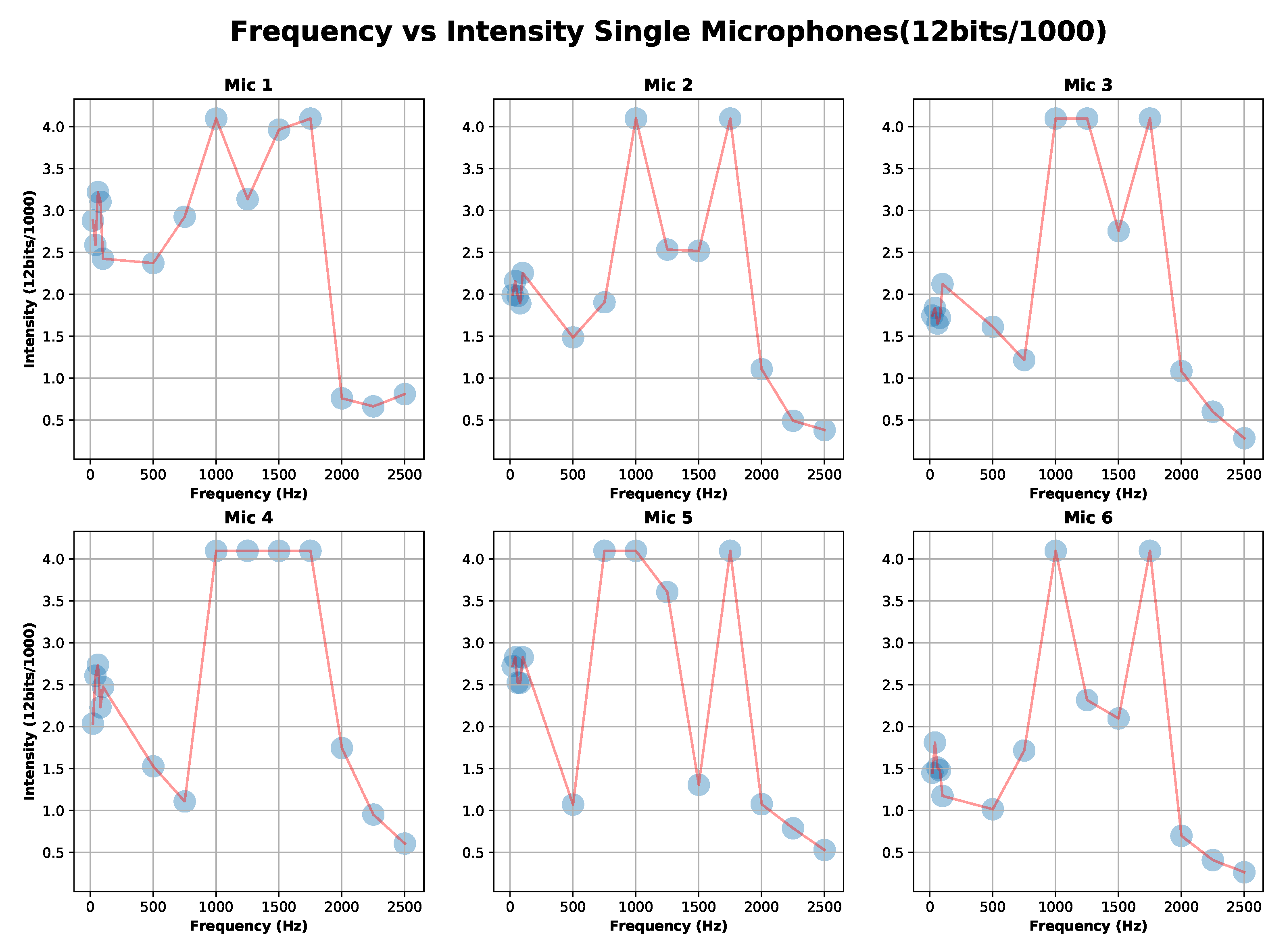
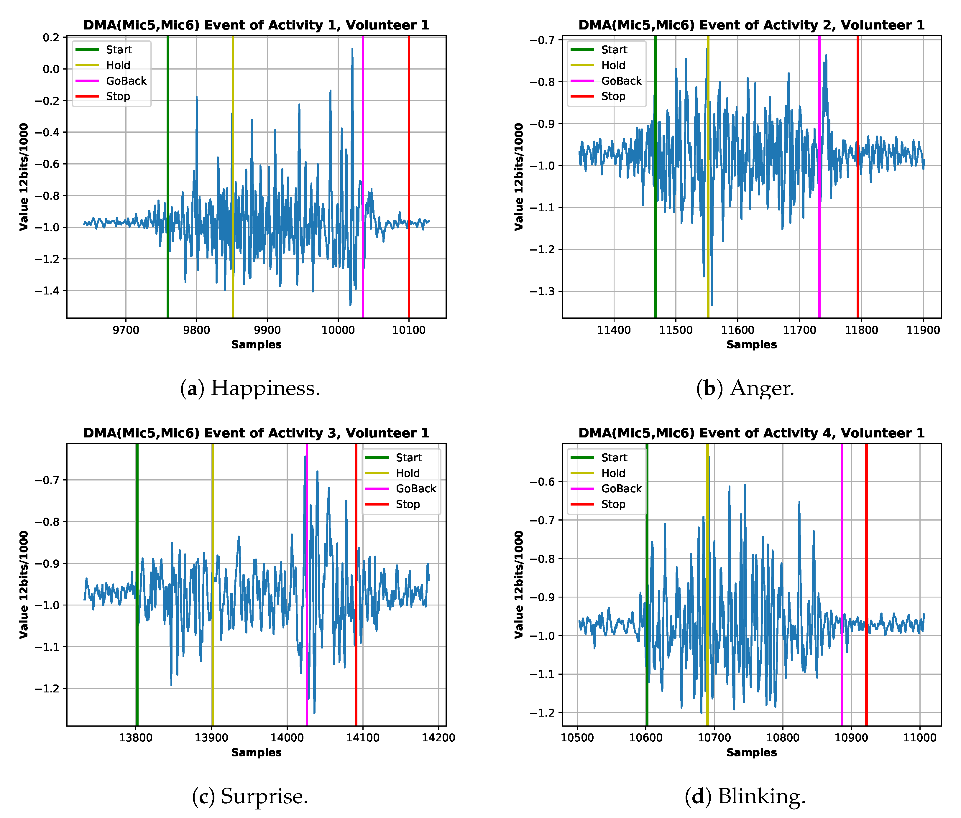

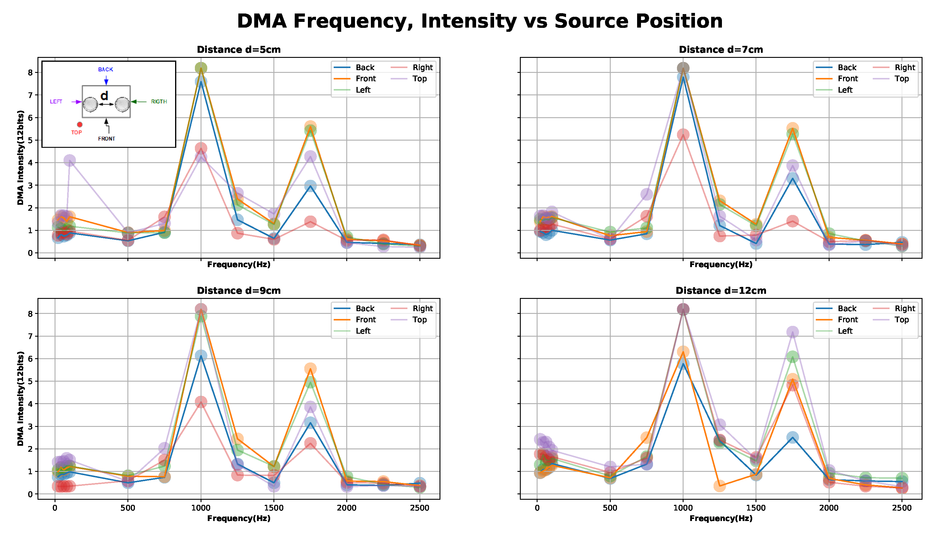
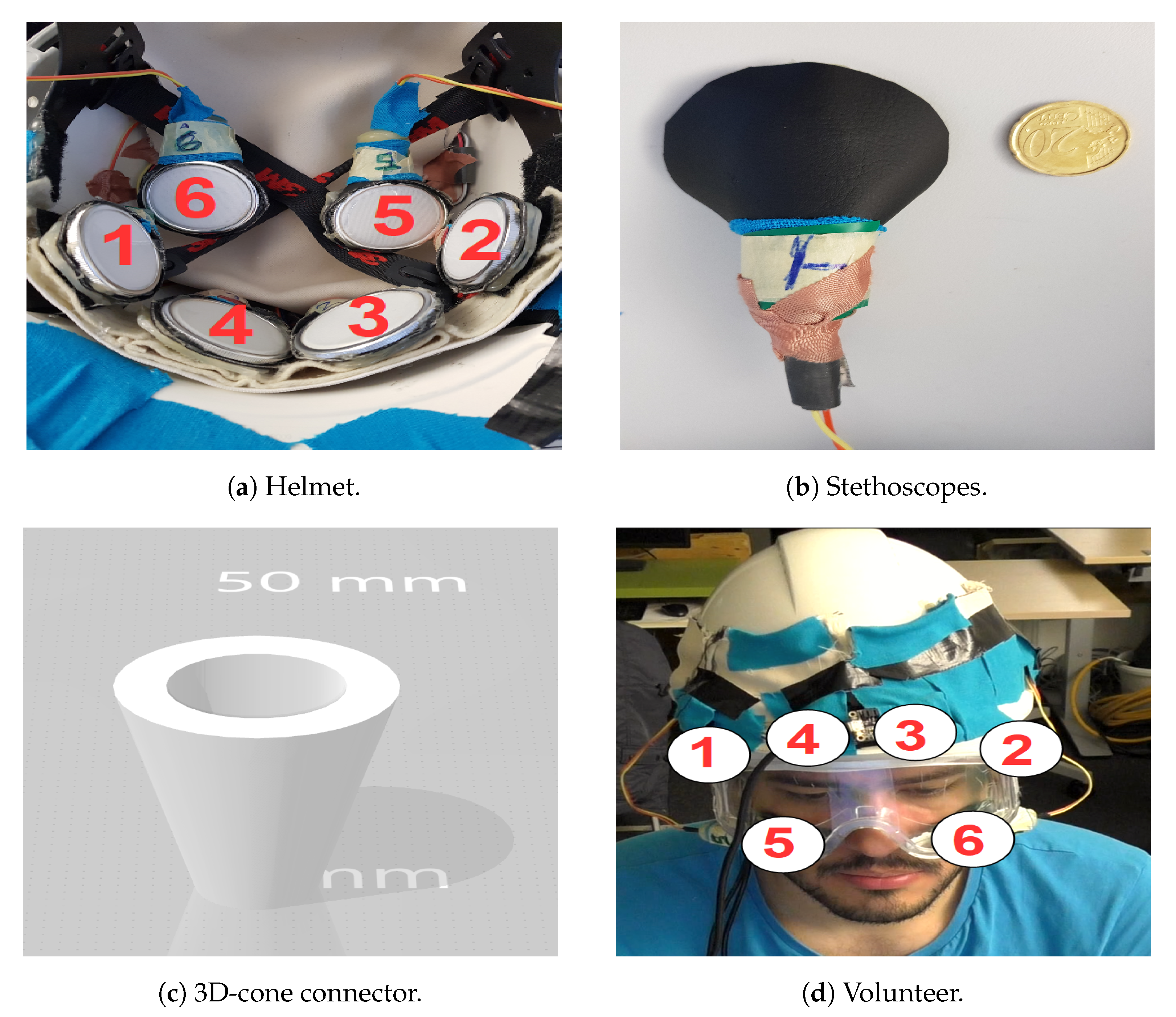

| Mic_1 | Mic_2 | Mic_3 | Mic_4 | Mic_5 | Mic_6 |
|---|---|---|---|---|---|
| min = 2.372 | min = 1.486 | min = 1.217 | min = 1.108 | min = 1.071 | min = 1.015 |
| max = 3.219 | max = 2.254 | max = 2.122 | max = 2.737 | max = 4.095 | max = 1.811 |
| mean = 2.787 | mean = 1.953 | mean = 1.701 | mean = 2.103 | mean = 2.656 | mean = 1.451 |
| Study | Description | Participants, Experiment Repetitions and Samples(HPP-REP) | Location | Expressions | Performance |
|---|---|---|---|---|---|
| Our Approach | Sthetoscope DMAs. | 8-3 with time gap. [2400 + 240 (Neutral)] Samples. | Eyebrows (LOC1), Cheeks (LOC2) and Temples (LOC3). | Happiness, anger, surprise, sadness, upset and disgusted, and gestures as kissing, winkling, sticking the tongue out, taking a pill and neutral. Total = 11. | ** User-dependent = 60–89% f1. * User-independent (LOC1 and LOC2) = 53% f1, ** User-independent (LOC2 and LOC3) = 49% f1. |
| Photo Reflective [12] | 17 Photo sensors. | ** Case A: 8-1 without time gap. 960 Samples (8 expressions X 15 poses per volunteer). * Case B: 3-3 different days. 24 Samples (8 expression X 1 pose per volunteer). | Glasses Frame. | Neutral, happy, disgust, angry, surprise, fear, sad, contempt. Total = 8. | ** Case A: User-dependent = 84.8–99.2% accuracy. (50% Training). * User-independent with leave-volunteer out = 48% accuracy. ** Case B: User-dependent with leave-session out (3 volunteers) = 78.1% accuracy. |
| TPM [17] | Textile Pressure Sensors. | 20-5 with time gap. 6000 Samples. | Forehead. | Joy, surprise, sadness, neutral, fear, disgust, anger. Total = 7. | ** User-independent = 38% accuracy (Five-fold cross validation). |
| EMG Gruebler [14] | 3 Electrode pairs. | 10-1. 160 Samples (4 repetitions for each expressions). | Temples. | Neutral, smiling, frowning, and neither (biting and neutral). Total = 4 | ** User-dependent => 80% accuracy for Smiling and Frowning (training = 3 repetitions per expression) |
| EMG Perusquia [15] | Four surface EMG channels. | 23-1. 238 smiles, 32 micro-smiles and total of 421 expressions. | Temples. | Micro-smile, no-expression, smile, and laughter. Total = 4 | ** User-dependent => 90% accuracy. |
© 2020 by the authors. Licensee MDPI, Basel, Switzerland. This article is an open access article distributed under the terms and conditions of the Creative Commons Attribution (CC BY) license (http://creativecommons.org/licenses/by/4.0/).
Share and Cite
Bello, H.; Zhou, B.; Lukowicz, P. Facial Muscle Activity Recognition with Reconfigurable Differential Stethoscope-Microphones. Sensors 2020, 20, 4904. https://doi.org/10.3390/s20174904
Bello H, Zhou B, Lukowicz P. Facial Muscle Activity Recognition with Reconfigurable Differential Stethoscope-Microphones. Sensors. 2020; 20(17):4904. https://doi.org/10.3390/s20174904
Chicago/Turabian StyleBello, Hymalai, Bo Zhou, and Paul Lukowicz. 2020. "Facial Muscle Activity Recognition with Reconfigurable Differential Stethoscope-Microphones" Sensors 20, no. 17: 4904. https://doi.org/10.3390/s20174904
APA StyleBello, H., Zhou, B., & Lukowicz, P. (2020). Facial Muscle Activity Recognition with Reconfigurable Differential Stethoscope-Microphones. Sensors, 20(17), 4904. https://doi.org/10.3390/s20174904


