Evaluation of Hemodialysis Arteriovenous Bruit by Deep Learning

 ,
,
Abstract
1. Introduction
2. Materials and Methods
2.1. Participants
2.2. Methods
2.2.1. Data Preprocessing: Extraction of Single Beat of the Arteriovenous Fistula Sound
2.2.2. Data Analysis
3. Results
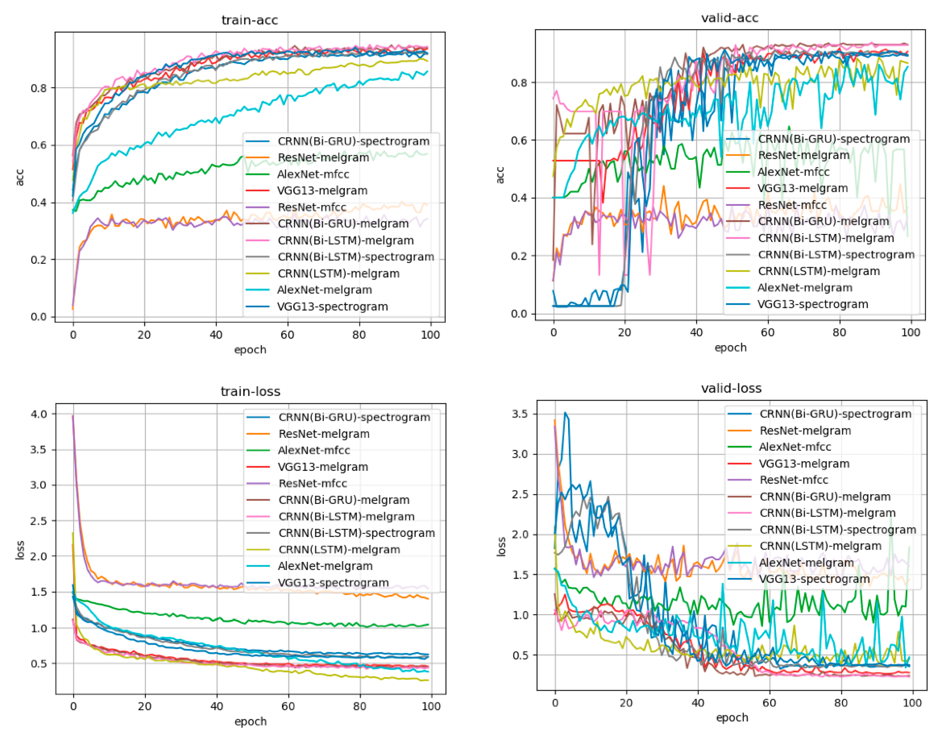
3.1. Learning Curve
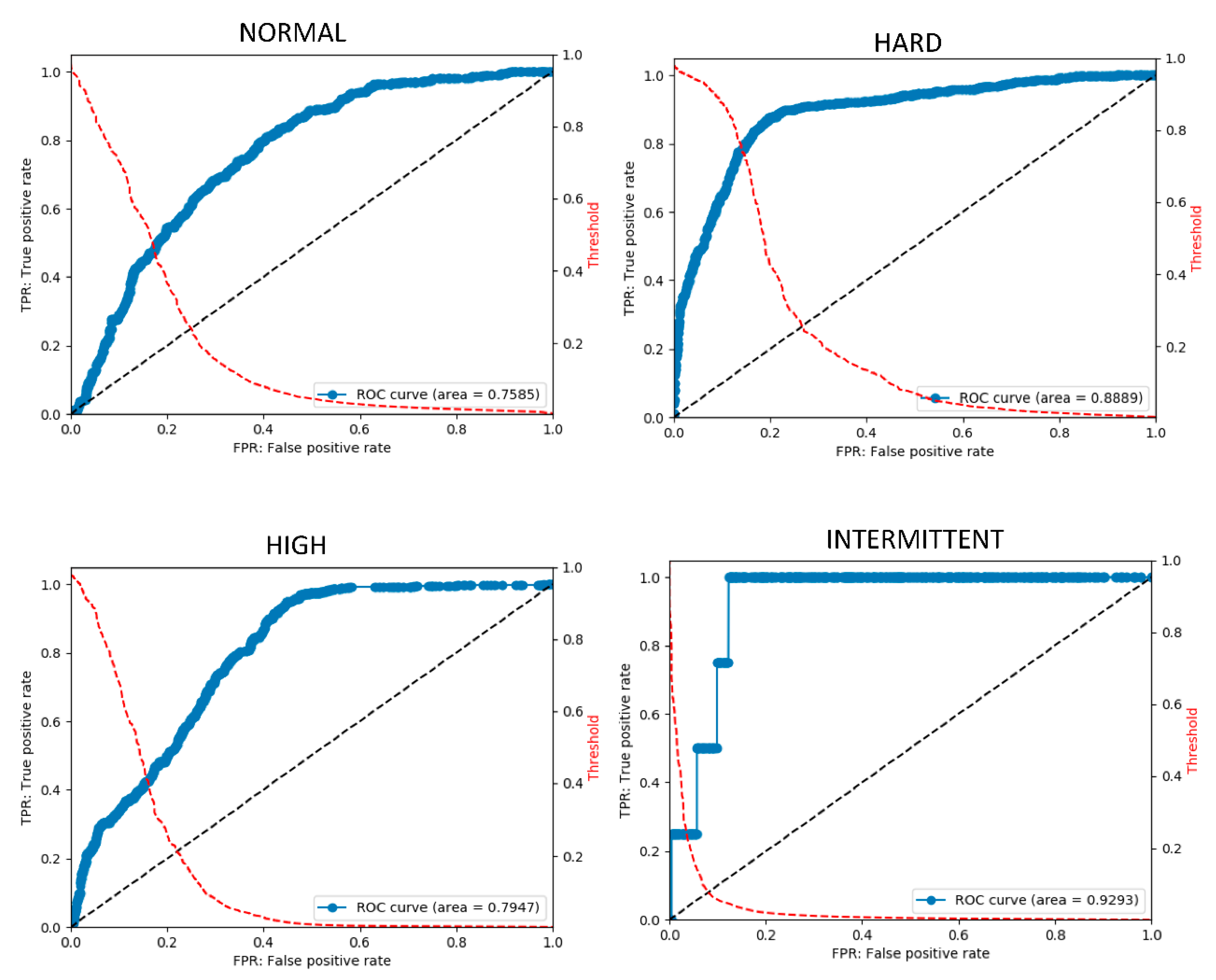
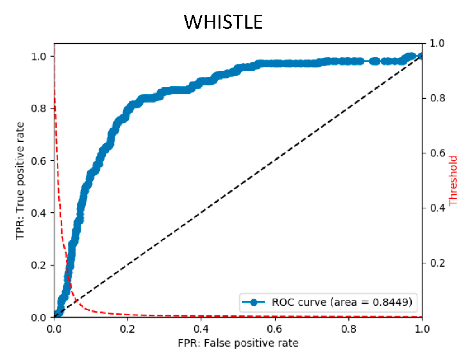
3.2. Postprocessing
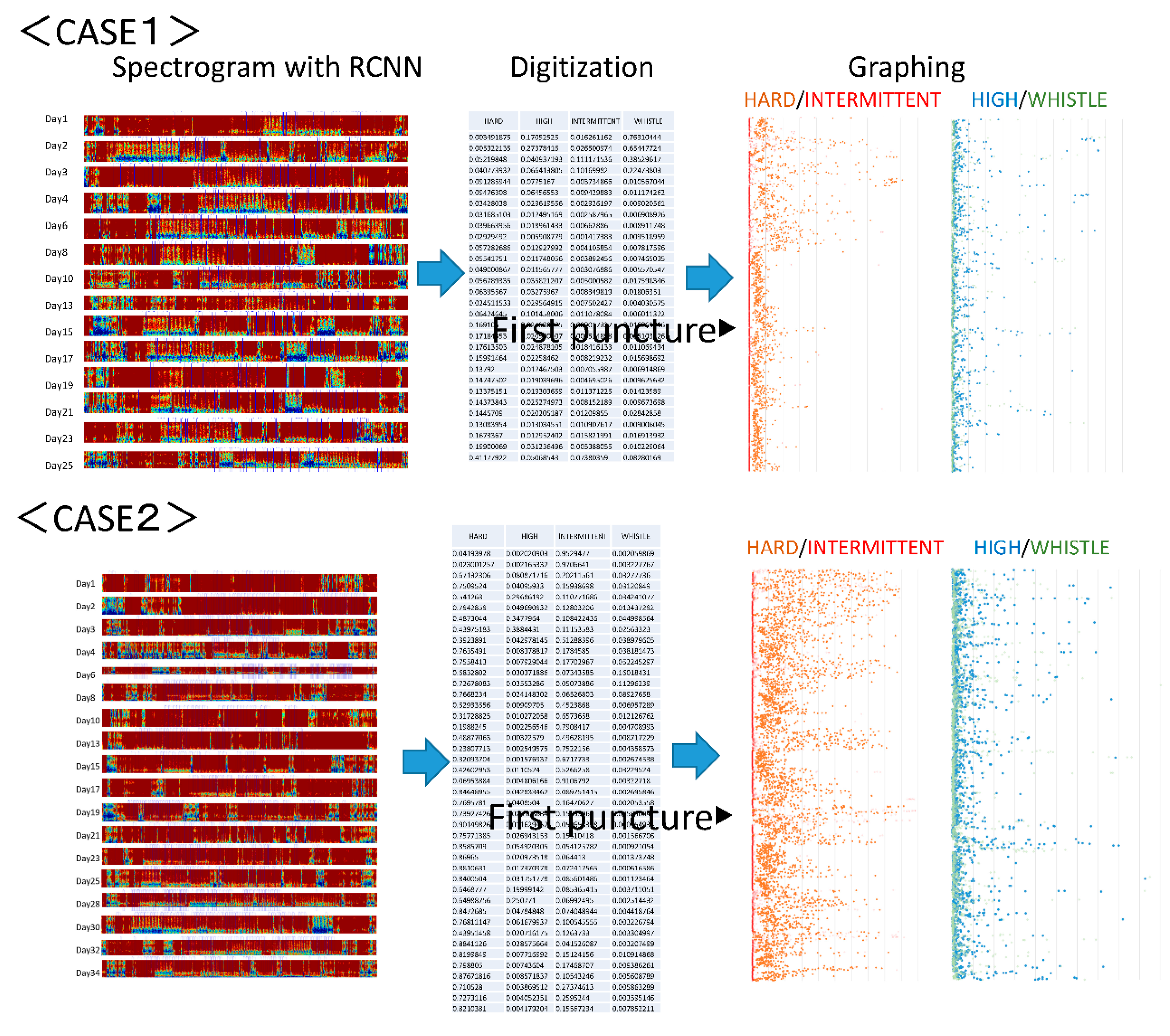
3.3. Clinical Application
4. Discussion
5. Conclusions
Author Contributions
Funding
Acknowledgments
Conflicts of Interest
References
- Lee, T.; Barker, J.; Allon, M. Needle Infiltration of Arteriovenous Fistulae in Hemodialysis: Risk Factors and Consequences. Am. J. Kidney Dis. 2006, 47, 1020–1026. [Google Scholar] [CrossRef] [PubMed]
- Remuzzi, A.; Ene-Iordache, B. Novel Paradigms for Dialysis Vascular Access: Upstream Hemodynamics and Vascular Remodeling in Dialysis Access Stenosis. Clin. J. Am. Soc. Nephrol. 2013, 8, 2186–2193. [Google Scholar] [CrossRef] [PubMed]
- Brahmbhatt, A.; Remuzzi, A.; Franzoni, M.; Misra, S. The molecular mechanisms of hemodialysis vascular access failure. Kidney Int. 2016, 89, 303–316. [Google Scholar] [CrossRef]
- Badero, O.J.; Salifu, M.O.; Wasse, H.; Work, J. Frequency of Swing-Segment Stenosis in Referred Dialysis Patients With Angiographically Documented Lesions. Am. J. Kidney Dis. 2008, 51, 93–98. [Google Scholar] [CrossRef] [PubMed]
- Schmidli, J.; Widmer, M.K.; Basile, C.; De Donato, G.; Gallieni, M.; Gibbons, C.P.; Haage, P.; Hamilton, G.; Hedin, U.; Kamper, L.; et al. Editor’s Choice—Vascular Access: 2018 Clinical Practice Guidelines of the European Society for Vascular Surgery (ESVS). Eur. J. Vasc. Endovasc. Surg. 2018, 55, 757–818. [Google Scholar] [CrossRef]
- Vascular Access 2006 Work Group. National Kidney Foundation Vascular Access 2006 Work Group. KDOQI. Clinical practice guidelines for vascular access. Am. J. Kidney Dis. 2006, 48 (Suppl. 1), S176–S247. [Google Scholar]
- Al-Jaishi, A.A.; Oliver, M.J.; Thomas, S.M.; Lok, C.E.; Zhang, J.C.; Garg, A.X.; Kosa, S.D.; Quinn, R.R.; Moist, L.M. Patency Rates of the Arteriovenous Fistula for Hemodialysis: A Systematic Review and Meta-analysis. Am. J. Kidney Dis. 2014, 63, 464–478. [Google Scholar] [CrossRef]
- Salman, L.; Beathard, G. Interventional Nephrology: Physical Examination as a Tool for Surveillance for the Hemodialysis Arteriovenous Access. Clin. J. Am. Soc. Nephrol. 2013, 8, 1220–1227. [Google Scholar] [CrossRef]
- Sato, T. New diagnostic method according to the acoustic analysis of the shunt blood vessel noise. Toin Univ. Yokohama Eng. Jpn. Soc. Dial. Ther. J. 2005, 2, 332–341. [Google Scholar]
- Kokorozashi, N. Analysis of the shunt sound frequency characteristic changes associated with shunt stenosis. Jpn. Soc. Dial. Ther. J. 2010, 3, 287–295. [Google Scholar]
- Todo, A.; Kadonaka, T.; Yoshioka, M.; Ueno, A.; Mitani, M.; Katsurao, H. Frequency Analysis of Shunt Sounds in the Arteriovenous Fistula on Hemodialysis Patients. In Proceedings of the 6th International Conference on Soft Computing and Intelligent Systems, and the 13th International Symposium on Advanced Intelligence Systems, Kobe, Japan, 20–24 November 2012. [Google Scholar] [CrossRef]
- Wang, H.-Y.; Wu, C.-H.; Chen, C.-Y.; Lin, B.-S. Novel Noninvasive Approach for Detecting Arteriovenous Fistula Stenosis. IEEE Trans. Biomed. Eng. 2014, 61, 1851–1857. [Google Scholar] [CrossRef] [PubMed]
- Kamijo, Y.; Kanda, E.; Horiuchi, H.; Kounoue, N.; Ono, K.; Maeda, K.; Yanai, A.; Honda, K.; Tsujimoto, R.; Yanagi, M.; et al. Continuous monitoring of blood pressure by analyzing the blood flow sound of arteriovenous fistula in hemodialysis patients. Clin. Exp. Nephrol. 2017, 22, 677–683. [Google Scholar] [CrossRef] [PubMed]
- Serven, D.; Brummit, C. pyGAM: Generalized Additive Models in Python. 2018. Available online: https://zenodo.org/record/1476122 (accessed on 26 August 2020).
- Iqbal, T.; Kong, Q.; Plumbley, M.D.; Wang, W. Stacked Convolutional Neural Networks for General-Purpose Audio Tagging; University of Surrey: Guildford, UK, 2018. [Google Scholar]
- Owada, A.; Saito, H.; Mochizuki, T.; Tanaka, M.; Otsuka, M.; Yokoyama, Y.; Fukuda, S. Radial Arterial Spasm in Uremic Patients Undergoing Construction of Arteriovenous Hemodialγsis Fistulas: Diagnosis and Prophylaxis with Intravenous Nicardipine. Nephron 1993, 64, 501–504. [Google Scholar] [CrossRef] [PubMed]
- Keisuke, O. Cannulation should be more than 3 weeks after creation of a radial-cephalic arterio-venous fistula. Clin. Surg. 2019, 4, 2299. [Google Scholar]
- Litjens, G.; Kooi, T.; Bejnordi, B.E.; Setio, A.A.A.; Ciompi, F.; Ghafoorian, M.; Van Der Laak, J.A.; Van Ginneken, B.; Sánchez, C.I. A survey on deep learning in medical image analysis. Med. Image Anal. 2017, 42, 60–88. [Google Scholar] [CrossRef]
- Akatsuka, J.; Yamamoto, Y.; Sekine, T.; Numata, Y.; Morikawa, H.; Tsutsumi, K.; Yanagi, M.; Endo, Y.; Takeda, H.; Hayashi, T.; et al. Illuminating Clues of Cancer Buried in Prostate MR Image: Deep Learning and Expert Approaches. Biomolecules 2019, 9, 673. [Google Scholar] [CrossRef]
- Asif, T.; Mohiuddin, A.; Hasan, B.; Pauly, R.R. Importance of Thorough Physical Examination: A Lost Art. Cureus 2017, 9, 1212. [Google Scholar] [CrossRef]
- Esteva, A.; Kuprel, B.; Novoa, R.A.; Ko, J.; Swetter, S.M.; Blau, H.M.; Thrun, S. Dermatologist-level classification of skin cancer with deep neural networks. Nature 2017, 542, 115–118. [Google Scholar] [CrossRef]
- Messner, E.; Zöhrer, M.; Pernkopf, F. Heart Sound Segmentation—An Event Detection Approach Using Deep Recurrent Neural Networks. IEEE Trans. Biomed. Eng. 2018, 65, 1964–1974. [Google Scholar] [CrossRef]
- Raza, A.; Mehmood, A.; Ullah, S.; Ahmad, M.; Choi, G.S.; On, B.-W. Heartbeat Sound Signal Classification Using Deep Learning. Sensors 2019, 19, 4819. [Google Scholar] [CrossRef]
- Selvaraju, R.R.; Cogswell, M.; Das, A.; Vedantam, R.; Parikh, D.; Batra, D. Grad-CAM: Visual Explanations from Deep Networks via Gradient-Based Localization. Int. J. Comput. Vis. 2020, 128, 336–359. [Google Scholar] [CrossRef]
- Wakisaka, Y.; Miura, T. A new method for estimating blood flow through arteriovenous fistulas and grafts in patients undergoing hemodialysis. Jpn. Soc. Dial. Ther. 2019, 52, 569–575. [Google Scholar] [CrossRef]
- Higashi, D.; Nishijima, K. Classification of Shunt Murmurs for Diagnosis of Arteriovenous Fistula Stenosis. In Proceedings of the 2018 Asia-Pacific Signal and Information Processing Association Annual Summit and Conference (APSIPA ASC), Honolulu, HI, USA, 12–15 November 2018. [Google Scholar] [CrossRef]
- Chalapathy, R.; Chawla, S. Deep learning for anomaly detection: A survey. arXiv 2019, arXiv:1901.03407. [Google Scholar]
- Vununu, C.; Moon, K.-S.; Lee, S.-H.; Kwon, K.-R. A Deep Feature Learning Method for Drill Bits Monitoring Using the Spectral Analysis of the Acoustic Signals. Sensors 2018, 18, 2634. [Google Scholar] [CrossRef]
- Heo, S.-J.; Kim, Y.; Yun, S.; Lim, S.-S.; Kim, J.; Nam, C.M.; Park, E.-C.; Jung, I.; Yoon, J.-H. Deep Learning Algorithms with Demographic Information Help to Detect Tuberculosis in Chest Radiographs in Annual Workers’ Health Examination Data. Int. J. Environ. Res. Public Health 2019, 16, 250. [Google Scholar] [CrossRef]
- Matsuura, K.; Gotoh, Y.; Sadaoka, S.; Takase, K.; Narimatsu, Y. Guidelines for basic techniques in vascular access intervention therapy (VAIVT). Interv. Radiol. 2018, 3, 28–43. [Google Scholar] [CrossRef]
- Murakami, K.; Inomata, F.; Takeda, T.; Utino, J.; Sakai, T.; Kouno, T.; Sigematu, T.; Yoshida, T. Usefulness of pulsed doppler ultrasonography to manage internal AV shunt. Kidney Dial. 2003, 55, 39–43. [Google Scholar]


| Characteristic | Value | |
|---|---|---|
| Age (median (IQR), years) | 73 (63–79) | |
| Gender (n) | Male | 13 |
| Female | 7 | |
| Dialysis duration (median (IQR), years) | 0.01 (0–19) | |
| Cause of end-stage renal disease | ||
| Diabetes | 11 | |
| Glomerulonephritis | 5 | |
| Others | 4 | |
| Type of arteriovenous fistula | ||
| Radiocephalic AVF at front arm | 17 | |
| Radiocephalic AVF at mid forearm | 2 | |
| Brachiocephalic AVF at elbow | 1 | |
| Training | Test | Total | |
|---|---|---|---|
| Normal | 394 | 485 | 879 |
| Hard | 578 | 901 | 1479 |
| High | 670 | 563 | 1233 |
| Intermittent | 91 | 4 | 95 |
| Whistle | 91 | 217 | 308 |
| Total | 1824 | 2170 | 3994 |
| VGG13 | CRNN (Bi-GRU) | CRNN (Bi-LSTM) |
|---|---|---|
| Log mel spectrogram | Log mel spectrogram | Log mel spectrogram |
| 3 × 3, 64, BN, ReLU | 3 × 3, 64, BN, ReLU | 3 × 3, 64, BN, ReLU |
| 3 × 3, 64, BN, ReLU | 3 × 3, 64, BN, ReLU | 3 × 3, 64, BN, ReLU |
| 2 × 2 Max Pooling | 2 × 2 Max Pooling | 2 × 2 Max Pooling |
| 3 × 3128, BN, ReLU | 3 × 3128, BN, ReLU | 3 × 3128, BN, ReLU |
| 3 × 3128, BN, ReLU | 3 × 3128, BN, ReLU | 3 × 3128, BN, ReLU |
| 2 × 2 Max Pooling | 2 × 2 Max Pooling | 2 × 2 Max Pooling |
| 3 × 3256, BN, ReLU | 3 × 3256, BN, ReLU | 3 × 3256, BN, ReLU |
| 3 × 3256, BN, ReLU | 3 × 3256, BN, ReLU | 3 × 3256, BN, ReLU |
| 2 × 2 Max Pooling | 2 × 2 Max Pooling | 2 × 2 Max Pooling |
| 3 × 3512, BN, ReLU | 3 × 3512, BN, ReLU | 3 × 3512, BN, ReLU |
| 3 × 3512, BN, ReLU | 3 × 3512, BN, ReLU | 3 × 3512, BN, ReLU |
| 2 × 2 Max Pooling | 2 × 2 Max Pooling | 2 × 2 Max Pooling |
| 3 × 3512, BN, ReLU | 3 × 3512, BN, ReLU | 3 × 3512, BN, ReLU |
| 3 × 3512, BN, ReLU | 3 × 3512, BN, ReLU | 3 × 3512, BN, ReLU |
| Bi-GRU, 512, ReLU | Bi-LSTM, 512, ReLU | |
| Global average pooling | ||
| Softmax (5 classes) | ||
| Feature | 64 | 128 | 256 | 512 | 1024 | ||||||||||
|---|---|---|---|---|---|---|---|---|---|---|---|---|---|---|---|
| CNN | GRU | LSTM | CNN | GRU | LSTM | CNN | GRU | LSTM | CNN | GRU | LSTM | CNN | GRU | LSTM | |
| Normal | 0.58 | 0.59 | 0.60 | 0.70 | 0.72 | 0.64 | 0.69 | 0.73 | 0.66 | 0.69 | 0.72 | 0.66 | 0.70 | 0.72 | 0.65 |
| Hard | 0.70 | 0.70 | 0.68 | 0.81 | 0.81 | 0.69 | 0.84 | 0.87 | 0.78 | 0.83 | 0.90 | 0.85 | 0.83 | 0.91 | 0.73 |
| High | 0.77 | 0.77 | 0.76 | 0.80 | 0.77 | 0.78 | 0.80 | 0.80 | 0.80 | 0.78 | 0.80 | 0.80 | 0.79 | 0.76 | 0.77 |
| Intermittent | 0.83 | 0.88 | 0.77 | 0.78 | 0.85 | 0.82 | 0.83 | 0.78 | 0.77 | 0.87 | 0.87 | 0.82 | 0.84 | 0.94 | 0.92 |
| Whistle | 0.89 | 0.85 | 0.85 | 0.89 | 0.89 | 0.86 | 0.89 | 0.89 | 0.89 | 0.87 | 0.87 | 0.87 | 0.88 | 0.88 | 0.86 |
| NORMAL | HARD | HIGH | INTERMITTENT | WHISTLE | MEAN | |
|---|---|---|---|---|---|---|
| accuracy | 0.753 | 0.833 | 0.729 | 0.935 | 0.855 | 0.821 |
| precision | 0.45 | 0.766 | 0.478 | 0.014 | 0.36 | 0.414 |
| recall | 0.468 | 0.862 | 0.478 | 0.5 | 0.581 | 0.578 |
| specificity | 0.836 | 0.812 | 0.817 | 0.936 | 0.885 | 0.857 |
| f1 | 0.459 | 0.811 | 0.478 | 0.028 | 0.444 | 0.444 |
| AUC | 0.759 | 0.889 | 0.795 | 0.929 | 0.845 | 0.843 |
© 2020 by the authors. Licensee MDPI, Basel, Switzerland. This article is an open access article distributed under the terms and conditions of the Creative Commons Attribution (CC BY) license (http://creativecommons.org/licenses/by/4.0/).
Share and Cite
Ota, K.; Nishiura, Y.; Ishihara, S.; Adachi, H.; Yamamoto, T.; Hamano, T. Evaluation of Hemodialysis Arteriovenous Bruit by Deep Learning. Sensors 2020, 20, 4852. https://doi.org/10.3390/s20174852
Ota K, Nishiura Y, Ishihara S, Adachi H, Yamamoto T, Hamano T. Evaluation of Hemodialysis Arteriovenous Bruit by Deep Learning. Sensors. 2020; 20(17):4852. https://doi.org/10.3390/s20174852
Chicago/Turabian StyleOta, Keisuke, Yousuke Nishiura, Saki Ishihara, Hihoko Adachi, Takehisa Yamamoto, and Takayuki Hamano. 2020. "Evaluation of Hemodialysis Arteriovenous Bruit by Deep Learning" Sensors 20, no. 17: 4852. https://doi.org/10.3390/s20174852
APA StyleOta, K., Nishiura, Y., Ishihara, S., Adachi, H., Yamamoto, T., & Hamano, T. (2020). Evaluation of Hemodialysis Arteriovenous Bruit by Deep Learning. Sensors, 20(17), 4852. https://doi.org/10.3390/s20174852