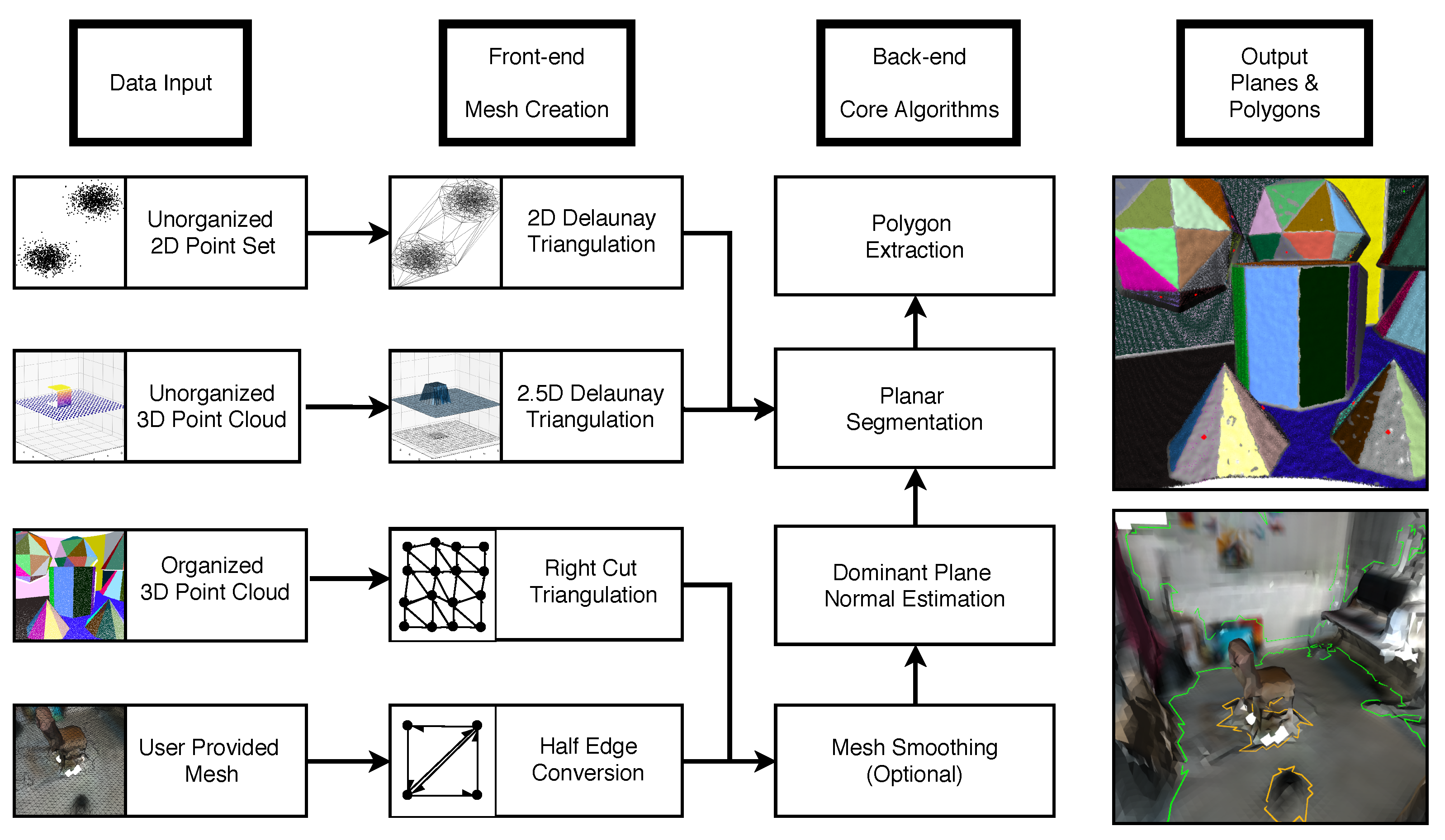
Figure 1.
Overview of Polylidar3D. Input data can be 2D point sets, unorganized/organized 3D point clouds, or user-provided meshes. Polylidar3D’s front-end transforms input data to a half-edge triangulation structure. The back-end is responsible for mesh smoothing, dominant plane normal estimation, planar segmentation, and polygon extraction. Polylidar3D outputs both planes (sets of spatially connected triangles) and corresponding polygonal representations. An example output of color-coded extracted planes from organized point clouds is shown (top right). An example of extracted polygons from a user-provided mesh is shown (bottom right). The green line represents the concave hull; orange lines show interior holes representing obstacles.
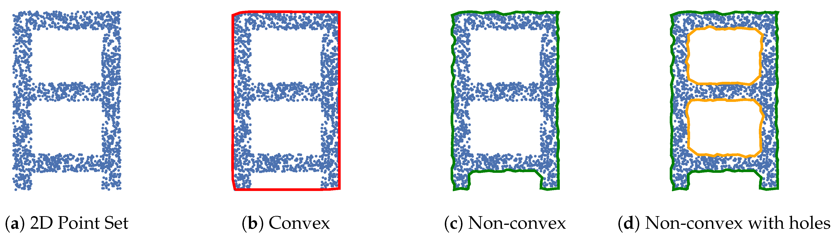
Figure 2.
Example polygons that can be generated from plane segmented point clouds. (a) 2D point set representation of a floor diagram with interior offices; (b) Convex polygon; (c) non-convex polygon; (d) and non-convex polygon with holes. The exterior hull (green) and interior holes (orange) are indicated.
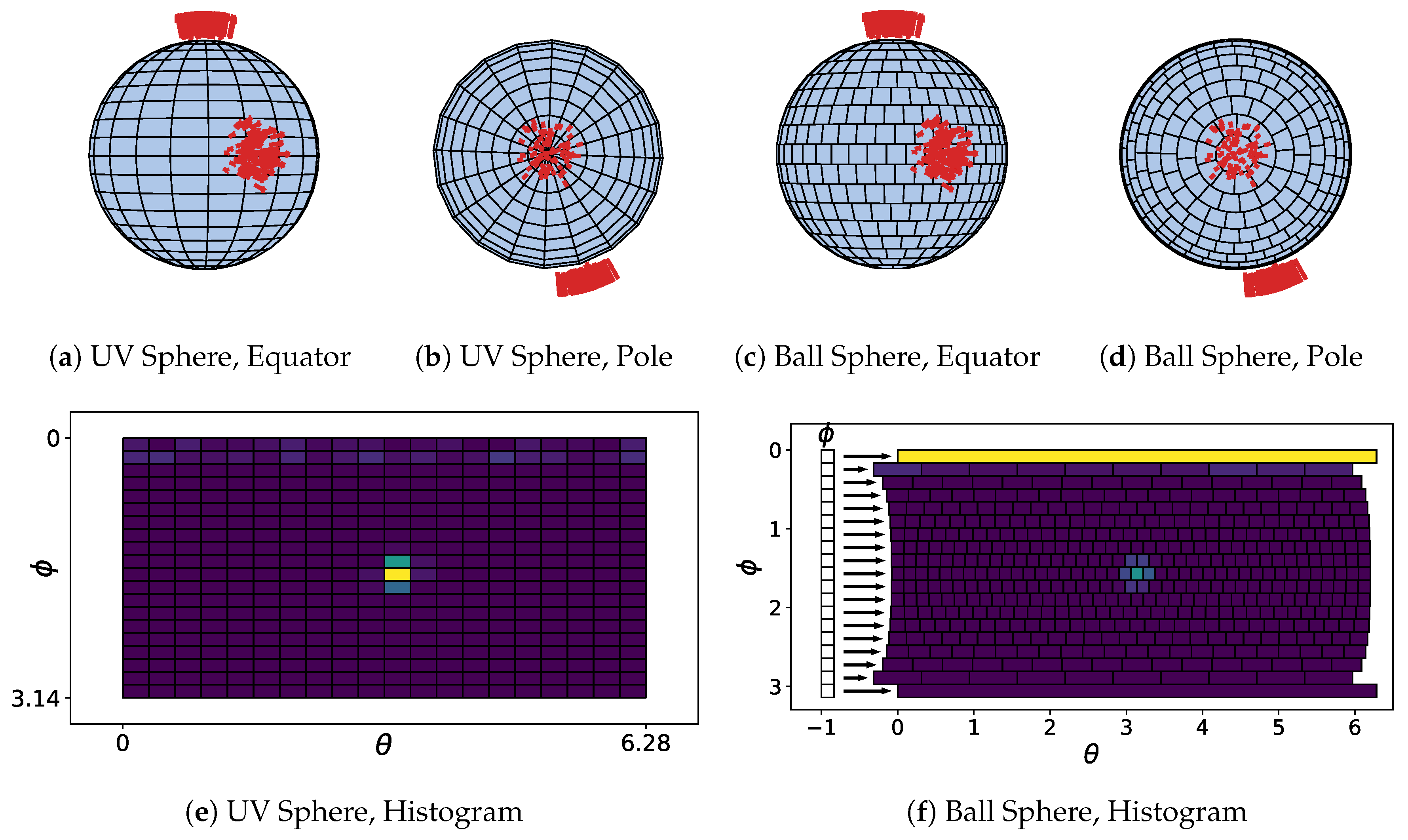
Figure 3.
Examples of integrating normals from two identically “noisy” planes (red arrows, Gaussian distributed) into a UV Sphere (a,b) and Ball Sphere (c,d). Note the anisotropic property of sphere cells caused by unequal area and shape; (e) The UV Sphere histogram is unable to detect the peak at the pole; (f) The Ball sphere is able to detect both peaks, but the north pole cell is significantly larger leading to an incorrectly higher value than the equator cell.
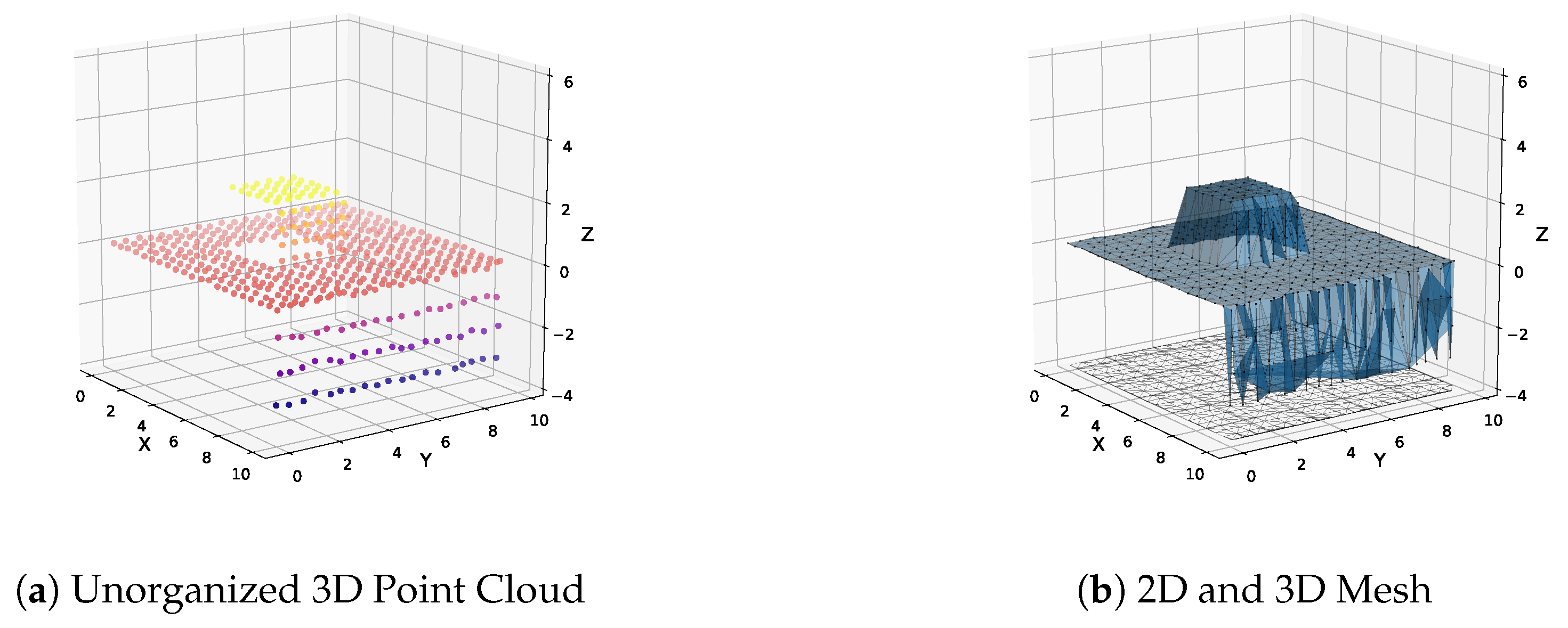
Figure 4.
Example conversion of an unorganized 3D point cloud to a 3D triangular mesh. (a) Synthetic point cloud of a rooftop scene generated from an overhead laser scanner. A single wall is captured because the scanner is slightly angled; (b) The point cloud is projected to the xy plane and triangulated, generating the dual 3D mesh. Only planes aligned with the xy plane can be captured.
Figure 5.
Example conversion of a 7 × 7 Organized Point Cloud (OPC) to a half-edge triangular mesh. Points are represented by circles; red indicates an invalid value (e.g., 0 depth measurement). (a) Implicit mesh of OPC with right cut triangles, . A unique global id GID = 2 · (u · (N − 1) + v) + k is shown inside each triangle; (b) Indexing scheme to define GIDs for triangles in ; (c) Final mesh with triangles created if and only if all vertices are valid. Unique indices into are marked. maps between GIDs in to .
Figure 6.
Example non-manifold meshes that exhibit condition (1) violations. Red vertices specifically show examples where the vertex triangle set is not fully edge-connected. (
a–
c) will extract any missing triangles as holes from the blue triangular segment; (
d) The missing triangles in this mesh also cause condition (1) violations but will not be captured as holes. They cause the green and blue portion of the mesh to not be edge-connected for region growing in
Section 7.1. They will be extracted as two separate segments with no holes in their respective interiors
Figure 7.
Examples of non-manifold meshes where an edge is shared by more than two triangles. This common edge is shared by green and orange triangles. The green triangles form a two-manifold mesh with the blue triangles while the orange triangle(s) do not. The orange triangles in (a,b) have sufficiently different normals such the green triangles half-edges can be easily linked. However all triangles in (c) have nearly equal normals making this impossible.
Figure 8.
Visualization of a triangle’s neighborhood during bilateral filtering of an organized point cloud. Each 2 × 2 point group forms two triangles creating a mesh. Each triangle’s neighbors are defined by the kernel size. For example a kernel size of five includes all blue and red triangles.
Figure 8.
Visualization of a triangle’s neighborhood during bilateral filtering of an organized point cloud. Each 2 × 2 point group forms two triangles creating a mesh. Each triangle’s neighbors are defined by the kernel size. For example a kernel size of five includes all blue and red triangles.
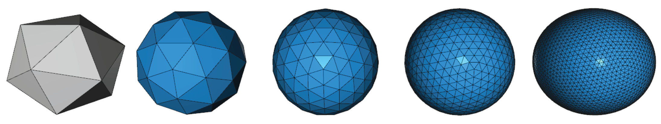
Figure 9.
Approximation of the unit sphere with an icosahedron. The level 0 icosahedron is shown on the left with increasing refinements to the right. Triangle cells become buckets of a histogram on S2.
Figure 9.
Approximation of the unit sphere with an icosahedron. The level 0 icosahedron is shown on the left with increasing refinements to the right. Triangle cells become buckets of a histogram on S2.
Figure 10.
Space filling curve (SFC) of a level 4 icosahedron generated using the S2 Geometry Library. Each cell’s surface normal is mapped to an integer creating a linear ordering for a curve. The curve is colored according to this mapping and traverses each cell.
Figure 10.
Space filling curve (SFC) of a level 4 icosahedron generated using the S2 Geometry Library. Each cell’s surface normal is mapped to an integer creating a linear ordering for a curve. The curve is colored according to this mapping and traverses each cell.
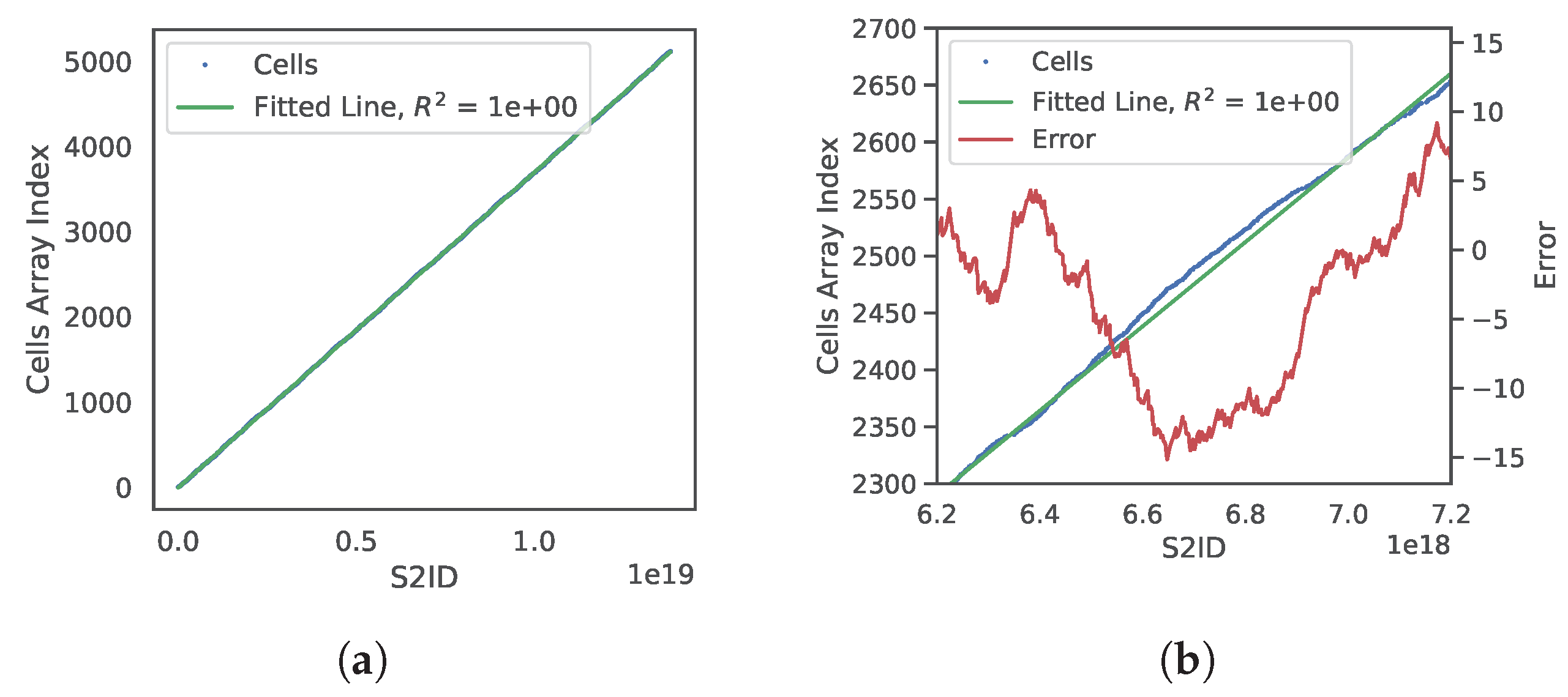
Figure 11.
Linear prediction model for a level four Gaussian Accumulator (GA). The 5120 GA cells are sorted in an array (Cells) by their corresponding spatial index s2id; (a) Plot relating cell s2id and index position in the Cells array with a regressed line (green) to the data; (b) Zoomed-in view showing model error (red line) indicating difference between predicted and actual index for each s2id.
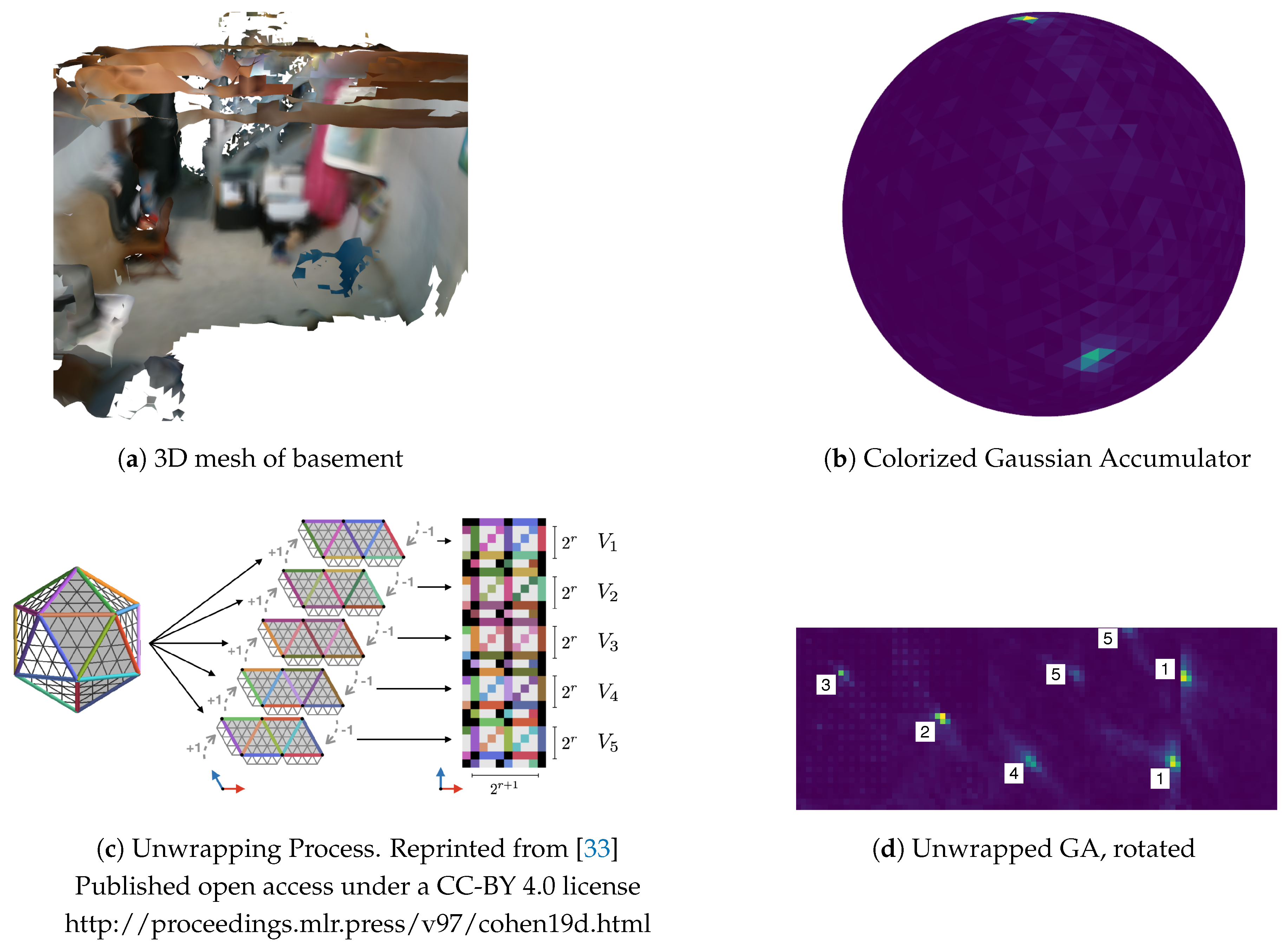
Figure 12.
(
a) Example basement scene mesh; (
b) Mesh triangle normals are integrated into the Gaussian Accumulator and colorized showing peaks for the floor and walls; (
c) Overview of unwrapping a refined icosahedron into a 2D image. Five overlapping charts are stitched together to create a grid. Padding between charts is accomplished by copying adjoining chart neighbors using the unwrapping process and its illustration from [
33]; (
d) Unwrapped Gaussian Accumulator creating a 2D image used for peak detection. White boxes indicate detected peaks. Duplicate peaks are merged (1 & 5) with agglomerative hierarchical clustering.
Figure 13.
(a) An example mesh to demonstrate planar segmentation and polygon extraction using two dominant plane normals, represented by the floor and wall; (b) Every triangle is inspected for filtering and clustered through group assignment. Blue and red triangles meet triangle edge length constraints and are within an angular tolerance of the floor and wall surface normals, respectively; (c) Region growing is performed in parallel for the blue and red triangles. The top chair surface and floor are distinct planar segments; (d) Polygonal representations for each planar segment are shown. The green line represents the concave hull; the orange line depicts any interior holes. Note that small segments and small interior holes are filtered.
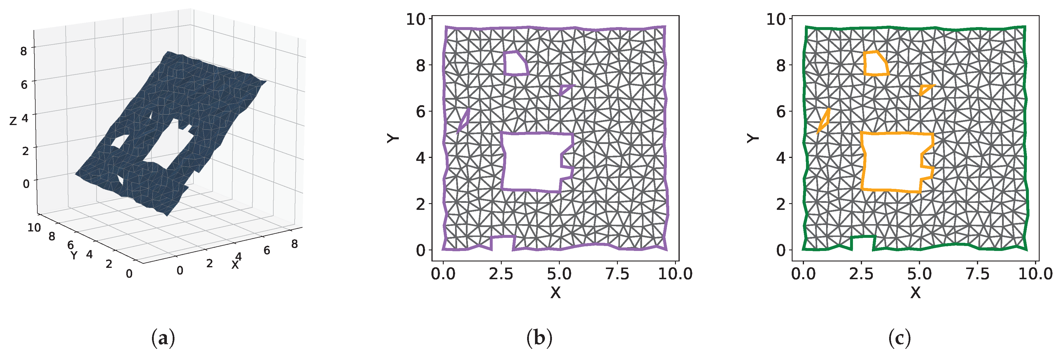
Figure 14.
(a) Example extracted planar triangular segment . Note the four holes in the mesh; (b) Projection of a triangle segment to a geometric plane. Only border edges (purple) are actually needed for projection; (c) A polygon is extracted from border edges with a concave hull (green) and multiple interior holes (orange).
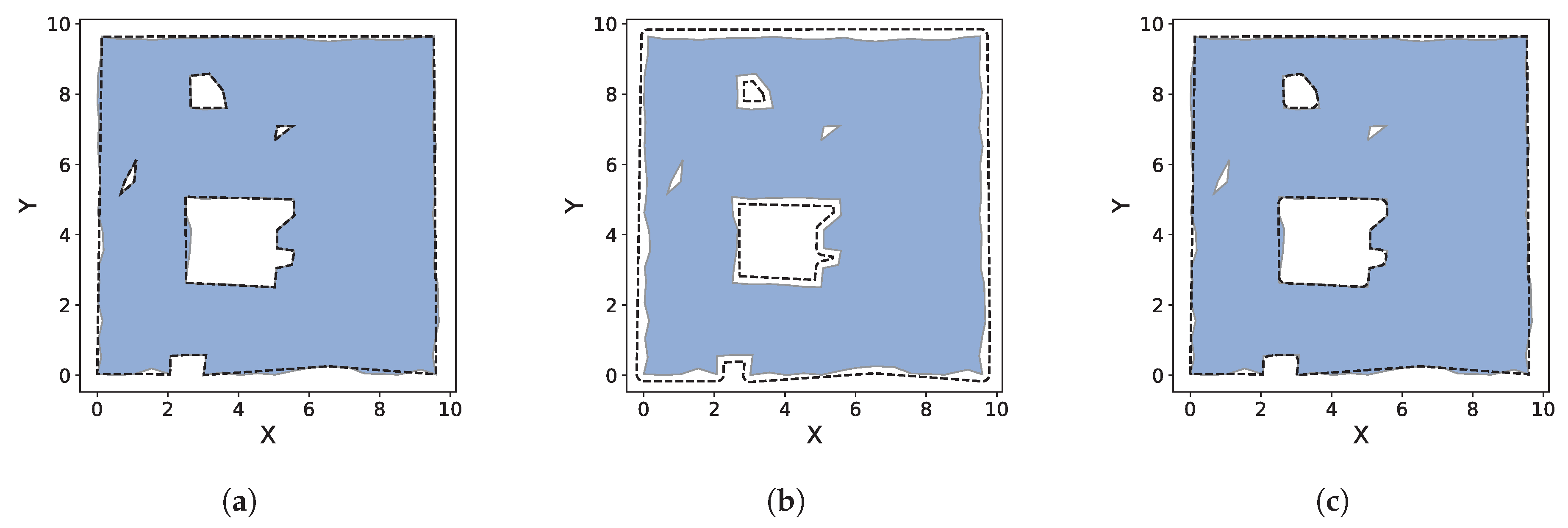
Figure 15.
An example of polygon post processing. The shaded blue polygon is the original polygon extracted (see
Figure 14c). All dashed lines indicate a new polygon generated from a step of post processing. (
a) The polygon is simplified; (
b) The polygon is applied a positive buffer. Two small holes have been “filled” in; (
c) The polygon is applied a negative buffer; only two holes remain.
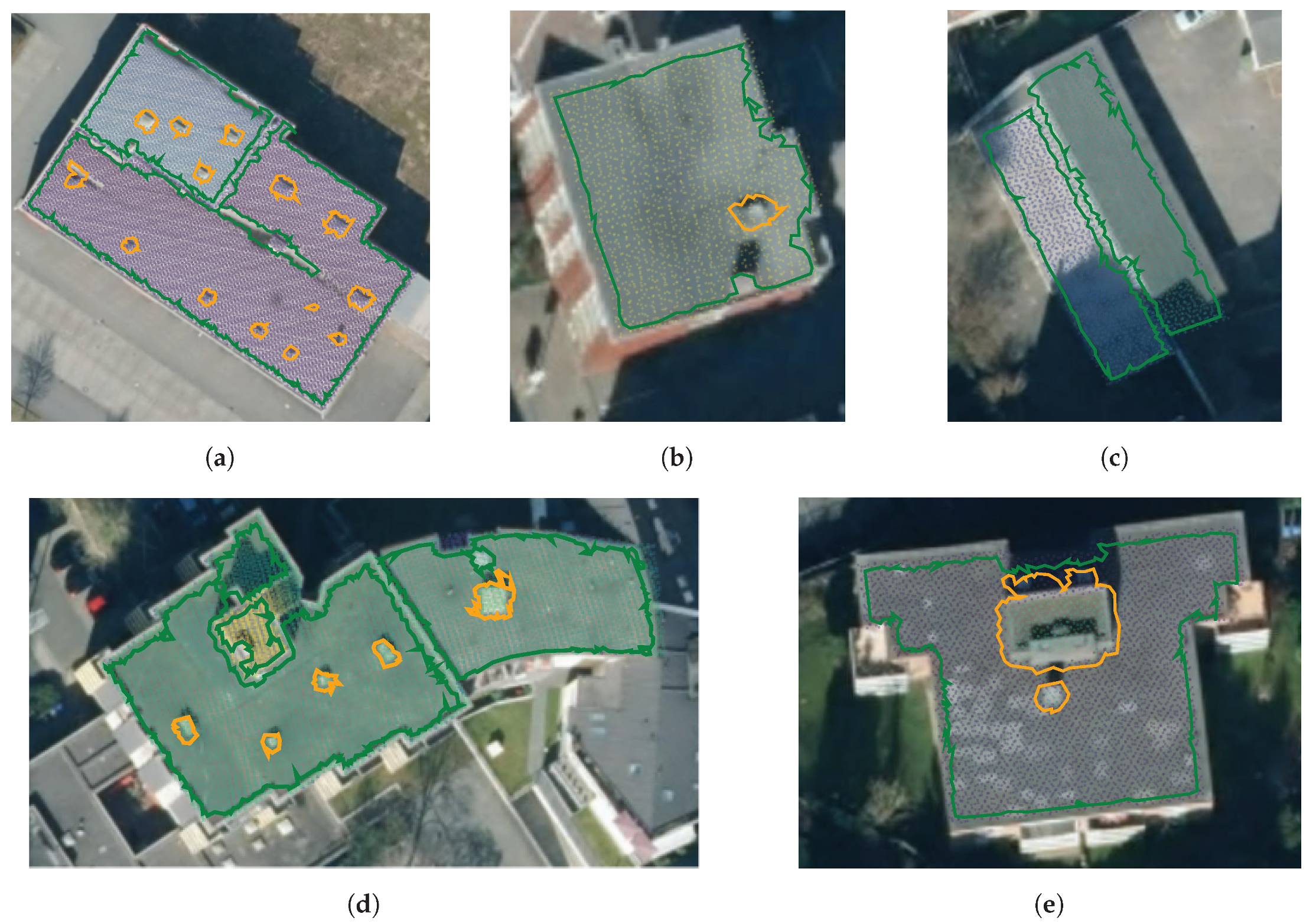
Figure 16.
Polygon extraction of rooftops from unorganized 3D point clouds generated by airborne LiDAR. Each figure (
a–
e) shows the satellite image overlaid with the extracted polygons (green) representing flat surfaces with interior holes (orange) representing obstacles. A colorized point cloud is also overlaid ranging from dark purple to bright yellow denoting a normalized low to high elevation. LiDAR data and satellite images are provided from [
60,
61] respectively, which are from ref. [
62].
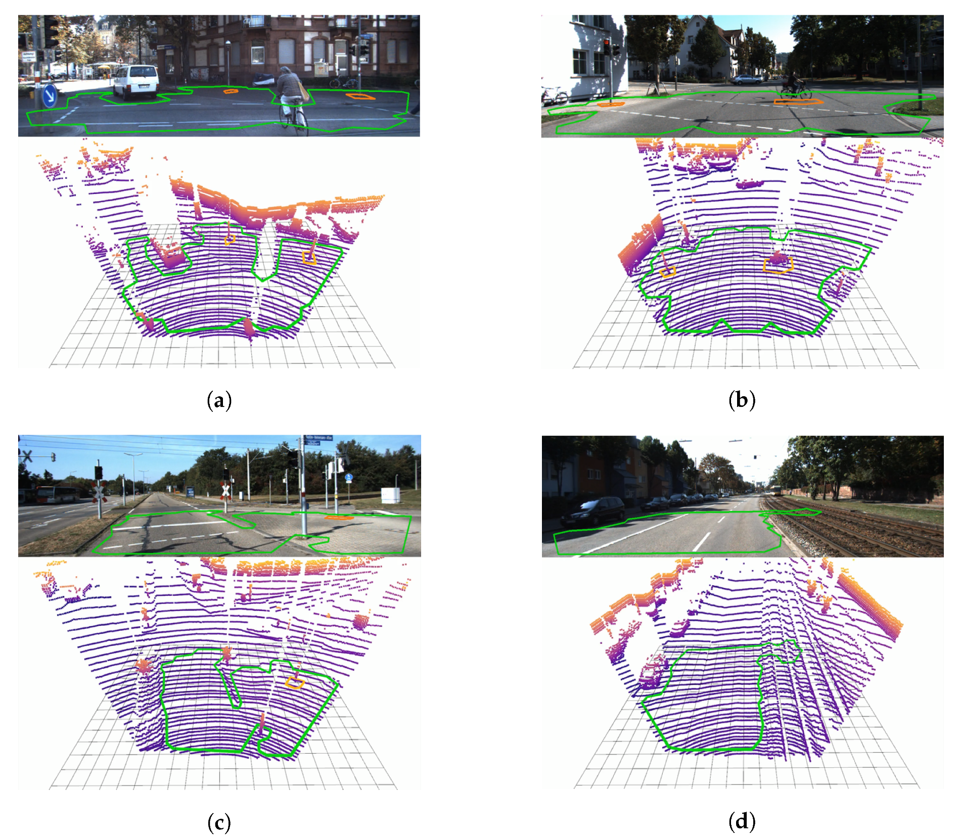
Figure 17.
Polygon extraction from KITTI unorganized 3D point cloud data acquired on a moving vehicle [
63]. Four scenes (
a–
d) are shown, each with two subimages. The top subimage shows polygons projected into the color image while the bottom image shows 3D point cloud and surface polygon(s) from a bird’s eye view. Obstacles on the ground such as the light and signal in (
a) are extracted as (orange) holes.
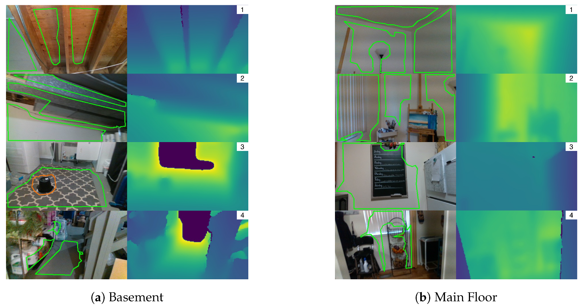
Figure 18.
Real-time polygon extraction from an RGBD camera. Four scenes are shown from the basement (a) and main floor (b) datasets. Color and depth frames are shown side by side for each scene. Polygons are projected onto the color image. Green denotes the exterior hull, and orange denotes any interior holes in the polygon.
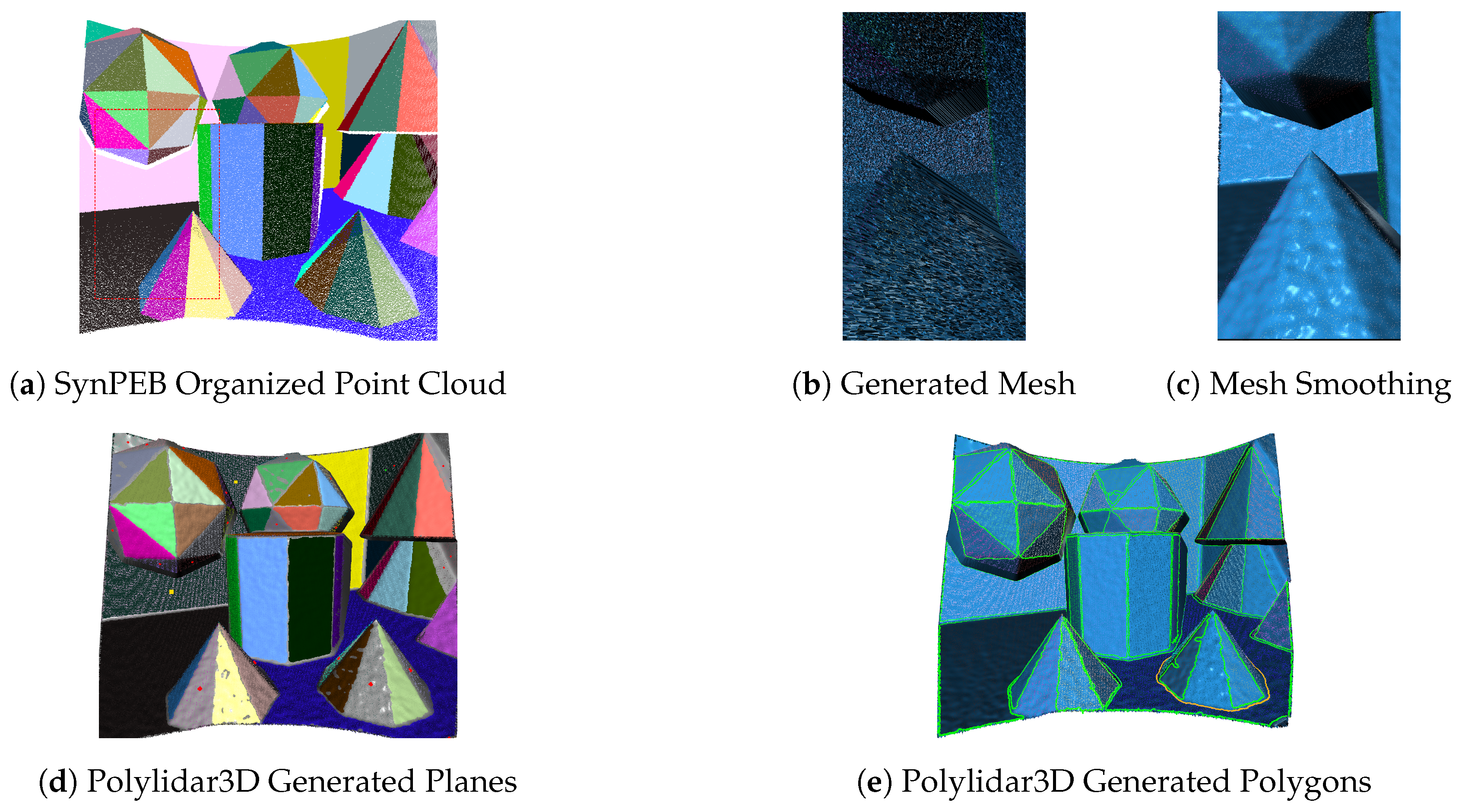
Figure 19.
Example SynPEB scene with the highest noise level. Point cloud, generated mesh, and mesh smoothed through Laplacian and bilateral filtering are shown in (a–c), respectively. Planes and polygons generated by Polylidar3D are shown in (d,e). Red, green, and yellow blocks in (d) represent missed, spurious, and oversegmented planes.
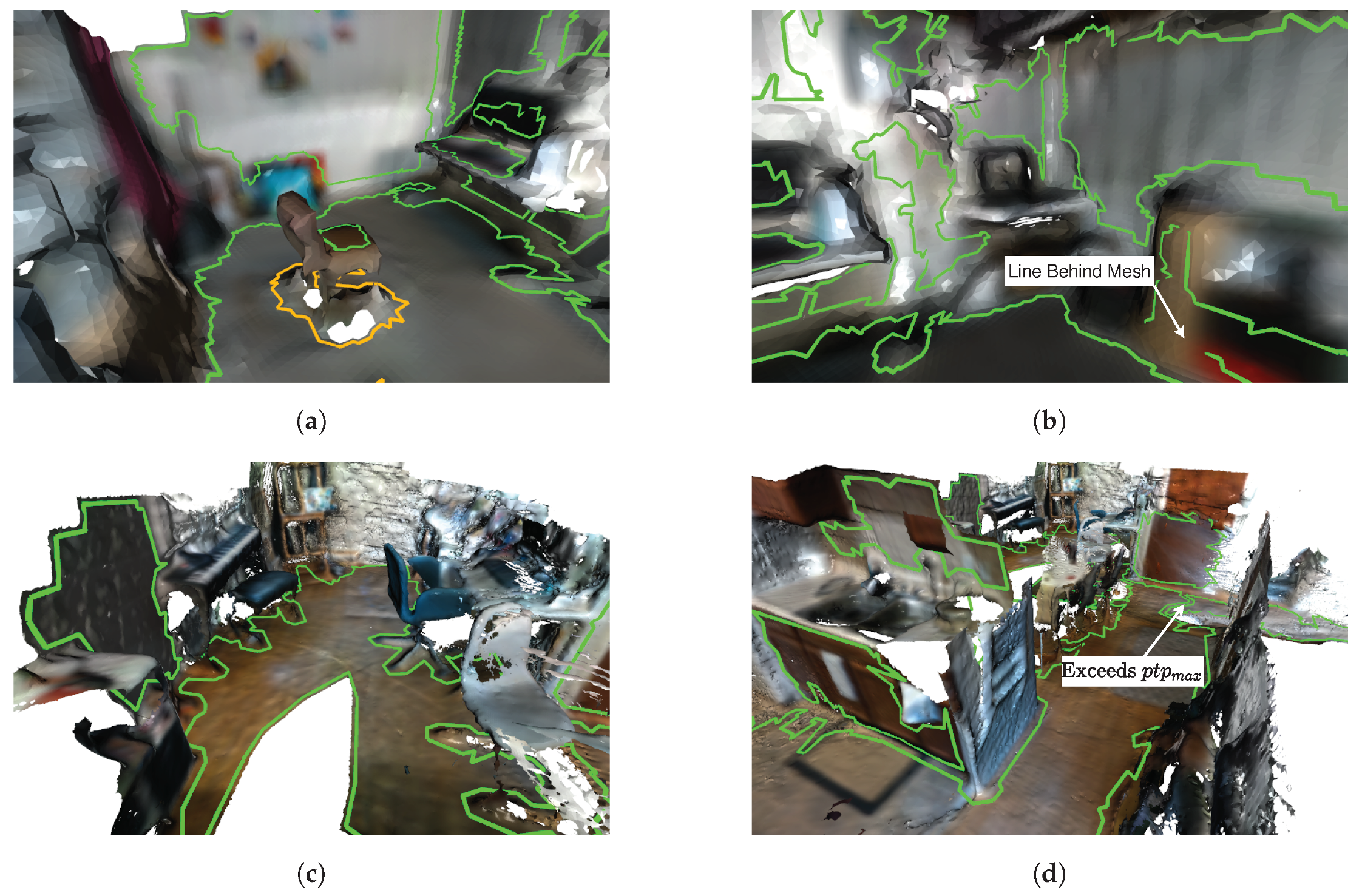
Figure 20.
Polygon extraction from meshes of an indoor home environment. (a,b) show results on a basement mesh which has a smoother approximation and less noise; (c,d) show results on a significantly larger, denser, and nosier mesh of the main floor.
Figure 20.
Polygon extraction from meshes of an indoor home environment. (a,b) show results on a basement mesh which has a smoother approximation and less noise; (c,d) show results on a significantly larger, denser, and nosier mesh of the main floor.
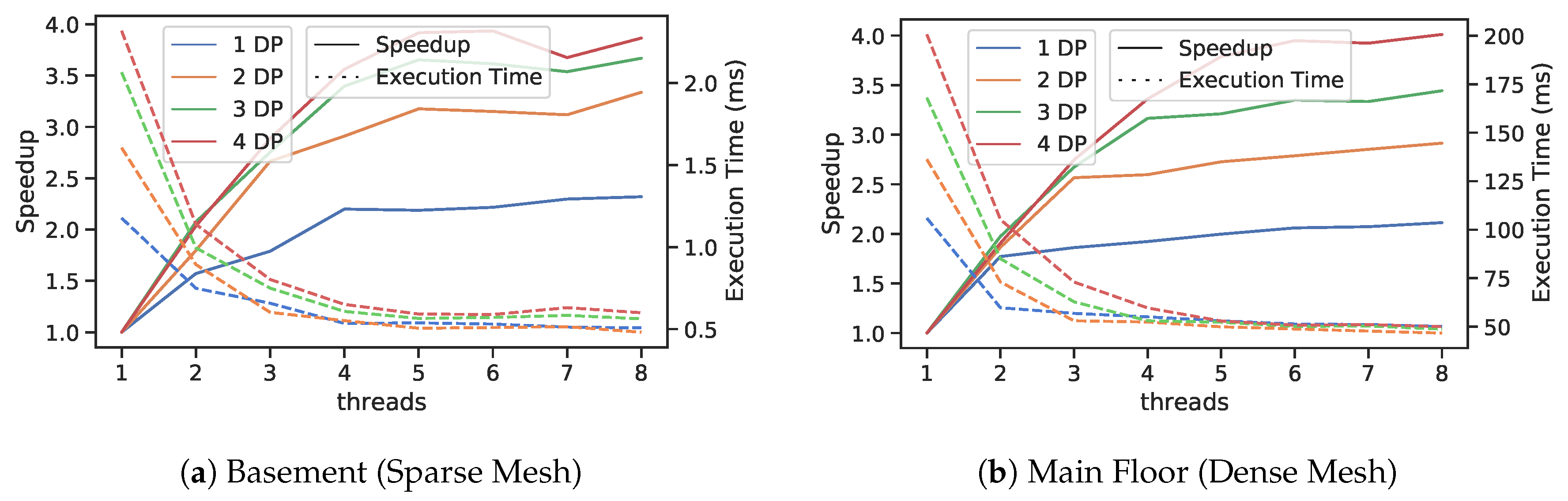
Figure 21.
Results of parallel speedup and execution timing of plane/polygon extraction with up to eight threads. Both basement (a) and main floor meshes (b) are analyzed. Solid lines indicate parallel speedup and link to the left y-axis while the dashed lines indicate execution time and link to the right y-axis. The color indicates number of dominant plane (DP) normals extracted.
Table 1.
Levels of Refinement for an Icosahedron.
Table 1.
Levels of Refinement for an Icosahedron.
| Level | # Vertices | # Triangles | Separation |
|---|
| 0 | 12 | 20 | |
| 1 | 42 | 80 | |
| 2 | 162 | 320 | |
| 3 | 642 | 1280 | |
| 4 | 2562 | 5120 | |
Table 2.
Execution Time Comparisons for Synthetic and Real World Datasets
Table 2.
Execution Time Comparisons for Synthetic and Real World Datasets
| Algorithm | Mean (ms) | Std (ms) |
|---|
| a Synthetic: 100,000 Random Normals |
| K-D tree | 20.0 | 0.1 |
| FastGA (ours) | 9.1 | 0.1 |
| b Real World: 60,620 Normals |
| K-D tree | 9.7 | 0.2 |
| FastGA (ours) | 4.4 | 0.1 |
Table 3.
Polylidar3D Parameters for Rooftop Detection.
Table 3.
Polylidar3D Parameters for Rooftop Detection.
| Algorithm | Parameters |
|---|
| Laplacian Filter | = 1.0, iterations = 2 |
| Bilateral Filter | = 0.1, = 0.1, iterations = 2 |
| Plane/Poly Extr. | = 200, = 0.94, = 0.9, = 8, |
| Poly. Filtering | , = 0.1, = 0.00, = 16, = 0.5 |
Table 4.
Polylidar3D Parameters for KITTI.
Table 4.
Polylidar3D Parameters for KITTI.
| Algorithm | Parameters |
|---|
| Plane/Poly Extr. | = 3500, = 0.97, = 1.25, = 6 |
| Poly. Filtering | , = 0.3, = 0.02, = 30, = 0.5 |
Table 5.
Mean Execution Timings (ms) of Polylidar3D on KITTI.
Table 5.
Mean Execution Timings (ms) of Polylidar3D on KITTI.
| Point Outlier Removal | Mesh Creation | Plane/Poly Ext. | Polygon Filtering | Total |
|---|
| 5.1 | 4.1 | 0.7 | 6.8 | 16.7 |
Table 6.
Intel RealSense SDK Post-processing Filter Parameters.
Table 6.
Intel RealSense SDK Post-processing Filter Parameters.
| Algorithm | Parameters |
|---|
| Decimation | magnitude = 2 |
| Temporal | = 0.3, = 60.0, persistence = 2 |
| Spatial | = 0.35, = 8.0, magnitude = 2, hole fill = 1 |
| Threshold | max distance = 2.5 m |
Table 7.
Polylidar3D Parameters for RealSense RGBD.
Table 7.
Polylidar3D Parameters for RealSense RGBD.
| Algorithm | Parameters |
|---|
| Laplacian Filter | = 1.0, kernel size = 3, iterations = 2 |
| Bilateral Filter | = 0.1, = 0.15, kernel size = 3, iterations = 2 |
| FastGA | level = 3, |
| Plane/Poly Extr. | = 500, = 0.96, = 0.05, , = 10 |
| Poly. Filtering | , = 0.02, = 0.005, = 0.1, = 0.1 |
Table 8.
Mean execution timings (ms) of Polylidar3D with RGBD data collected from indoor settings.
Table 8.
Mean execution timings (ms) of Polylidar3D with RGBD data collected from indoor settings.
| Scene | RS Filters | Mesh | Laplacian | Bilateral | FastGA | Plane/Poly Ext. | Poly. Filt. | Total |
|---|
| Basement | 2.4 | 0.4 | 0.4 | 0.5 | 1.2 | 1.7 | 4.8 | 11.4 |
| Main Floor | 2.4 | 0.4 | 0.4 | 0.5 | 1.3 | 1.6 | 5.1 | 11.7 |
Table 9.
Polylidar3D parameters for the SynPEB benchmark test set.
Table 9.
Polylidar3D parameters for the SynPEB benchmark test set.
| Algorithm | Parameters |
|---|
| Laplacian Filter | = 1.0, kernel size = 5, iterations = varies (predicted) |
| Bilateral Filter | = 0.1, = 0.1, kernel size = 3, iterations = 2 |
| FastGA | level = 5, |
| Plane/Poly Extr. | = 1000, = 0.95, = 0.1, , = 10 |
Table 10.
SynPEB Benchmark Results.
Table 10.
SynPEB Benchmark Results.
| Method | f [%] | k [%] | RMSE [mm] | | | | | time |
|---|
| PEAC [6] | 29.1 | 60.4 | 28.6 | 0.7 | 1.0 | 26.7 | 7.4 | 33 ms |
| MSAC [68] | 7.3 | 35.6 | 34.3 | 0.3 | 1.0 | 36.3 | 10.9 | 1.1 s |
| PPE [8] | 73.6 | 77.9 | 14.5 | 1.5 | 1.1 | 7.1 | 16.5 | 1.6 hr |
| Polylidar3D (proposed) | 47.3 | 78.3 | 7.2 | 0.1 | 0.3 | 22.8 | 4.9 | 34 ms |
Table 11.
Mean Execution Timings (ms) and Accuracy of Polylidar3D on SynPEB.
Table 11.
Mean Execution Timings (ms) and Accuracy of Polylidar3D on SynPEB.
| Point Cloud | Mesh Creation | Laplacian | Bilateral | FastGA | Plane/Poly Ext. | Total | f [%] |
|---|
| 500 × 500 | 9.3 | 1.1 | 3.0 | 6.6 | 14.9 | 33.9 | 47.3 |
| 250 × 250 | 2.0 | 0.5 | 0.7 | 2.5 | 4.1 | 9.8 | 44.6 |
Table 12.
Execution timing (ms) for one and five iterations of Laplacian filtering.
Table 12.
Execution timing (ms) for one and five iterations of Laplacian filtering.
| Data & Size | Ours | Open3D |
|---|
| CPU-S | CPU-M | GPU | CPU-S |
|---|
| SynPEB, 500 × 500 | 7.0; 35.0 | 2.0; 9.2 | 0.8; 0.9 | 205.9; 240.6 |
| RGBD, 120 × 212 | 0.7; 3.5 | 0.2; 0.9 | 0.1; 0.2 | 14.3; 17.5 |
Table 13.
Execution timing (ms) for one and five iterations of bilateral filtering.
Table 13.
Execution timing (ms) for one and five iterations of bilateral filtering.
| Data & Size | CPU-S | CPU-M | GPU |
|---|
| SynPEB, 500 × 500 | 73.0; 354.0 | 19.4; 90.9 | 3.2; 4.4 |
| RGBD, 120 × 212 | 7.2; 35.0 | 1.9; 9.2 | 0.5; 0.5 |
Table 14.
Polylidar3D Parameters for the Basement Mesh.
Table 14.
Polylidar3D Parameters for the Basement Mesh.
| Algorithm | Parameters |
|---|
| FastGA | level = 4, |
| Plane/Poly Extr. | = 80, = 0.95, = 0.1, , = 6 |
| Poly. Filtering | , = 0.025, = 0.0, = 0.07, = 0.05 |
Table 15.
Polylidar3D Parameters for the Main Floor Mesh.
Table 15.
Polylidar3D Parameters for the Main Floor Mesh.
| Algorithm | Parameters |
|---|
| FastGA | level = 4, |
| Plane/Poly Extr. | = 1000, = 0.95, = 0.1, , = 6 |
| Poly. Filtering | , = 0.05, = 0.02, = 0.25, = 0.1 |


