Dynamic Camera Reconfiguration with Reinforcement Learning and Stochastic Methods for Crowd Surveillance †

 ,
,  ,
,
Abstract
1. Introduction
2. Related Work
3. Method
3.1. Observation Model
- an observation vector , which represents the number of pedestrians detected for each cell ;
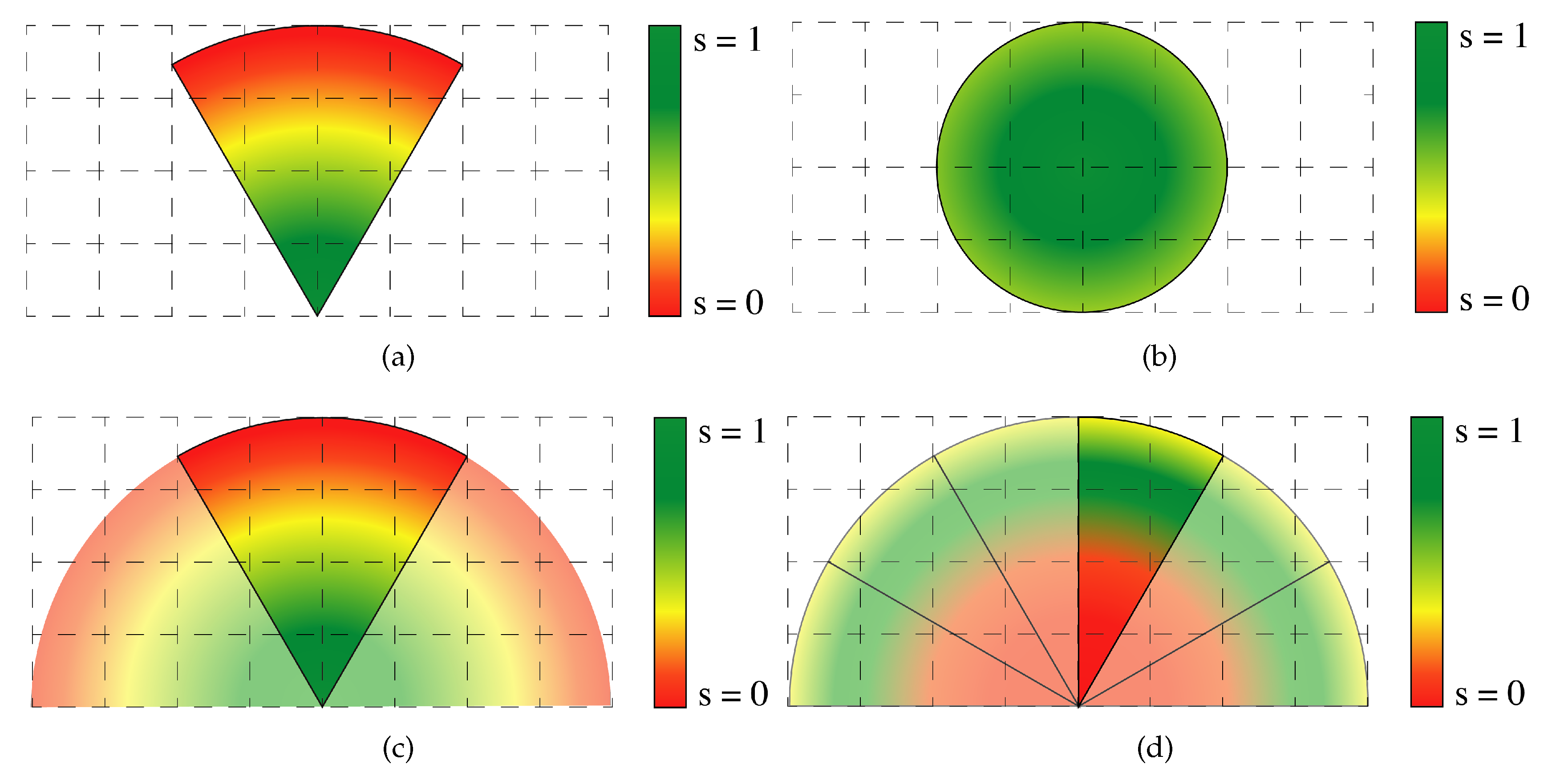
- a spatial confidence vector , which describes the confidence of the measures for each cell . Our spatial confidence depends only on the relative geometric position of the observing camera and the observed cell;
- a temporal confidence vector , which depends on the time passed since the cell has last been observed; and
- an overall confidence vector , which depends on the temporal and spatial confidences.
3.2. Camera Models
3.2.1. Fixed Cameras
3.2.2. PTZ Cameras
3.2.3. UAV-Based Cameras
3.3. Reconfiguration Objective
3.4. Reconfiguration Objectives: Custom Policies
- The reconfiguration objectives are the same for the different camera types, namely UAVs and PTZs. In the real world, UAVs have a higher cost of deployment and movement with respect to PTZs, while they provide more degrees of freedom for their reconfigurability.
- The priority maps do not share information about camera type and position between different cameras. Especially in the case of UAVs, this can lead to a superposition of different cameras, which decrease the network performances.
3.5. Update Function
3.6. Local Camera Decision: Greedy Approach
3.7. Evaluation Metrics
3.8. Reinforcement Learning
- a set of states , which encode the local visual observation of each UAV,
- a set of possible actions that each UAV can choose to perform at the next time step and
- a set of rewards , which depend on the observation vector and its related confidence .
4. Experimental Results
- s
- m
- fixed and PTZ cameras height m
- UAV-based cameras height m
4.1. Quantitative Results
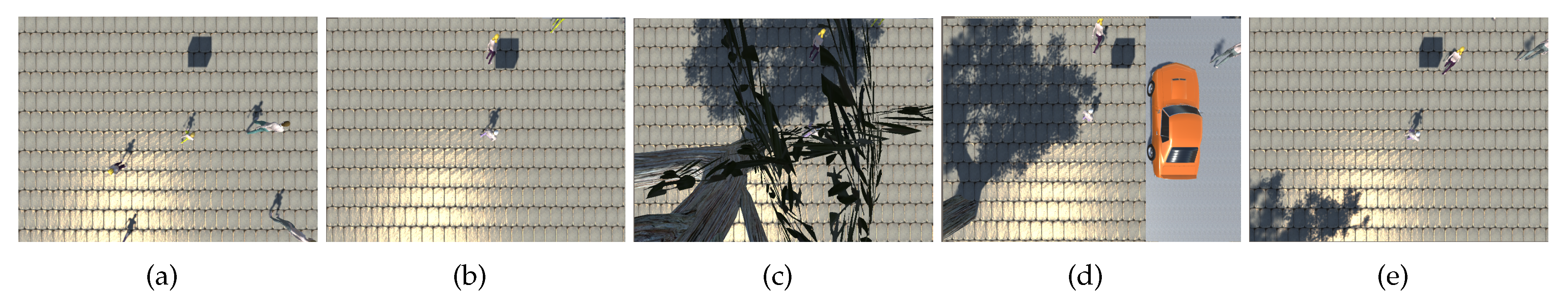
4.2. Qualitative Results
5. Conclusions
Author Contributions
Funding
Conflicts of Interest
References
- Konda, K.R.; Conci, N. Optimal configuration of PTZ camera networks based on visual quality assessment and coverage maximization. In Proceedings of the 2013 Seventh International Conference on Distributed Smart Cameras (ICDSC), Palm Springs, CA, USA, 29 October–1 November 2013; pp. 1–8. [Google Scholar]
- Lewis, P.; Esterle, L.; Chandra, A.; Rinner, B.; Yao, X. Learning to be different: Heterogeneity and efficiency in distributed smart camera networks. In Proceedings of the 2013 IEEE 7th International Conference on Self-Adaptive and Self-Organizing Systems, Philadelphia, PA, USA, 9–13 September 2013; pp. 209–218. [Google Scholar]
- Reisslein, M.; Rinner, B.; Roy-Chowdhury, A. Smart Camera Networks. IEEE Comput. 2014, 47, 23–25. [Google Scholar]
- Yao, Z.; Zhang, G.; Lu, D.; Liu, H. Data-driven crowd evacuation: A reinforcement learning method. Neurocomputing 2019, 366, 314–327. [Google Scholar] [CrossRef]
- Qureshi, F.Z.; Terzopoulos, D. Surveillance in virtual reality: System design and multi-camera control. In Proceedings of the 2007 IEEE Conference on Computer Vision and Pattern Recognition, Minneapolis, MN, USA, 17–22 June 2007; pp. 1–8. [Google Scholar]
- Taylor, G.R.; Chosak, A.J.; Brewer, P.C. Ovvv: Using virtual worlds to design and evaluate surveillance systems. In Proceedings of the 2007 IEEE Conference on Computer Vision and Pattern Recognition, Minneapolis, MN, USA, 17–22 June 2007; pp. 1–8. [Google Scholar]
- Altahir, A.A.; Asirvadam, V.S.; Hamid, N.H.B.; Sebastian, P.; Hassan, M.A.; Saad, N.B.; Ibrahim, R.; Dass, S.C. Visual Sensor Placement Based on Risk Maps. IEEE Trans. Instrum. Meas. 2019, 69, 3109–3117. [Google Scholar] [CrossRef]
- Bour, P.; Cribelier, E.; Argyriou, V. Crowd behavior analysis from fixed and moving cameras. In Multimodal Behavior Analysis in the Wild; Academic Press: Cambridge, MA, USA, 2019; pp. 289–322. [Google Scholar]
- Bisagno, N.; Conci, N.; Rinner, B. Dynamic Camera Network Reconfiguration for Crowd Surveillance. In Proceedings of the 12th International Conference on Distributed Smart Cameras, Eindhoven, The Netherlands, 3–4 September 2018; pp. 1–6. [Google Scholar]
- Motlagh, N.H.; Bagaa, M.; Taleb, T. UAV-based IoT platform: A crowd surveillance use case. IEEE Commun. Mag. 2017, 55, 128–134. [Google Scholar] [CrossRef]
- Shakhatreh, H.; Sawalmeh, A.H.; Al-Fuqaha, A.; Dou, Z.; Almaita, E.; Khalil, I.; Othman, N.S.; Khreishah, A.; Guizani, M. Unmanned aerial vehicles (UAVs): A survey on civil applications and key research challenges. IEEE Access 2019, 7, 48572–48634. [Google Scholar] [CrossRef]
- Hatanaka, T.; Wasa, Y.; Funada, R.; Charalambides, A.G.; Fujita, M. A payoff-based learning approach to cooperative environmental monitoring for PTZ visual sensor networks. IEEE Trans. Autom. Control 2015, 61, 709–724. [Google Scholar] [CrossRef]
- Khan, M.I.; Rinner, B. Resource coordination in wireless sensor networks by cooperative reinforcement learning. In Proceedings of the 2012 IEEE International Conference on Pervasive Computing and Communications Workshops, Lugano, Switzerland, 19–23 March 2012; pp. 895–900. [Google Scholar]
- Khan, U.A.; Rinner, B. A reinforcement learning framework for dynamic power management of a portable, multi-camera traffic monitoring system. In Proceedings of the 2012 IEEE International Conference on Green Computing and Communications, Besancon, France, 20–23 November 2012; pp. 557–564. [Google Scholar]
- Rudolph, S.; Edenhofer, S.; Tomforde, S.; Hähner, J. Reinforcement learning for coverage optimization through PTZ camera alignment in highly dynamic environments. In Proceedings of the International Conference on Distributed Smart Cameras, Venezia Mestre, Italy, 4–7 November 2014; pp. 1–6. [Google Scholar]
- Helbing, D.; Molnar, P. Social force model for pedestrian dynamics. Phys. Rev. E 1995, 51, 4282. [Google Scholar] [CrossRef] [PubMed]
- Micheloni, C.; Rinner, B.; Foresti, G.L. Video Analysis in PTZ Camera Networks - From master-slave to cooperative smart cameras. IEEE Signal Process Mag. 2010, 27, 78–90. [Google Scholar] [CrossRef]
- Foresti, G.L.; Mähönen, P.; Regazzoni, C.S. Multimedia Video-Based Surveillance Systems: Requirements, Issues and Solutions; Springer Science & Business Media: Philadelphia, NY, USA, 2000; Volume 573. [Google Scholar]
- Shah, M.; Javed, O.; Shafique, K. Automated visual surveillance in realistic scenarios. IEEE MultiMedia 2007, 14, 30–39. [Google Scholar] [CrossRef]
- Junior, J.C.S.J.; Musse, S.R.; Jung, C.R. Crowd analysis using computer vision techniques. IEEE Signal Process Mag. 2010, 27, 66–77. [Google Scholar]
- Azzari, P.; Di Stefano, L.; Bevilacqua, A. An effective real-time mosaicing algorithm apt to detect motion through background subtraction using a PTZ camera. In Proceedings of the IEEE Conference on Advanced Video and Signal Based Surveillance, Como, Italy, 15–16 September 2005; pp. 511–516. [Google Scholar]
- Kang, S.; Paik, J.K.; Koschan, A.; Abidi, B.R.; Abidi, M.A. Real-time video tracking using PTZ cameras. Sixth International Conference on Quality Control by Artificial Vision. Proc. SPIE Int. Soc. Opt. Eng. 2003, 103–112. [Google Scholar] [CrossRef]
- Bevilacqua, A.; Azzari, P. High-quality real time motion detection using ptz cameras. In Proceedings of the IEEE International Conference on Advanced Video and Signal Based Surveillance, Sydney, Australia, 22–24 November 2006; p. 23. [Google Scholar]
- Rinner, B.; Esterle, L.; Simonjan, J.; Nebehay, G.; Pflugfelder, R.; Dominguez, G.F.; Lewis, P.R. Self-aware and self-expressive camera networks. IEEE Computer 2014, 48, 21–28. [Google Scholar] [CrossRef]
- Ryan, A.; Zennaro, M.; Howell, A.; Sengupta, R.; Hedrick, J.K. An overview of emerging results in cooperative UAV control. In Proceedings of the 43rd IEEE Conference on Decision and Control, Nassau, Bahamas, 14–17 December 2004; pp. 602–607. [Google Scholar]
- Yanmaz, E.; Yahyanejad, S.; Rinner, B.; Hellwagner, H.; Bettstetter, C. Drone networks: Communications, coordination, and sensing. Ad Hoc Networks 2018, 68, 1–15. [Google Scholar] [CrossRef]
- Khan, A.; Rinner, B.; Cavallaro, A. Cooperative Robots to Observe Moving Targets: A Review. IEEE Trans. Cybern. 2018, 48, 187–198. [Google Scholar] [CrossRef] [PubMed]
- Yao, H.; Cavallaro, A.; Bouwmans, T.; Zhang, Z. Guest Editorial Introduction to the Special Issue on Group and Crowd Behavior Analysis for Intelligent Multicamera Video Surveillance. IEEE Trans. Circuits Syst. Video Technol. 2017, 27, 405–408. [Google Scholar] [CrossRef]
- Sutton, R.S.; Barto, A.G. Reinforcement learning: An introduction; MIT Press: Cambridge, London, UK, 2018. [Google Scholar]
- Esterle, L. Centralised, decentralised, and self-organised coverage maximisation in smart camera networks. In Proceedings of the 2017 IEEE 11th International Conference on Self-Adaptive and Self-Organizing Systems (SASO), Tucson, AZ, USA, 18–22 September 2017; pp. 1–10. [Google Scholar]
- Vejdanparast, A.; Lewis, P.R.; Esterle, L. Online zoom selection approaches for coverage redundancy in visual sensor networks. In Proceedings of the 12th International Conference on Distributed Smart Cameras, Eindhoven, The Netherlands, 3–4 September 2018; pp. 1–6. [Google Scholar]
- Jones, M.; Viola, P. Fast Multi-View Face Detection; Technical Report TR-20003-96; Mitsubishi Electric Research Lab.: Cambridge, MA, USA, 2003; Volume 3. [Google Scholar]
- Juliani, A.; Berges, V.P.; Teng, E.; Cohen, A.; Harper, J.; Elion, C.; Goy, C.; Gao, Y.; Henry, H.; Mattar, M.; et al. Unity: A General Platform for Intelligent Agents. arXiv 2018, arXiv:cs.LG/1809.02627. [Google Scholar]
- Haarnoja, T.; Zhou, A.; Abbeel, P.; Levine, S. Soft Actor-Critic: Off-Policy Maximum Entropy Deep Reinforcement Learning with a Stochastic Actor. arXiv 2018, arXiv:cs.LG/1801.01290. [Google Scholar]


| ID | g and p | GCM | PCM | |
|---|---|---|---|---|
| 1 | 0.2 | 0 | 12.4% | 17.4% |
| 2 | 0.2 | 0.5 | 14.3% | 20.5% |
| 3 | 0.2 | 1 | 10.4% | 13.5% |
| 4 | 0.01 | 0 | 42.9% | 47.6% |
| 5 | 0.01 | 0.5 | 30.3% | 33.1% |
| 6 | 0.01 | 1 | 22.9% | 28.2% |
| 7 | 0.01 | 0 | 43.1% | 45.6% |
| 8 | 0.01 | 0.5 | 28.7% | 54.4% |
| 9 | 0.01 | 1 | 26.1% | 61.2% |
| Split Priority | Position Aware | ||||||
|---|---|---|---|---|---|---|---|
| ID | g and p | ffPTZ | ffUAV | GCM | PCM | GCM | PCM |
| 10 | 0.2 | 0 | 0 | 15.6% | 18.8% | 15.5% | 20.3% |
| 11 | 0.2 | 0.5 | 0 | 16.7% | 18.8% | 16.7% | 19.1% |
| 12 | 0.2 | 1 | 0 | 16.8% | 18.5% | 16.6% | 20.6% |
| 13 | 0.2 | 0 | 0.5 | 11.3% | 14.4% | 15.5% | 20.7% |
| 14 | 0.2 | 0.5 | 0.5 | 11.5% | 14.3% | 16.7% | 21.8% |
| 15 | 0.2 | 1 | 0.5 | 11.5% | 12.0% | 16.5% | 21.2% |
| 16 | 0.2 | 0 | 1 | 11.3% | 11.6% | 15.5% | 20.4% |
| 17 | 0.2 | 0.5 | 1 | 11.5% | 14.0% | 16.3% | 19.1% |
| 18 | 0.2 | 1 | 1 | 11.5% | 11.2% | 16.1% | 20.4% |
| ID | g and p | GCM | PCM | |
|---|---|---|---|---|
| 19 | 0.2 | 0 | ||
| 20 | 0.2 | 0.5 | ||
| 21 | 0.2 | 1 | ||
| 22 | 0.01 | 0 | ||
| 23 | 0.01 | 0.5 | ||
| 24 | 0.01 | 1 |
© 2020 by the authors. Licensee MDPI, Basel, Switzerland. This article is an open access article distributed under the terms and conditions of the Creative Commons Attribution (CC BY) license (http://creativecommons.org/licenses/by/4.0/).
Share and Cite
Bisagno, N.; Xamin, A.; De Natale, F.; Conci, N.; Rinner, B. Dynamic Camera Reconfiguration with Reinforcement Learning and Stochastic Methods for Crowd Surveillance. Sensors 2020, 20, 4691. https://doi.org/10.3390/s20174691
Bisagno N, Xamin A, De Natale F, Conci N, Rinner B. Dynamic Camera Reconfiguration with Reinforcement Learning and Stochastic Methods for Crowd Surveillance. Sensors. 2020; 20(17):4691. https://doi.org/10.3390/s20174691
Chicago/Turabian StyleBisagno, Niccolò, Alberto Xamin, Francesco De Natale, Nicola Conci, and Bernhard Rinner. 2020. "Dynamic Camera Reconfiguration with Reinforcement Learning and Stochastic Methods for Crowd Surveillance" Sensors 20, no. 17: 4691. https://doi.org/10.3390/s20174691
APA StyleBisagno, N., Xamin, A., De Natale, F., Conci, N., & Rinner, B. (2020). Dynamic Camera Reconfiguration with Reinforcement Learning and Stochastic Methods for Crowd Surveillance. Sensors, 20(17), 4691. https://doi.org/10.3390/s20174691