Nonlinear Chemical Process Fault Diagnosis Using Ensemble Deep Support Vector Data Description


Abstract
1. Introduction
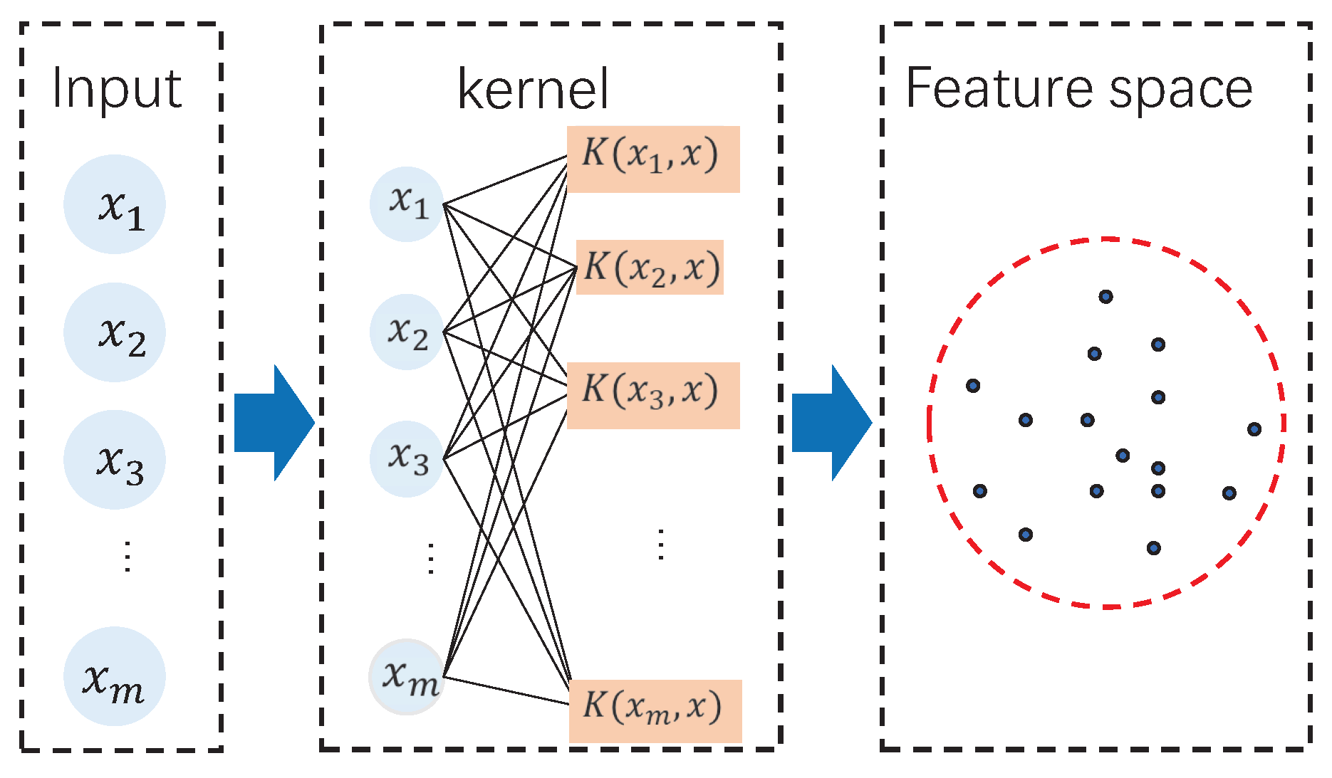
2. SVDD Method
3. Fault Diagnosis Method Based on Ensemble Deep SVDD
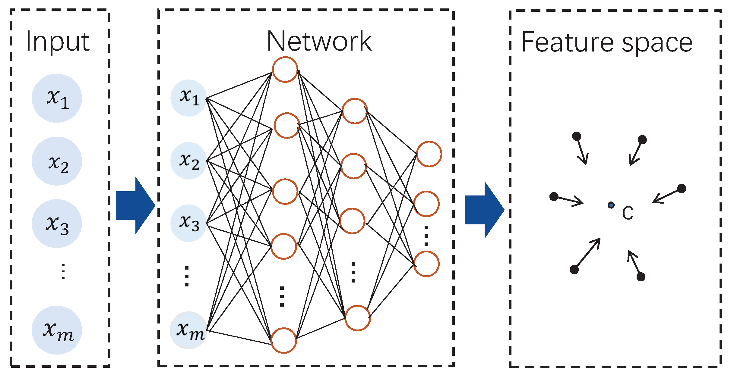
3.1. Deep SVDD Model Construction
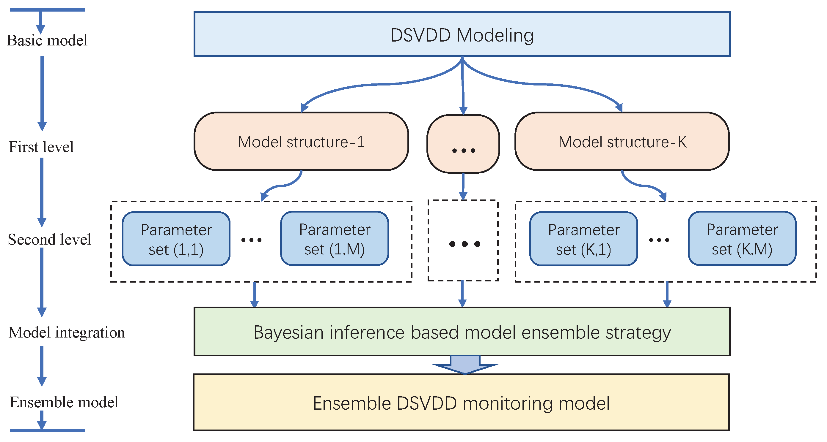
3.2. Multiple Deep Models Ensemble with Bayesian Inference Strategy
3.3. Fault Variable Isolation Using Distance Correlation
3.4. Process Monitoring Procedure
- Offline modeling stage:
- Collect the historical normal data and divide them into the training data set and validating data set;
- Normalize all the data sets by the mean and variance of the training data set;
- Apply the normal data set to pretrain the deep SVDD networks with autoencoder to determine the center vector;
- Train the multiple deep SVDD networks as the basic monitoring sub-models.
- Compute the monitoring indices of the validation data and determine the confidence limits using KDE method;
- Construct the ensemble statistic by Bayesian fusion strategy, and calculate its detection threshold .
- Online monitoring stage:
- Collect testing sample and normalize it with the mean and variance of the training data set;
- Project the normalized data onto each deep SVDD model and obtain its monitoring indices ;
- Compute the ensemble index and compare it with the threshold . If , that means one fault occurs. Otherwise, the process is in the normal status.
- When a fault is detected, the fault isolation map is built to identify the fault cause variables.
4. Case Study
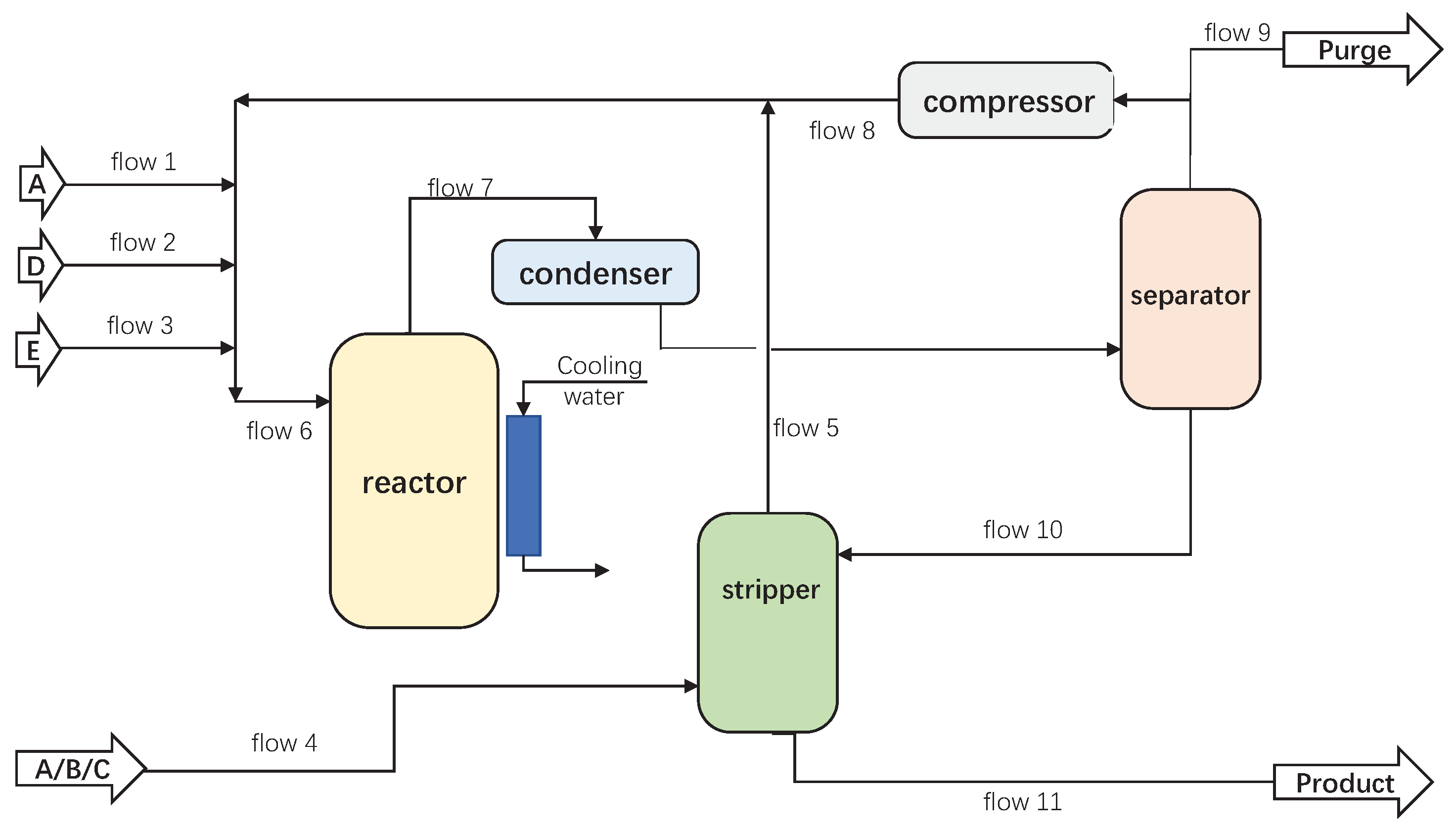
4.1. Process Description
4.2. Results and Discussions
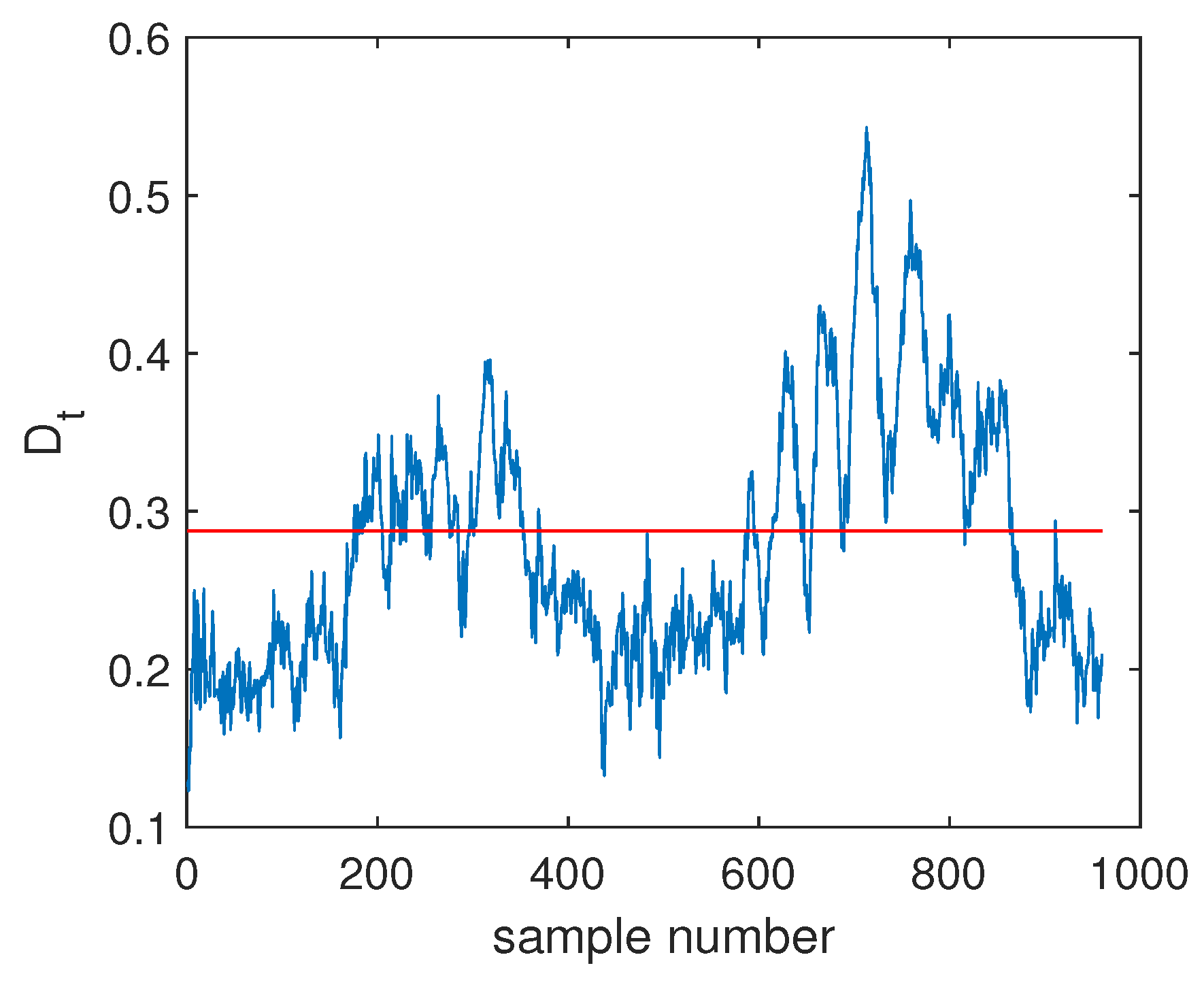
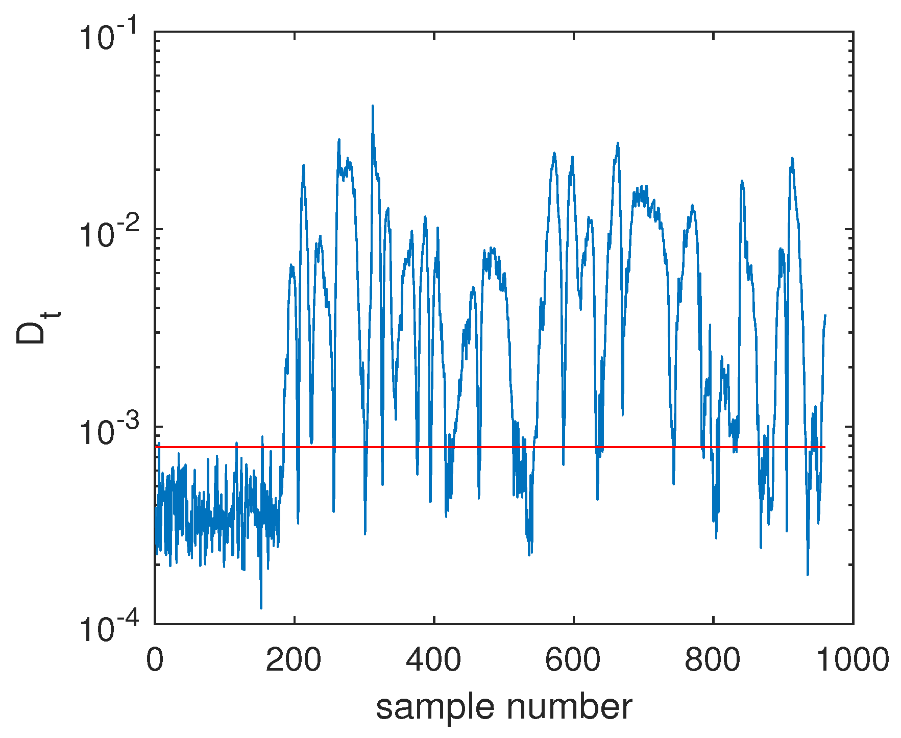
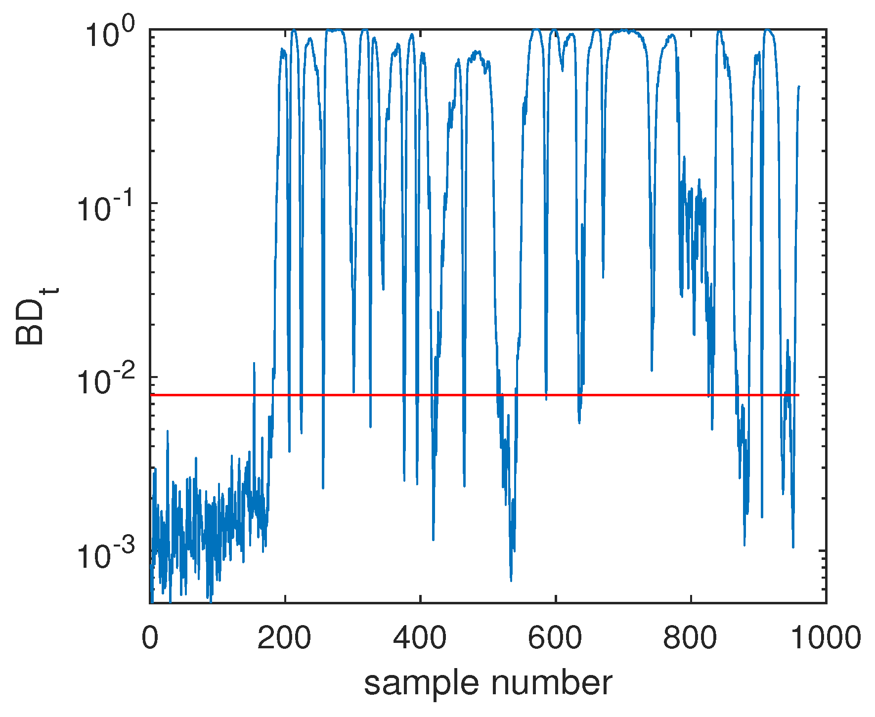
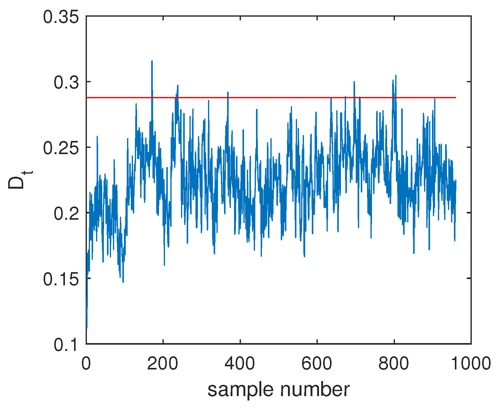
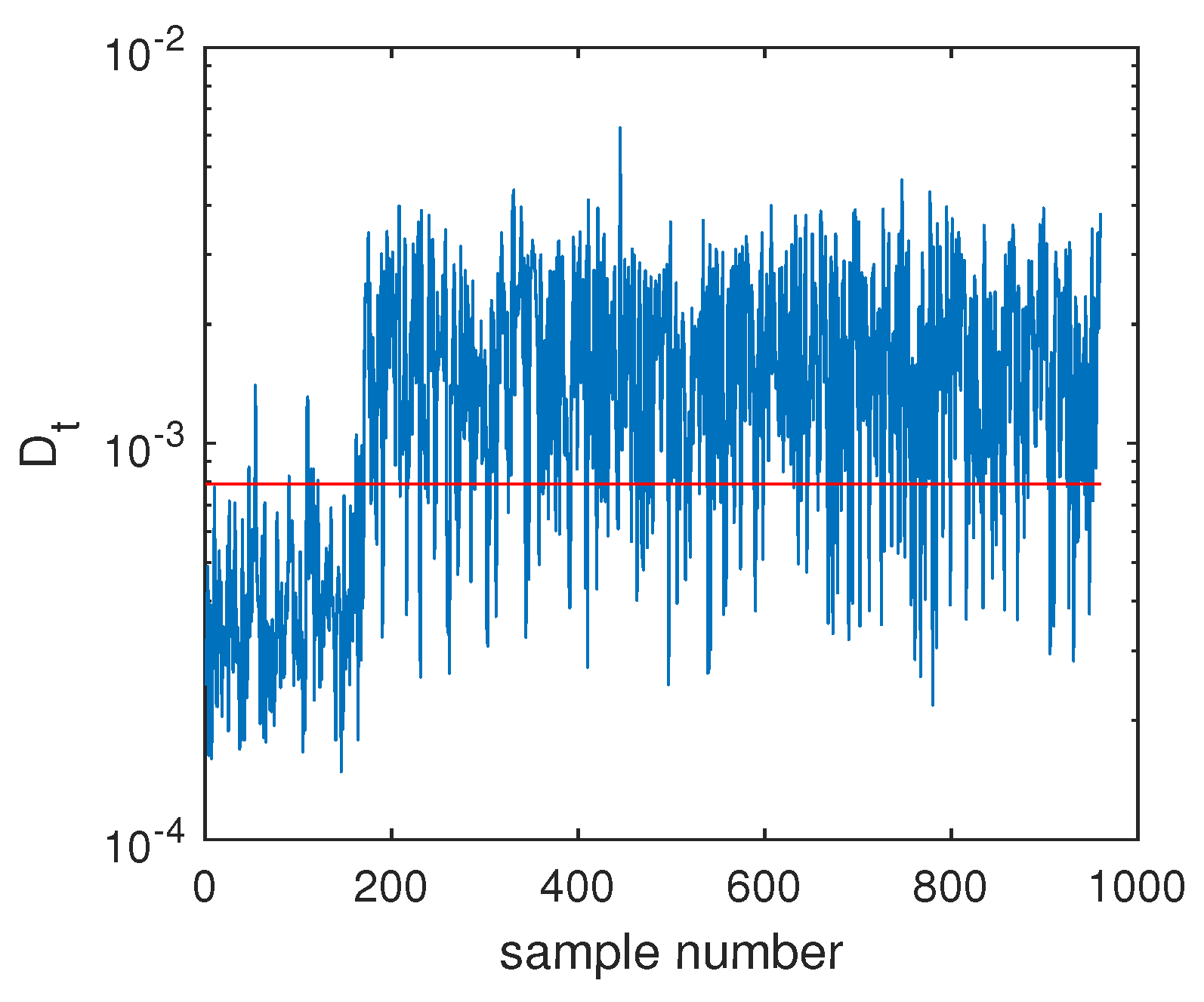
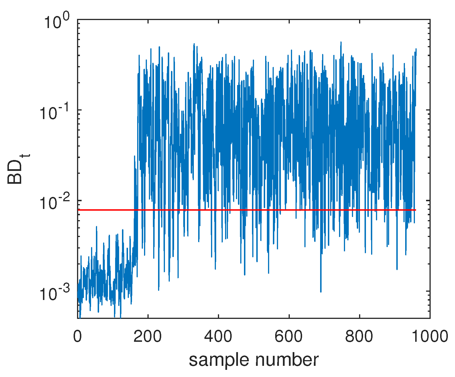
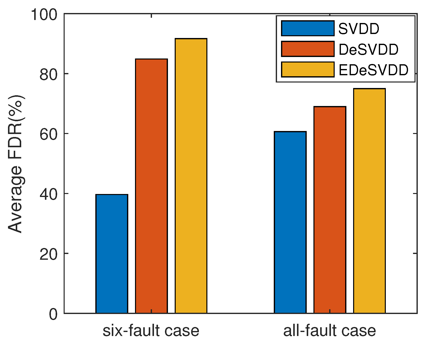
4.2.1. Fault Detection
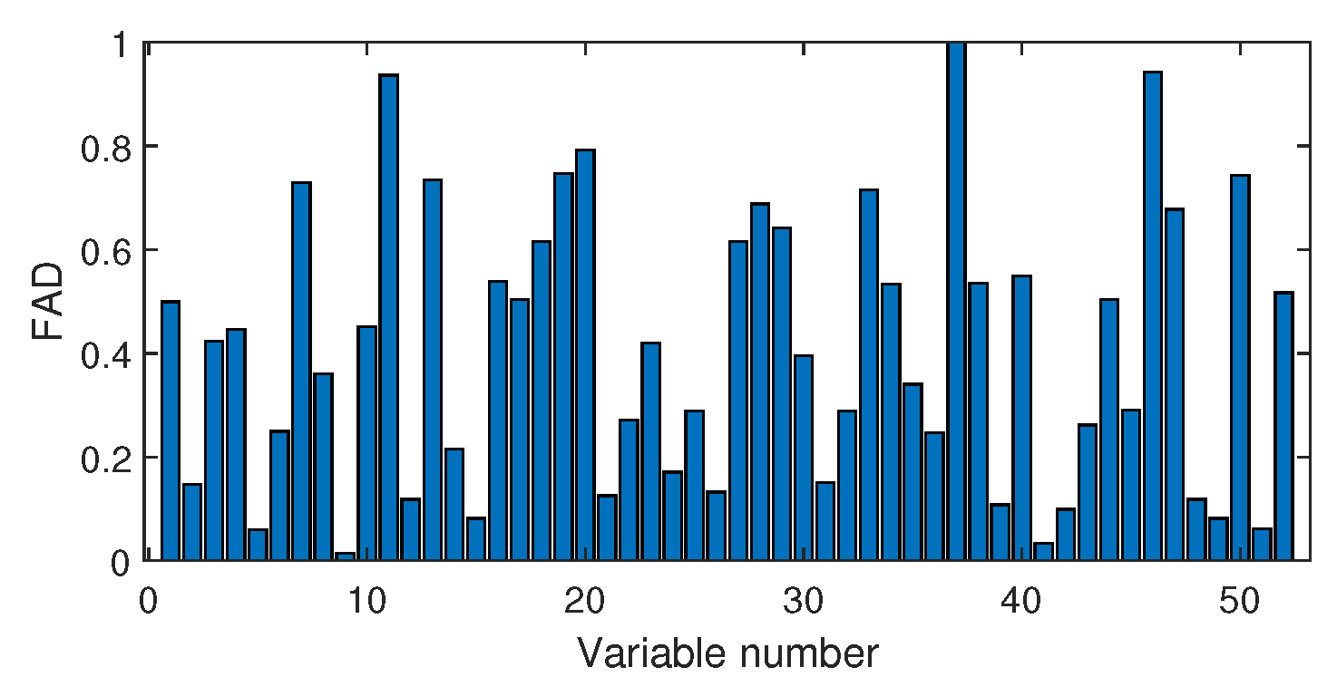
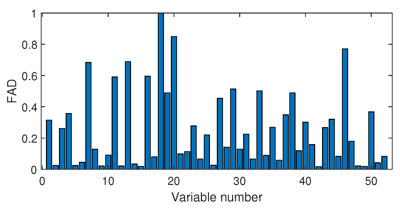
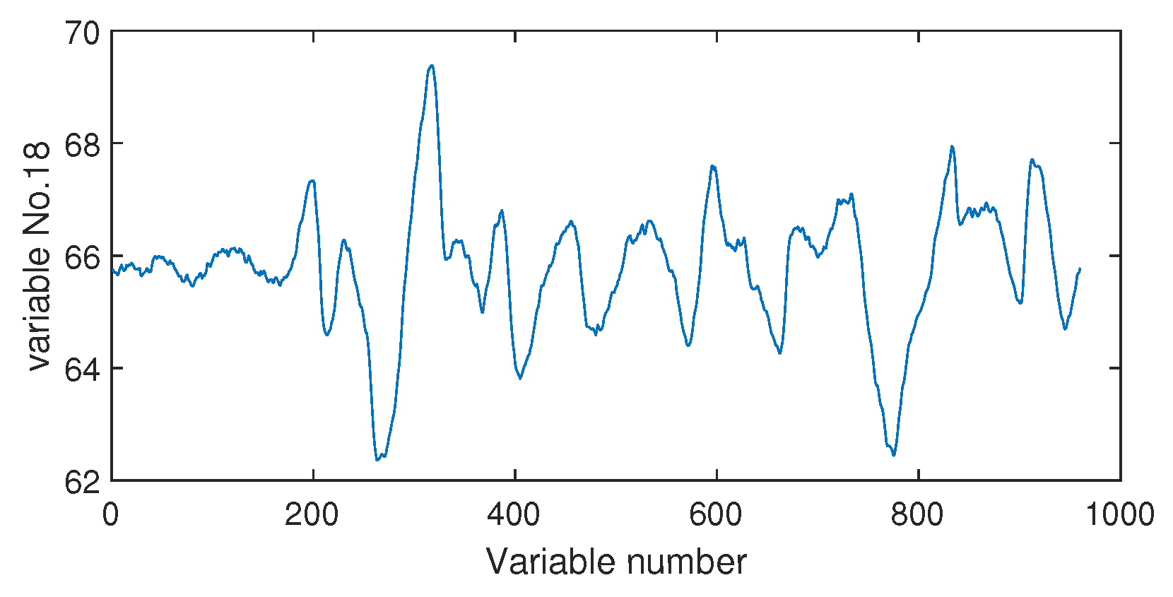
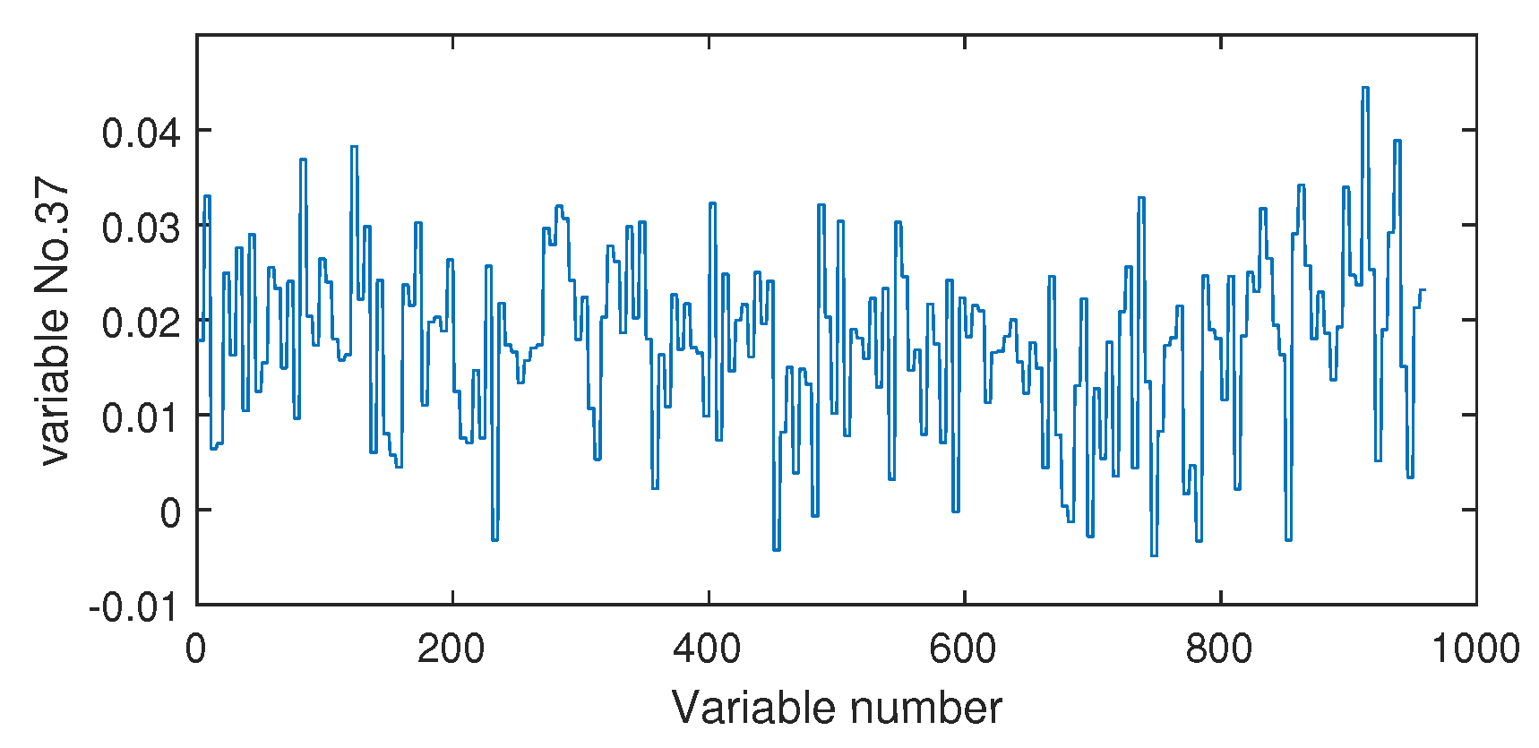
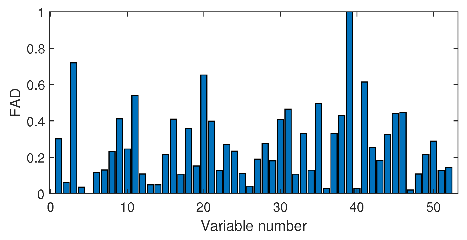
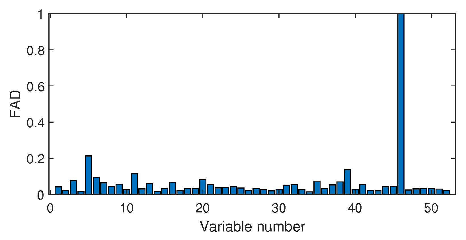
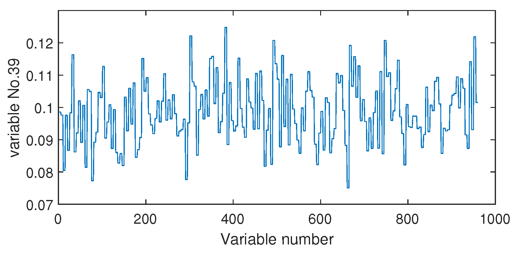
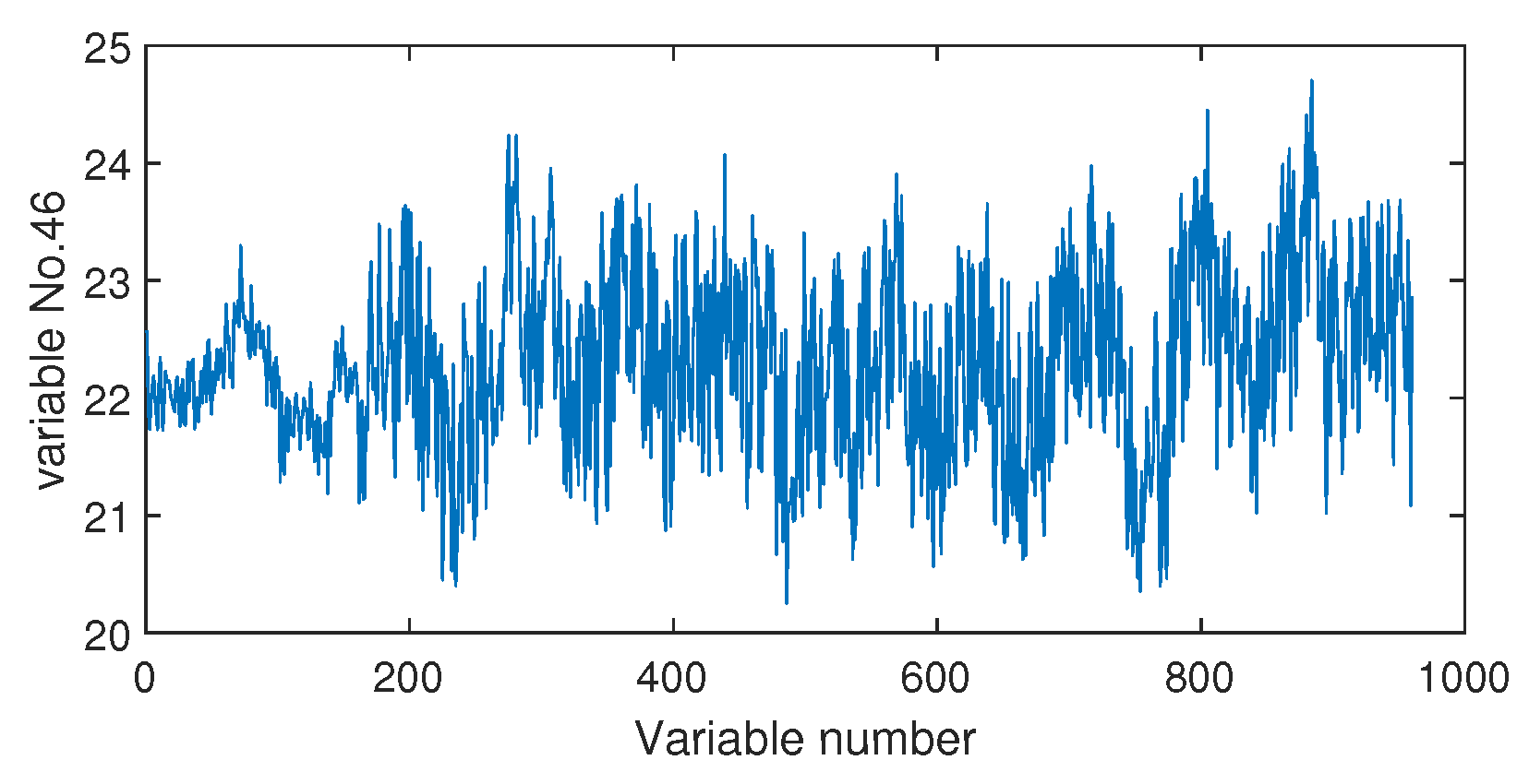
4.2.2. Fault Isolation
5. Conclusions
Author Contributions
Funding
Conflicts of Interest
References
- Chen, Z.; Cao, Y.; Ding, S.X.; Zhang, K.; Koenings, T.; Peng, T.; Yang, C.; Gui, W. A distributed canonical correlation analysis-Based fault detection method for plant-wide process monitoring. IEEE Trans. Ind. Inform. 2019, 15, 2710–2720. [Google Scholar] [CrossRef]
- Deng, X.; Cai, P.; Cao, Y.; Wang, P. Two-step localized kernel principal component analysis based incipient fault diagnosis for nonlinear industrial processes. Ind. Eng. Chem. Res. 2020, 59, 5956–5968. [Google Scholar] [CrossRef]
- Cui, P.; Zhang, C.; Yang, Y. Improved nonlinear process monitoring based on ensemble KPCA with local structure analysis. Chem. Eng. Res. Des. 2019, 142, 355–368. [Google Scholar] [CrossRef]
- Li, G.; Hu, Y.; Chen, H.; Li, H. A sensor fault detection and diagnosis strategy for screw chiller system using support vector data description-based D-statistic and DV-contribution. Energy Build. 2016, 133, 230–245. [Google Scholar] [CrossRef]
- Zhang, C.; Peng, K.; Dong, J. An incipient fault detection and self-learning identification method based on robust SVDD and RBM-PNN. J. Process Contr. 2020, 85, 173–183. [Google Scholar] [CrossRef]
- Tax, D.M.J.; Duin, R.P.W. Support vector domain description. Pattern Recogn. Lett. 1999, 20, 1191–1199. [Google Scholar] [CrossRef]
- Tax, D.M.J.; Duin, R.P.W. Support vector data description. Mach. Learn. 2004, 54, 45–66. [Google Scholar] [CrossRef]
- GhasemiGol, M.; Monsefi, R.; Sadoghi-Yazdi, H. Intrusion detection by ellipsoid boundary. J. Netw. Syst. Manag. 2010, 18, 265–282. [Google Scholar] [CrossRef]
- Sindagi, V.A.; Srivastava, S. Domain adaptation for automatic OLED panel defect detection using adaptive support vector data description. Int. J. Comput. Vis. 2017, 122, 193–211. [Google Scholar] [CrossRef]
- Chen, Y.; Li, S. A lightweight anomaly detection method based on SVDD for wireless networks. Wirel. Pers. Commun. 2019, 105, 1235–1256. [Google Scholar] [CrossRef]
- Ge, Z.; Gao, F.; Song, Z. Batch process monitoring based on support vector data description method. J. Process Contr. 2011, 21, 949–959. [Google Scholar] [CrossRef]
- Jiang, Q.; Yan, X. Probabilistic weighted npe-svdd for chemical process monitoring. Control Eng. Pract. 2014, 28, 74–89. [Google Scholar] [CrossRef]
- Huang, J.; Yan, X. Related and independent variable fault detection based on KPCA and SVDD. J. Process Contr. 2016, 28, 88–99. [Google Scholar] [CrossRef]
- Li, H.; Wang, H.; Fan, W. Multimode process fault detection based on local density ratio-weighted support vector data description. Ind. Eng. Chem. Res. 2017, 56, 2475–2491. [Google Scholar] [CrossRef]
- Lv, Z.; Yan, X.; Jiang, Q.; Li, N. Just-in-time learning-multiple subspace support vector data description used for non-Gaussian dynamic batch process monitoring. J. Chemometr. 2019, 33, 1–13. [Google Scholar] [CrossRef]
- Dong, Q.; Kontar, R.; Li, M.; Xu, G. A simple approach to multivariate monitoring of production processes with non-Gaussian data. J. Manuf. Syst. 2019, 53, 291–304. [Google Scholar] [CrossRef]
- Liu, C.; Gryllias, K. A semi-supervised support vector data description-based fault detection method for rolling element bearings based on cyclic spectral analysis. Mech. Syst. Signal Proc. 2020, 140, 1–24. [Google Scholar] [CrossRef]
- Zhang, H.; Tian, X.; Wang, X.; Gao, Y. Local and global unsupervised kernel extreme learning machine and its application in nonlinear process fault detection. In Proceedings of the International Conference on Extreme Learning Machine (ELM), Hangzhou, China, 15–17 December 2015. [Google Scholar]
- Lv, Z.; Yan, X.; Jiang, Q. Batch process monitoring based on self-adaptive subspace support vector data description. Chemom. Intell. Lab. Syst. 2017, 170, 25–31. [Google Scholar] [CrossRef]
- Zgarni, S.; Keskes, H.; Braham, A. Nested SVDD in DAG SVM for induction motor condition monitoring. Eng. Appl. Artif. Intell. 2018, 71, 210–215. [Google Scholar] [CrossRef]
- LeCun, Y.; Bengio, Y.; Hinton, G. Deep learning. Nature 2015, 521, 436–444. [Google Scholar] [CrossRef]
- Schmidhuber, J. Deep learning in neural networks. Neural Netw. 2015, 61, 85–117. [Google Scholar] [CrossRef] [PubMed]
- Wu, Y.; Lin, M.; Rohani, S. Particle characterization with on-line imaging and neural network image analysis. Chem. Eng. Res. Des. 2020, 157, 114–125. [Google Scholar] [CrossRef]
- Ruff, L.; Gornitz, N.; Deecke, L.; Siddiqui, S.A.; Vandermeulen, R.; Binder, A.; Muller, E.; Kloft, M. Deep one-class classification. In Proceedings of the 35th International Conference on Machine Learning, Stockholm, Sweden, 10–15 July 2018; pp. 4390–4399. [Google Scholar]
- Ruff, L.; Vandermeulen, R.A.; Gornitz, N.; Binder, A.; Muller, E.; Kloft, M. Deep support vector data description for unsupervised and semi-supervised anomaly detection. In Proceedings of the ICML 2019 Workshop on Uncertainty and Robustness in Deep Learning, Long Beach, CA, USA, 9–15 June 2019; pp. 1–10. [Google Scholar]
- Bowman, A.W.; Azzalini, A. Applied Smoothing Techniques for Data Analysis; Oxford University Press: Oxford, UK, 1997. [Google Scholar]
- Odiowei, P.E.P.; Cao, Y. Nonlinear dynamic process monitoring using canonical variate analysis and kernel density estimations. IEEE Trans. Ind. Inform. 2010, 6, 36–45. [Google Scholar] [CrossRef]
- Ge, Z.; Zhang, M.; Song, Z. Nonlinear process monitoring based on linear subspace and bayesian inference. J. Process Contr. 2010, 20, 676–688. [Google Scholar] [CrossRef]
- Deng, X.; Tian, X.; Chen, S.; Harris, C.J. Deep principal component analysis based on layerwise feature extraction and its application to nonlinear process monitoring. IEEE Trans. Control Syst. Technol. 2019, 27, 2526–2540. [Google Scholar] [CrossRef]
- Liu, Y.; Wang, F.; Chang, Y. Reconstruction in integrating fault spaces for fault identification with kernel independent component analysis. Chem. Eng. Res. Des. 2013, 91, 1071–1084. [Google Scholar] [CrossRef]
- Szekely, G.J.; Rizzo, M.L.; Bakirov, N.K. Measuring and testing dependence by correlation of distances. Ann. Stat. 2007, 35, 2769–2794. [Google Scholar] [CrossRef]
- Yu, H.; Khan, F.; Garaniya, V. An alternative formulation of PCA for process monitoring using distance correlation. Ind. Eng. Chem. Res. 2016, 55, 656–669. [Google Scholar] [CrossRef]
- Chaudhuri, A.; Hu, W. A fast algorithm for computing distance correlation. Comp. Stat. Data An. 2019, 135, 15–24. [Google Scholar] [CrossRef]
- Zhong, K.; Han, M.; Qiu, T.; Han, B. Fault diagnosis of complex processes using sparse kernel local Fisher discriminant analysis. IEEE Trans. Neural Netw. Learn. Syst. 2020, 31, 1581–1591. [Google Scholar] [CrossRef]
- Krishnannair, S.; Aldrich, C.; Jemwa, G.T. Detecting faults in process systems with singular spectrum analysis. Chem. Eng. Res. Des. 2017, 113, 151–168. [Google Scholar] [CrossRef]
- Botre, C.; Mansouri, M.; Karim, M.N.; Nounou, H.; Nounou, M. Multiscale PLS-based GLRT for fault detection of chemical processes. J. Loss Prev. Process Ind. 2017, 46, 143–153. [Google Scholar] [CrossRef]
- Amin, M.T.; Khan, F.; Imtiaz, S.; Ahmed, S. Robust process monitoring methodology for detection and diagnosis of unobservable faults. Ind. Eng. Chem. Res. 2019, 58, 19149–19165. [Google Scholar] [CrossRef]
- Downs, J.J.; Vogel, E.F. A plant-wide industrial process control problem. Comput. Chem. Eng. 1993, 17, 245–255. [Google Scholar] [CrossRef]
- Gao, Z.; Jia, M.; Mao, Z.; Zhao, L. Transitional phase modeling and monitoring with respect to the effect of its neighboring phases. Chem. Eng. Res. Des. 2019, 145, 288–299. [Google Scholar] [CrossRef]
- Xu, L.; Choy, C.; Li, Y. Deep Sparse Rectifier Neural Networks for Speech Denoising. In Proceedings of the 2016 IEEE International Workshop on Acoustic Signal Enhancement (IWAENC), Xi’an, China, 13–16 September 2016; pp. 1–5. [Google Scholar]


| No. | Description |
|---|---|
| F1 | Step change of A/C feed ratio at flow 4 |
| F2 | Step change of B composition at flow 4 |
| F3 | Step change of D feed temperature at flow 2 |
| F4 | Step change of reactor cooling water inlet temperature |
| F5 | Step change of condenser cooling water inlet temperature |
| F6 | Step change of A feed loss at flow 1 |
| F7 | Step change of C header pressure loss-reduced availability at flow 4 |
| F8 | Random variation of A, B, C feed composition at flow 4 |
| F9 | Random variation of D feed temperature at flow 2 |
| F10 | Random variation of C feed temperature at flow 4 |
| F11 | Random variation of reactor coolant inlet temperature |
| F12 | Random variation of condenser coolant inlet temperature |
| F13 | Slow drift of reaction kinetics |
| F14 | Reactor cooling water valve sticking |
| F15 | Condenser cooling water valve sticking |
| F16–F20 | Unknown faults |
| F21 | The valve for flow 4 sticking |
| No. | SVDD | DeSVDD | EDeSVDD |
|---|---|---|---|
| F1 | 99.38 | 99.49 ± 0.11 | 99.59 ± 0.06 |
| F2 | 98.5 | 97.89 ± 0.44 | 98.29 ± 0.08 |
| F3 | 4.13 | 2.23 ± 0.83 | 2.40 ± 0.59 |
| F4 | 53.5 | 22.71 ± 15.62 | 43.26 ± 10.51 |
| F5 | 27.75 | 99.94 ± 0.08 | 100.00 ± 0.00 |
| F6 | 100 | 100.00 ± 0.00 | 100.00 ± 0.00 |
| F7 | 100 | 65.70 ± 15.66 | 98.20 ± 0.65 |
| F8 | 97.25 | 95.98 ± 1.63 | 97.53 ± 0.05 |
| F9 | 4.13 | 1.90 ± 0.78 | 1.98 ± 0.59 |
| F10 | 48 | 80.00 ± 4.29 | 88.11 ± 1.16 |
| F11 | 51 | 31.08 ± 9.33 | 50.11 ± 3.05 |
| F12 | 98.63 | 99.55 ± 0.34 | 99.85 ± 0.05 |
| F13 | 94.63 | 94.03 ± 0.52 | 94.61 ± 0.26 |
| F14 | 100 | 99.88 ± 0.05 | 99.90 ± 0.05 |
| F15 | 7.38 | 2.70 ± 1.21 | 3.63 ± 1.21 |
| F16 | 28.63 | 83.74 ± 3.44 | 90.46 ± 0.80 |
| F17 | 84.88 | 87.55 ± 4.35 | 94.50 ± 0.86 |
| F18 | 89.75 | 89.65 ± 0.33 | 89.76 ± 0.12 |
| F19 | 1.75 | 74.22 ± 9.24 | 86.25 ± 0.68 |
| F20 | 47 | 83.76 ± 9.78 | 90.78 ± 0.37 |
| F21 | 37.38 | 36.70 ± 5.80 | 45.08 ± 1.58 |
| mean | 60.65 | 68.99 ± 3.99 | 74.97 ± 1.08 |
| No. | SVDD | DeSVDD | EDeSVDD |
|---|---|---|---|
| F1 | 0 | 0.97 ± 0.80 | 0.56 ± 0.55 |
| F2 | 0 | 0.84 ± 0.84 | 0.13 ± 0.26 |
| F3 | 3.75 | 2.38 ± 1.77 | 1.88 ± 1.61 |
| F4 | 0.63 | 0.91 ± 0.72 | 0.44 ± 0.42 |
| F5 | 0.63 | 0.91 ± 0.72 | 0.44 ± 0.42 |
| F6 | 0 | 0.41 ± 0.47 | 0.19 ± 0.30 |
| F7 | 0 | 0.63 ± 0.70 | 0.06 ± 0.20 |
| F8 | 0 | 0.81 ± 0.68 | 0.06 ± 0.20 |
| F9 | 9.38 | 2.56 ± 1.62 | 4.19 ± 1.62 |
| F10 | 0 | 0.69 ± 0.64 | 1.00 ± 0.44 |
| F11 | 0 | 0.84 ± 1.04 | 0.44 ± 0.30 |
| F12 | 7.5 | 0.88 ± 1.17 | 0.94 ± 0.68 |
| F13 | 1.25 | 0.47 ± 0.67 | 0.19 ± 0.42 |
| F14 | 0 | 0.94 ± 1.43 | 0.69 ± 0.46 |
| F15 | 0 | 1.56 ± 1.19 | 0.81 ± 1.02 |
| F16 | 13.75 | 2.13 ± 1.02 | 4.13 ± 1.72 |
| F17 | 0 | 1.00 ± 0.71 | 0.44 ± 0.51 |
| F18 | 0 | 0.97 ± 0.89 | 0.63 ± 0.83 |
| F19 | 0 | 0.66 ± 0.74 | 0.06 ± 0.20 |
| F20 | 0 | 0.59 ± 0.92 | 0.19 ± 0.42 |
| F21 | 2.5 | 1.47 ± 1.08 | 0.88 ± 0.94 |
| mean | 1.88 | 1.08 ± 0.94 | 0.87 ± 0.64 |
© 2020 by the authors. Licensee MDPI, Basel, Switzerland. This article is an open access article distributed under the terms and conditions of the Creative Commons Attribution (CC BY) license (http://creativecommons.org/licenses/by/4.0/).
Share and Cite
Deng, X.; Zhang, Z. Nonlinear Chemical Process Fault Diagnosis Using Ensemble Deep Support Vector Data Description. Sensors 2020, 20, 4599. https://doi.org/10.3390/s20164599
Deng X, Zhang Z. Nonlinear Chemical Process Fault Diagnosis Using Ensemble Deep Support Vector Data Description. Sensors. 2020; 20(16):4599. https://doi.org/10.3390/s20164599
Chicago/Turabian StyleDeng, Xiaogang, and Zheng Zhang. 2020. "Nonlinear Chemical Process Fault Diagnosis Using Ensemble Deep Support Vector Data Description" Sensors 20, no. 16: 4599. https://doi.org/10.3390/s20164599
APA StyleDeng, X., & Zhang, Z. (2020). Nonlinear Chemical Process Fault Diagnosis Using Ensemble Deep Support Vector Data Description. Sensors, 20(16), 4599. https://doi.org/10.3390/s20164599