Author Contributions
Conceptualization, T.O.C. and L.X.; methodology, T.O.C.; software, T.O.C.; validation, T.O.C., D.D.L. and Q.L.; formal analysis, Y.S. and J.W.; data collection, T.O.C. and D.D.L.; writing—original draft preparation, T.O.C.; writing—review and editing, T.O.C., L.X. and D.D.L.; visualization, T.O.C. and Y.S.; supervision, T.O.C.; funding acquisition, T.O.C. and T.J. All authors have read and agreed to the published version of the manuscript.
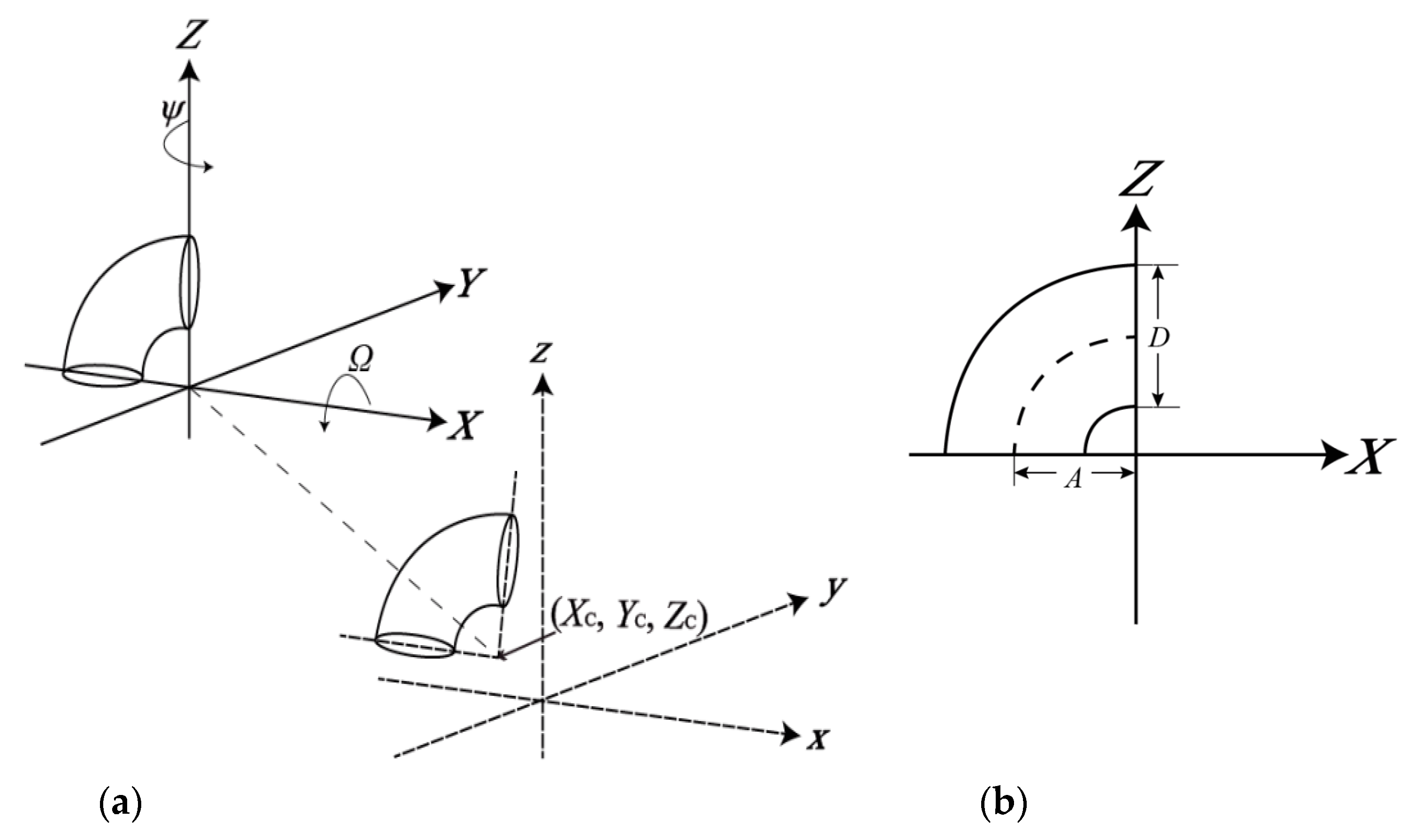
Figure 1.
Parameters of the proposed geometric model of the elbow joint (demonstrated with a 90° short-radius joint): (a) The translational and rotational parameters; (b) The dimensional parameters.
Figure 1.
Parameters of the proposed geometric model of the elbow joint (demonstrated with a 90° short-radius joint): (a) The translational and rotational parameters; (b) The dimensional parameters.
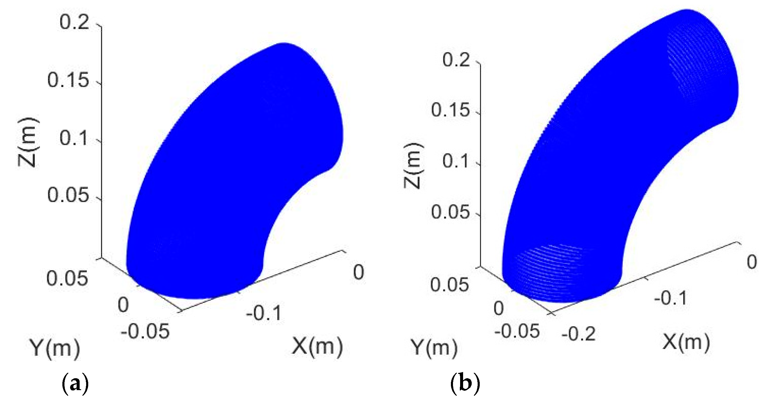
Figure 2.
Simulated point clouds: (a) The short-radius 90° elbow joint; and (b) The long-radius 90° elbow joint.
Figure 2.
Simulated point clouds: (a) The short-radius 90° elbow joint; and (b) The long-radius 90° elbow joint.
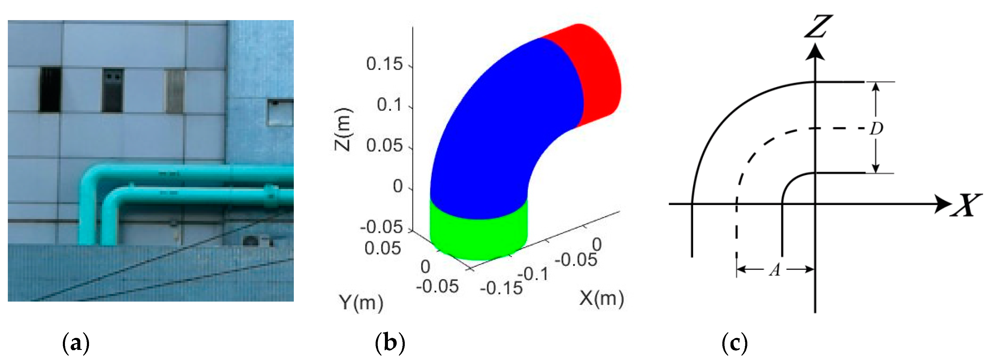
Figure 3.
A joint and its connected pipes: (a) Examples of joints that are indifferentiable from the connected pipe found in Tsuen Wan, Hong Kong, China. (b) Simulated joints with indifferentiable connected cylindrical portions (blue is the bending portion; red and green represent the horizontal and vertical cylindrical portions, respectively); (c) dimensional parameters of the adapted model.
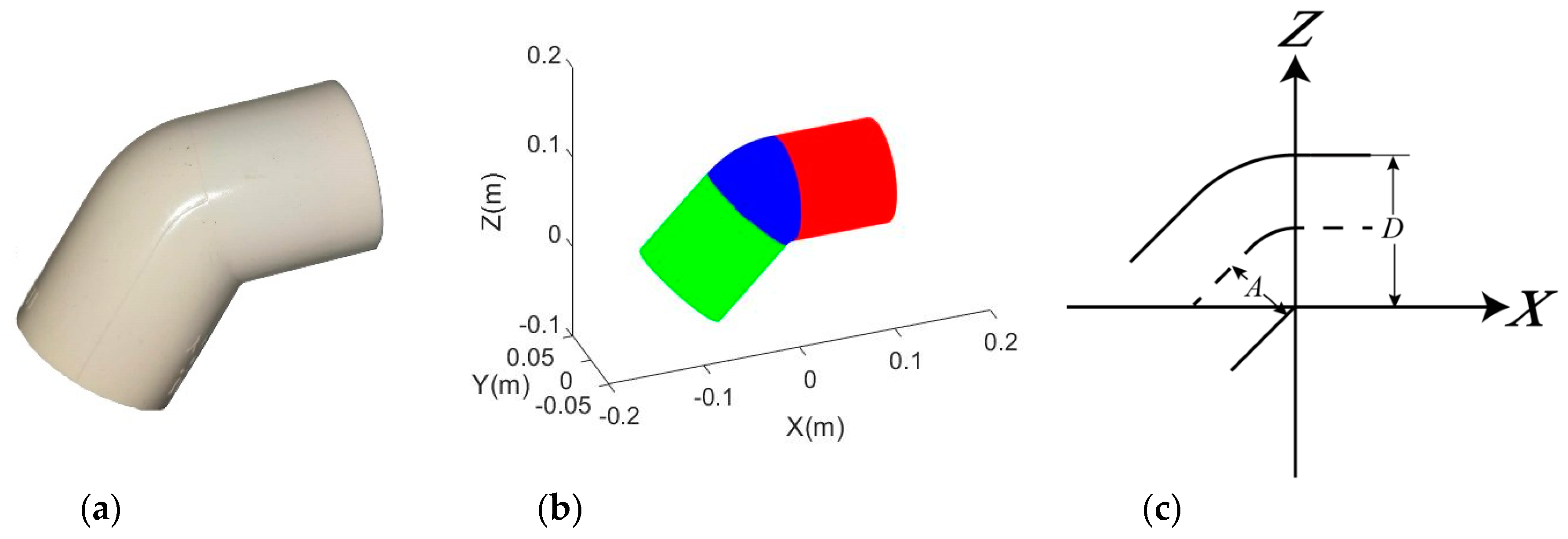
Figure 4.
45° elbow joint: (a) Real example of a plastic 45° elbow joint; (b) Simulated 45° elbow joint (blue is the bending portion; red and green indicate the horizontal and vertical (tilted) cylindrical portions, respectively); (c) Dimensional parameters of the adapted model.
Figure 4.
45° elbow joint: (a) Real example of a plastic 45° elbow joint; (b) Simulated 45° elbow joint (blue is the bending portion; red and green indicate the horizontal and vertical (tilted) cylindrical portions, respectively); (c) Dimensional parameters of the adapted model.
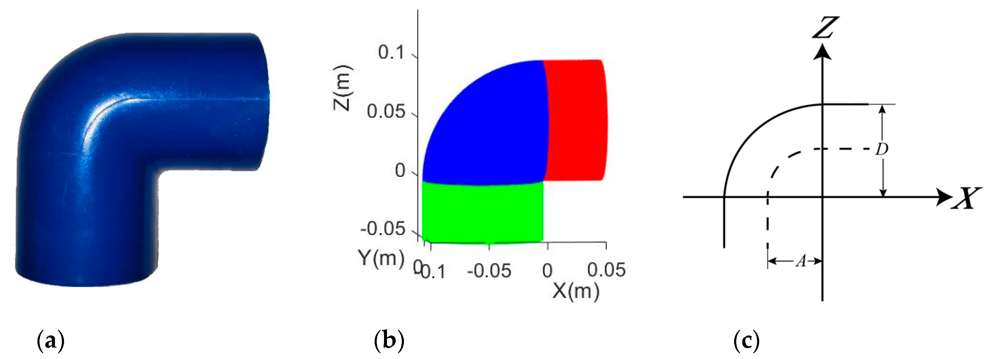
Figure 5.
Shape of a 90° elbow joint: (a) real example of a plastic sharp 90° elbow joint; (b) Simulated sharp 90° elbow joint (blue is the bending portion; red and green represent the horizontal and vertical cylindrical portions, respectively); (c) Dimensional parameters of the adapted model.
Figure 5.
Shape of a 90° elbow joint: (a) real example of a plastic sharp 90° elbow joint; (b) Simulated sharp 90° elbow joint (blue is the bending portion; red and green represent the horizontal and vertical cylindrical portions, respectively); (c) Dimensional parameters of the adapted model.
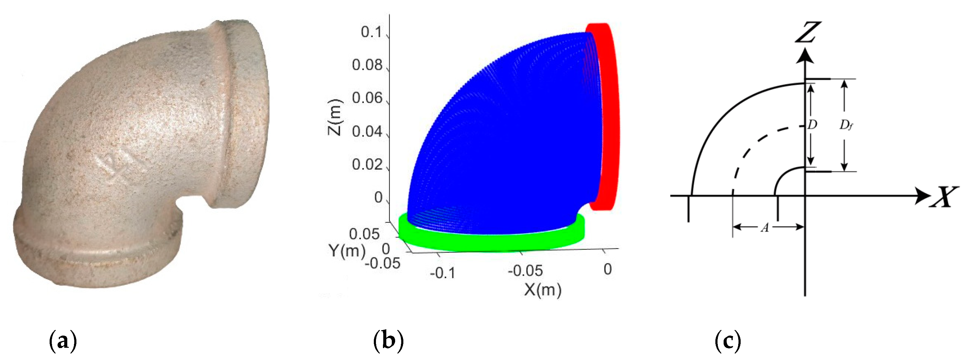
Figure 6.
90° elbow joint with flanges: (a) Real example of an elbow joint with flanges; (b) Simulated elbow joint with flanges (blue is the bending portion; red and green represent the horizontal and vertical flanges, respectively); (c) Dimensional parameters of the adapted model.
Figure 6.
90° elbow joint with flanges: (a) Real example of an elbow joint with flanges; (b) Simulated elbow joint with flanges (blue is the bending portion; red and green represent the horizontal and vertical flanges, respectively); (c) Dimensional parameters of the adapted model.
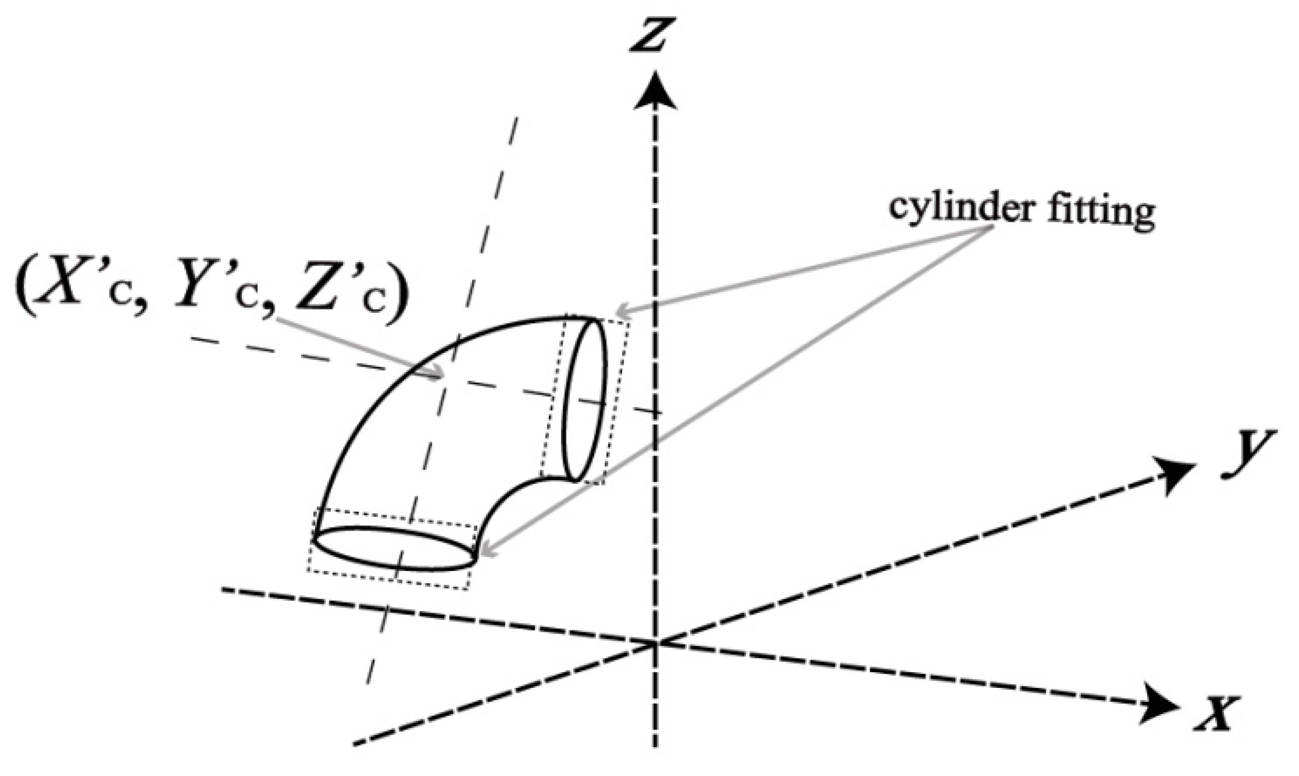
Figure 7.
Computation of the joint inner center using two sets of cylinder fittings.
Figure 7.
Computation of the joint inner center using two sets of cylinder fittings.
Figure 8.
Mounting brackets near two elbow joints found in Yuen Long, Hong Kong, China.
Figure 8.
Mounting brackets near two elbow joints found in Yuen Long, Hong Kong, China.
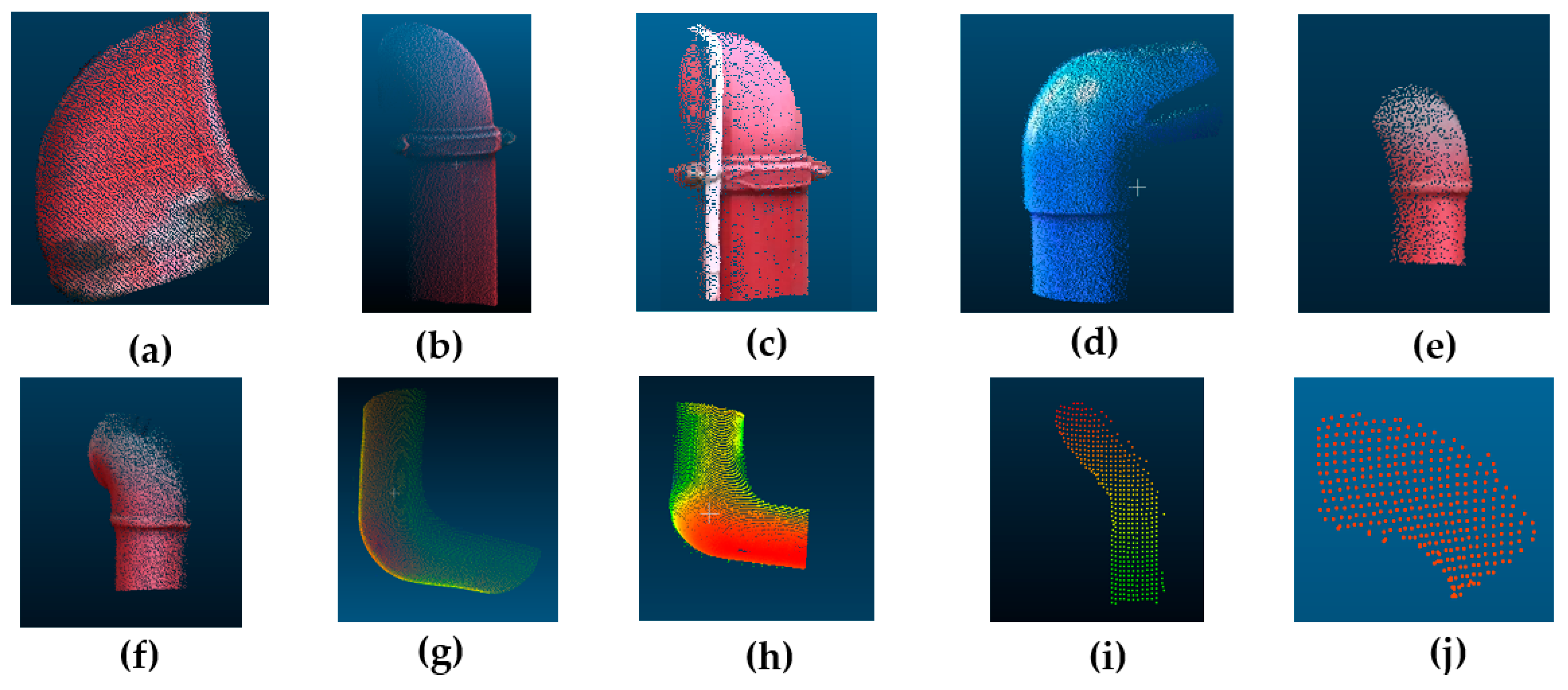
Figure 9.
Real datasets collected by using laser scanners: (a) Joint A; (b) Joint B; (c) Joint C; (d) Joint D; (e) Joint E; (f) Joint F; (g) Joint G; (h) Joint H; (i) Joint I; (j) Joint J.
Figure 9.
Real datasets collected by using laser scanners: (a) Joint A; (b) Joint B; (c) Joint C; (d) Joint D; (e) Joint E; (f) Joint F; (g) Joint G; (h) Joint H; (i) Joint I; (j) Joint J.
Figure 10.
Manual measurement with tape for the circumference (outer diameter) of a joint section.
Figure 10.
Manual measurement with tape for the circumference (outer diameter) of a joint section.
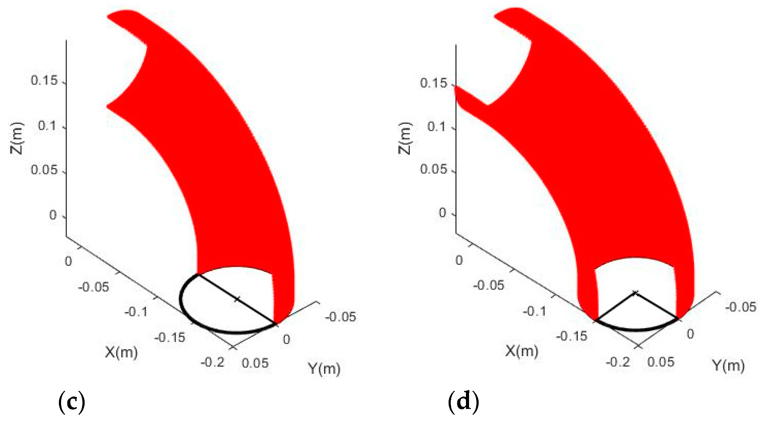
Figure 11.
Simulated joint (Joint (a)) with: (a) 10°, (b) 90°, (c) 180°, and (d) 270° coverage.
Figure 11.
Simulated joint (Joint (a)) with: (a) 10°, (b) 90°, (c) 180°, and (d) 270° coverage.
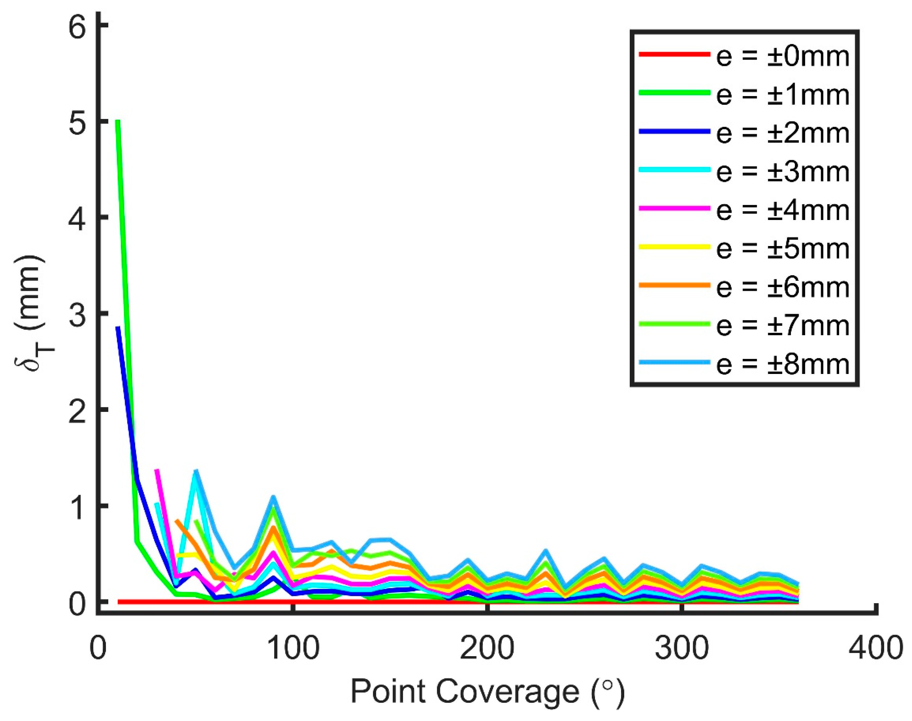
Figure 12.
RMSE of the translational parameters for Joint (a) from 10° to 360° coverage and from noise level 0 mm to ±8 mm.
Figure 12.
RMSE of the translational parameters for Joint (a) from 10° to 360° coverage and from noise level 0 mm to ±8 mm.
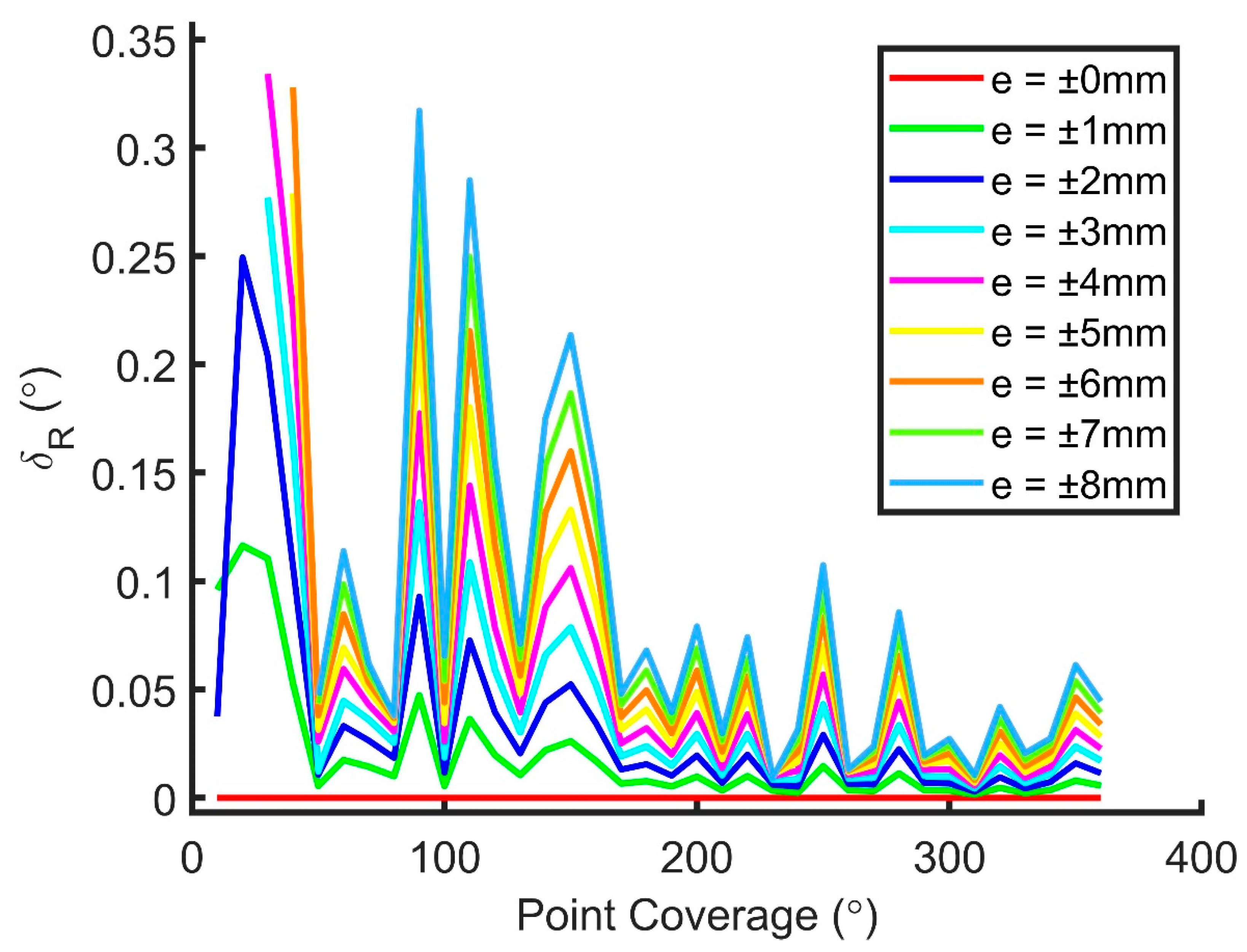
Figure 13.
RMSE of the rotational parameters for Joint (a) from 10° to 360° coverage and from noise level 0 mm to ±8 mm.
Figure 13.
RMSE of the rotational parameters for Joint (a) from 10° to 360° coverage and from noise level 0 mm to ±8 mm.
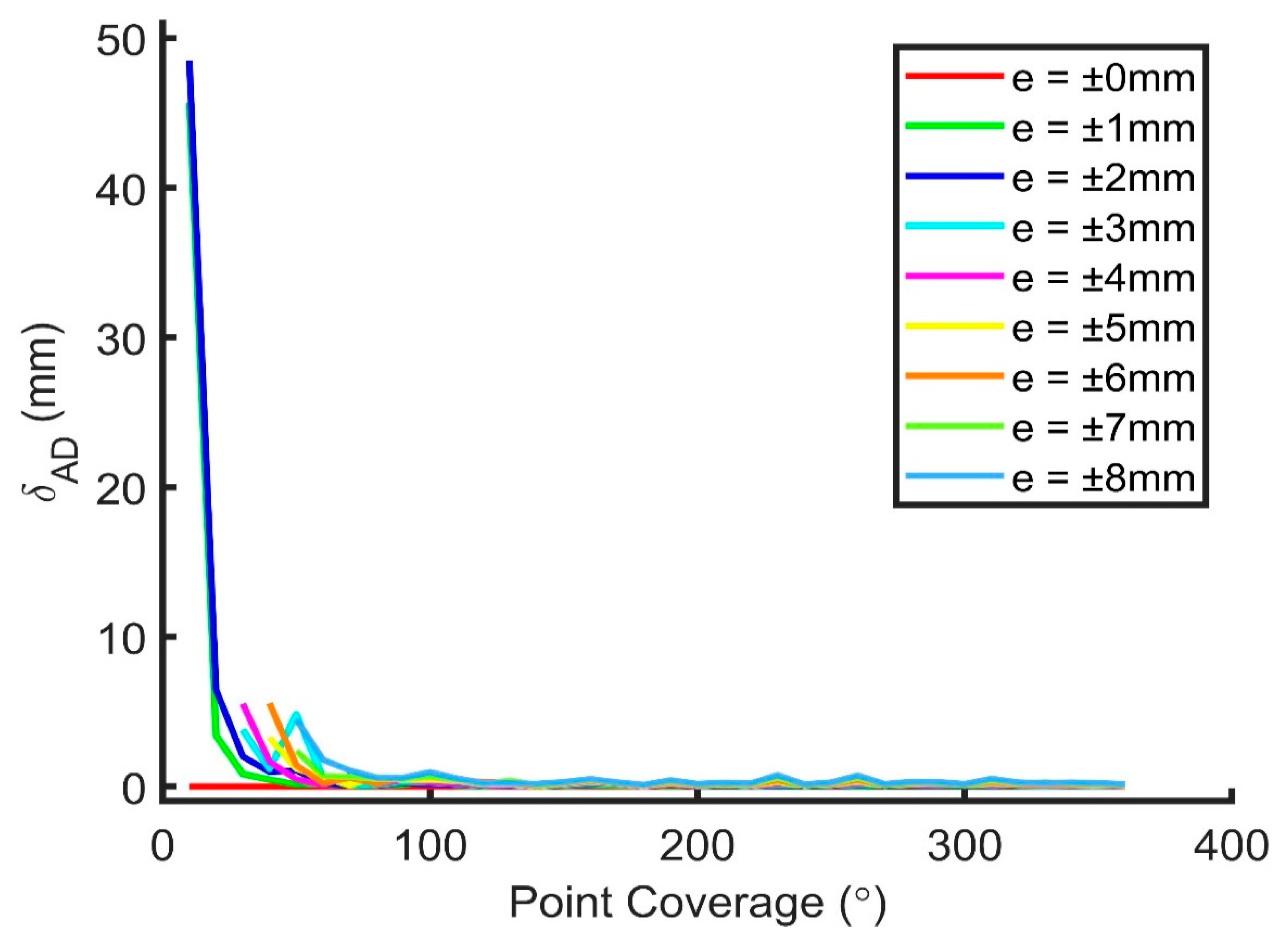
Figure 14.
RMSE of the dimensional parameters for Joint (a) from 10° to 360° coverage and from noise level 0 mm to ±8 mm.
Figure 14.
RMSE of the dimensional parameters for Joint (a) from 10° to 360° coverage and from noise level 0 mm to ±8 mm.
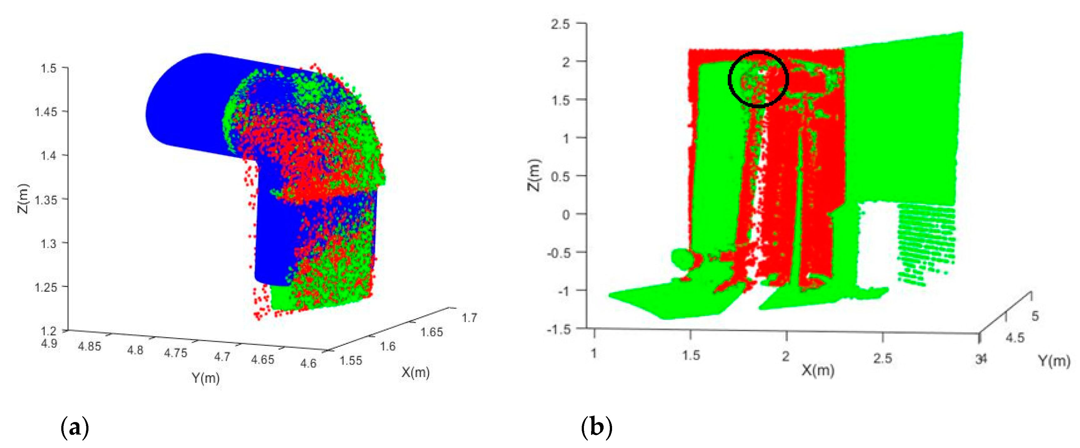
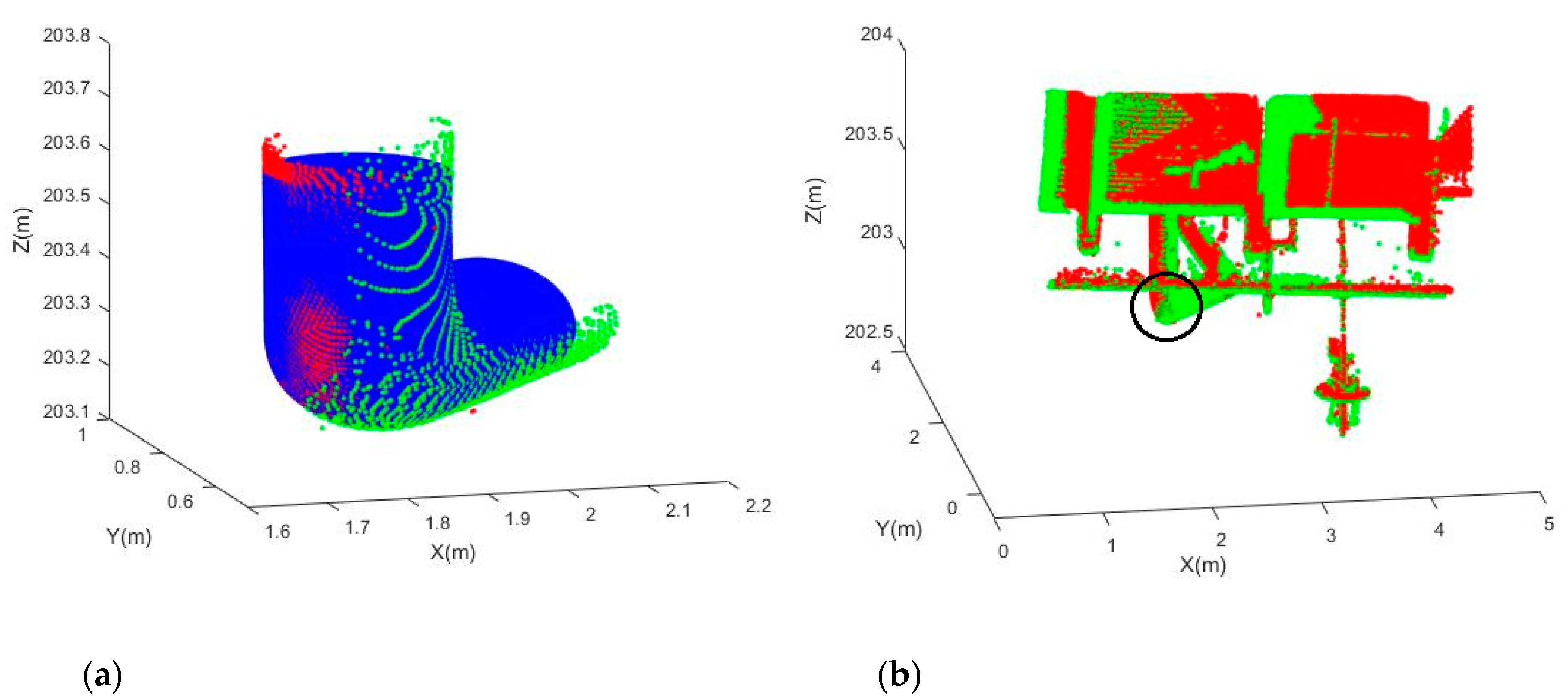
Figure 15.
Registered point clouds: (a) The registered Joints E-F (red for Joint E, green for Joint F, and blue for the model); (b) The entire registered point cloud (the black circle shows the joint position).
Figure 15.
Registered point clouds: (a) The registered Joints E-F (red for Joint E, green for Joint F, and blue for the model); (b) The entire registered point cloud (the black circle shows the joint position).
Figure 16.
Registered point clouds: (a) The registered Joints G-H (red for Joint G, green for Joint H, and blue for the model); (b) The entire registered point cloud (the black circle shows the joint position).
Figure 16.
Registered point clouds: (a) The registered Joints G-H (red for Joint G, green for Joint H, and blue for the model); (b) The entire registered point cloud (the black circle shows the joint position).
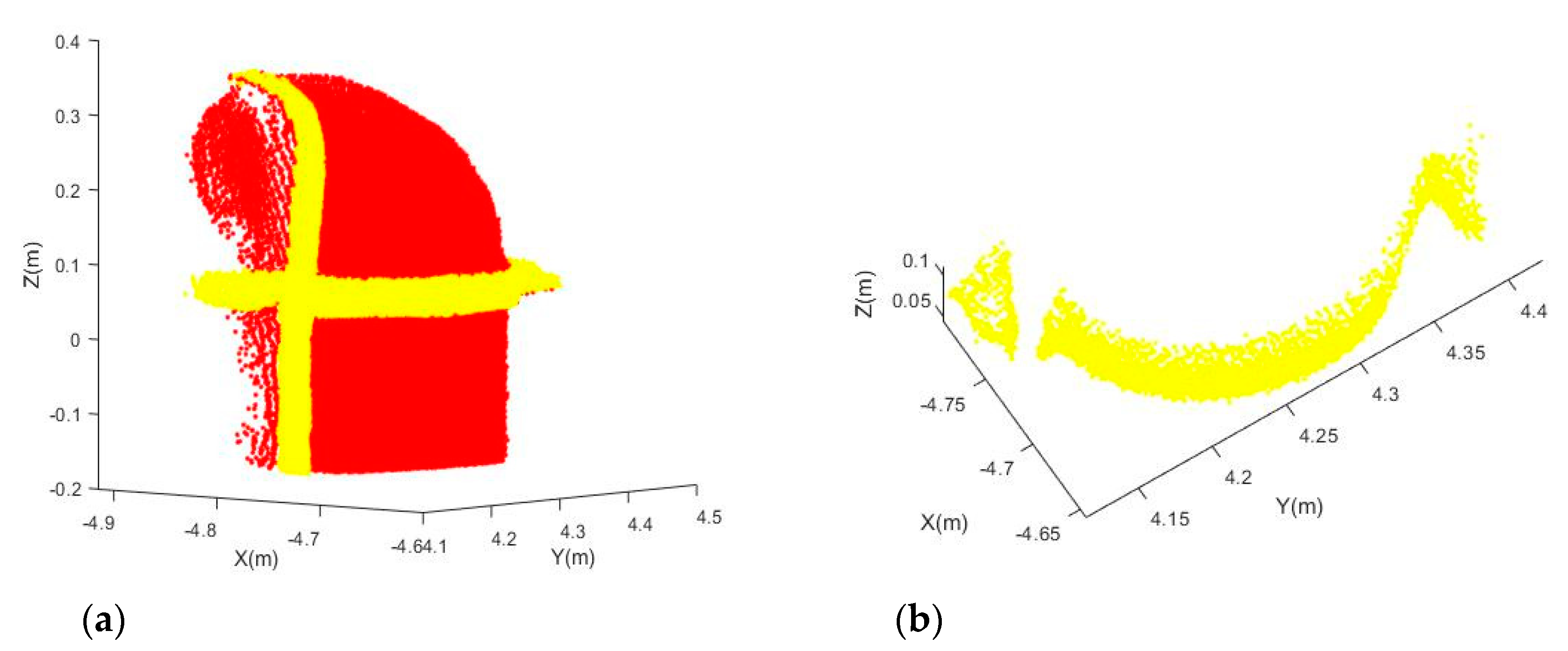
Figure 17.
Detected mounting bracket from Joint B: (a) Point cloud (red) and points with higher residuals (yellow); (b) Extracted mounting bracket.
Figure 17.
Detected mounting bracket from Joint B: (a) Point cloud (red) and points with higher residuals (yellow); (b) Extracted mounting bracket.
Figure 18.
Detected mounting bracket from Joint C: (a) Point cloud (red) and points with higher residuals (yellow); (b) Extracted mounting bracket.
Figure 18.
Detected mounting bracket from Joint C: (a) Point cloud (red) and points with higher residuals (yellow); (b) Extracted mounting bracket.
Table 1.
Details of the simulated datasets.
Table 1.
Details of the simulated datasets.
| Joint | Type (Degree) | A/D Ratio | Flange |
|---|
| a | 90° | 1D | No |
| b | 90° | 1.5D |
| c | 90° | 0.5D |
| d | 45° | 1D |
| e | 45° | 1.5D |
| f | 45° | 0.5D |
| g | 90° | 1D | Yes |
| h | 45° | 1D |
Table 2.
Details of the real datasets.
Table 2.
Details of the real datasets.
| Joint | Type (Degree) | Flange | Scanner | Application Demo |
|---|
| A | 90° | Yes | Trimble SX 10 | n/a |
| B | 90° | No | Trimble SX 10 | n/a |
| C | 90° | No | Trimble SX 10 | Mounting Bracket Detection |
| D | 90° | Yes | Trimble SX 10 | Mounting Bracket Detection |
| E | 90° | Yes | Trimble SX 10 | Point Cloud Registration |
| F | 90° | Yes | Trimble SX 10 | Point Cloud Registration |
| G | 90° | No | Faro Focus3D | Point Cloud Registration |
| H | 90° | No | Faro Focus3D | Point Cloud Registration |
| I | 45° | No | Faro Focus3D | n/a |
| J | 45° | No | Faro Focus3D | n/a |
Table 3.
RMSE of the translation parameters and the rotational parameters estimated from the fitting of the simulated datasets at noise levels from 0 mm to ±3 mm (D = 0.1 m).
Table 3.
RMSE of the translation parameters and the rotational parameters estimated from the fitting of the simulated datasets at noise levels from 0 mm to ±3 mm (D = 0.1 m).
| Noise Level (mm) | | | 0 | ±1 | ±2 | ±3 |
|---|
| Joint | Type | A/D Ratio | | | | | | | | |
| a | 90° | 1D | 0 | 0 | 0 | 0.007 | 0 | 0.012 | 0 | 0.006 |
| b | 90° | 1.5D | 0 | 0 | 0 | 0.012 | 0 | 0.027 | 0.1 | 0.008 |
| c | 90° | 0.5D | 0 | 0 | 0.1 | 0.014 | 0 | 0.002 | 2.4 | 4.007 |
| e | 45° | 1D | 0 | 0 | 0.1 | 0.012 | 0.1 | 0.016 | 0.1 | 0.132 |
| f | 45° | 1.5D | 0 | 0 | 0 | 0.005 | 0.2 | 0.097 | 0.4 | 0.101 |
| g | 45° | 0.5D | 0 | 0 | 0.2 | 0.033 | 0.2 | 0.052 | 1.9 | 3.090 |
| h | 90° | 1D | 0 | 0 | 0 | 0.012 | 0.2 | 0.042 | 0.2 | 0.044 |
| i | 45° | 1D | 0 | 0 | 0.2 | 0.013 | 0.6 | 0.127 | 0.8 | 0.020 |
Table 4.
RMSE of the translation parameters and the rotational parameters estimated from the fitting of the simulated datasets at noise levels from ±3 mm to ±6 mm (D = 0.2 m).
Table 4.
RMSE of the translation parameters and the rotational parameters estimated from the fitting of the simulated datasets at noise levels from ±3 mm to ±6 mm (D = 0.2 m).
| Noise Level (mm) | | | ±3 | ±4 | ±5 | ±6 |
|---|
| Joint | Type | A/D Ratio | | | | | | | | |
| a | 90° | 1D | 0.1 | 0.027 | 0.1 | 0.031 | 0.1 | 0.037 | 0.2 | 0.023 |
| b | 90° | 1.5D | 0 | 0.025 | 0 | 0.015 | 0.2 | 0.087 | 0.1 | 0.024 |
| c | 90° | 0.5D | 0.3 | 0.045 | 1 | 0.181 | n/a | n/a | n/a | n/a |
| e | 45° | 1D | 0.3 | 0.064 | 0.5 | 0.108 | 0.6 | 0.240 | 1.9 | 0.011 |
| f | 45° | 1.5D | 0.5 | 0.017 | 1 | 0.125 | 0.5 | 0.141 | 1.1 | 0.500 |
| g | 45° | 0.5D | 1.7 | 1.772 | 3.7 | 3.082 | n/a | n/a | n/a | n/a |
| h | 90° | 1D | 0.1 | 0.013 | 0.2 | 0.045 | 00.2 | 0.027 | 0.4 | 0.029 |
| i | 45° | 1D | 0.2 | 0.033 | 1.2 | 0.024 | 2 | 0.136 | 2.5 | 0.331 |
Table 5.
RMSE of the dimensional parameters estimated from the fitting of the simulated datasets from 0 mm to ±6 mm (D = 0.2 m).
Table 5.
RMSE of the dimensional parameters estimated from the fitting of the simulated datasets from 0 mm to ±6 mm (D = 0.2 m).
| Noise Level (mm) | | | 0 | ±3 | ±4 | ±5 | ±6 |
|---|
| Joint | Type | A/D Ratio | | | | | |
| a | 90° | 1D | 0 | 0 | 0 | 0 | 0.1 |
| b | 90° | 1.5D | 0 | 0.1 | 0 | 0.1 | 0.2 |
| c | 90° | 0.5D | 0 | 0.2 | 0.3 | n/a | n/a |
| e | 45° | 1D | 0 | 0.4 | 0.1 | 0.5 | 0.3 |
| f | 45° | 1.5D | 0 | 0.1 | 0 | 0.1 | 0.2 |
| g | 45° | 0.5D | 0 | 0.7 | 1.6 | n/a | n/a |
| h | 90° | 1D | 0 | 0.2 | 0.3 | 0.3 | 0.4 |
| i | 45° | 1D | 0 | 0.8 | 0.8 | 0.9 | 1.3 |
Table 6.
RMSE of the dimensional parameters estimated from the fitting of the simulated datasets from ±20 mm to ±80 mm (D = 0.2 m).
Table 6.
RMSE of the dimensional parameters estimated from the fitting of the simulated datasets from ±20 mm to ±80 mm (D = 0.2 m).
| Noise Level (mm) | | | ±20 | ±40 | ±60 | ±80 |
|---|
| Joint | Type | A/D Ratio | | | | | | | | |
| b | 90° | 1.5D | 0.3 | 0.064 | 1.4 | 0.266 | 1.7 | 0.251 | 1.1 | 1.072 |
| f | 45° | 1.5D | 0.8 | 0.171 | n/a | n/a | n/a | n/a | n/a | n/a |
Table 7.
Least-squares estimates and the precision of Joints (a) and (d) with different coverage values.
Table 7.
Least-squares estimates and the precision of Joints (a) and (d) with different coverage values.
| Joint | Type | A/D Ratio | Point Coverage | No. of Points | | | |
|---|
| | | | 90° (25%) | 11,790 | 682.500 | 45.697 | 75.000 |
| | | | | 9.54 × 10⁻² | 6.29 × 10⁻² | 1.14 × 10⁻¹ |
| | | | 180° (50%) | 25,380 | 682.500 | 45.697 | 75.000 |
| | | | | | 5.30 × 10⁻² | 3.68 × 10⁻² | 4.12 × 10⁻² |
| a | 90° | 1D | 270° (75%) | 35,370 | 682.500 | 45.697 | 75.000 |
| | | | | | 4.27 × 10⁻² | 3.05 × 10⁻² | 3.12 × 10⁻² |
| | | | 360° (100%) | 47,160 | 682.500 | 45.697 | 75.000 |
| | | | | | 3.67 × 10⁻² | 2.62 × 10⁻² | 2.62 × 10⁻² |
| | | | 90° (25%) | 11,790 | 601.678 | 45.346 | 75.000 |
| | | | | | 3.25 × 10⁻¹ | 6.29 × 10⁻² | 3.56 × 10⁻¹ |
| | | | 180° (50%) | 25,380 | 601.678 | 45.346 | 75.000 |
| d | 45° | 1D | | | 2.19 × 10⁻¹ | 3.68 × 10⁻² | 1.88 × 10⁻¹ |
| | | | 270° (75%) | 35,370 | 601.678 | 45.346 | 75.000 |
| | | | | | 1.78 × 10⁻¹ | 3.05 × 10⁻² | 1.51 × 10⁻¹ |
| | | | 360° (100%) | 47,160 | 601.678 | 45.346 | 75.000 |
| | | | | | 1.54 × 10⁻¹ | 2.62 × 10⁻² | 1.30 × 10⁻¹ |
Table 8.
Mean least-squares estimates and the precision of Joints A to J.
Table 8.
Mean least-squares estimates and the precision of Joints A to J.
| Joint | Type | No. of Points |
|
|
|
|---|
| A | 90° | 18,966 | 5619.1 | 149.131 | 69.2 |
| | | 7.50 × 10⁻² | 5.16 × 10⁻² | 6.04 × 10⁻² |
| B | 90° | 49,742 | 4391.4 | 103.613 | 129.1 |
| | | | 4.79 × 10⁻² | 7.62 × 10⁻³ | 4.34 × 10⁻² |
| C | 90° | 29,155 | 1350.9 | 111.162 | 114.8 |
| | | | 8.66 × 10⁻² | 3.10 × 10⁻² | 7.68 × 10⁻² |
| D | 90° | 22,223 | 1638.4 | 15.757 | 61.0 |
| | | | 5.97 × 10⁻² | 2.53 × 10⁻² | 5.31 × 10⁻² |
| E | 90° | 8624 | 2583.376 | 42.562 | 49.2 |
| | | | 1.45 × 10⁻¹ | 6.46 × 10⁻² | 1.28 × 10⁻¹ |
| F | 90° | 23,085 | 1593.3 | 60.535 | 48.7 |
| | | | 7.90 × 10⁻² | 2.18 × 10⁻² | 6.88 × 10⁻² |
| G | 90° | 15,629 | 6811.9 | 65.881 | 89.9 |
| | | | 5.54 × 10⁻² | 7.27 × 10⁻³ | 5.65 × 10⁻² |
| H | 90° | 13,569 | 6881.4 | 72.330 | 90.5 |
| | | | 7.11 × 10⁻² | 1.85 × 10⁻² | 6.76 × 10⁻² |
| I | 45° | 7387 | 3163.8 | 35.752 | 75.3 |
| | | | 1.12 × 10⁻¹ | 2.31 × 10⁻² | 7.11 × 10⁻¹ |
| J | 45° | 2356 | 6202.8 | 72.526 | 55.6 |
| | | | 7.53 × 10⁻¹ | 1.98 × 10⁻¹ | 9.82 × 10⁻¹ |
Table 9.
Translation and rotational errors for the registrations.
Table 9.
Translation and rotational errors for the registrations.
| Registration | Joint | | |
|---|
| 1 | E-F | 27 | 1.89 |
| 2 | G-H | 3.8 | 0.36 |

 ,
, 


