Understanding Smartwatch Battery Utilization in the Wild

 , , , ,
Abstract
1. Introduction
2. Related Work
2.1. Smartphone Battery Utilization
2.2. Smartwatch and Other Wearable Device Battery Utilization
2.3. Deep Learning Models for Battery-Powered Devices
3. Methods
3.1. Dataset
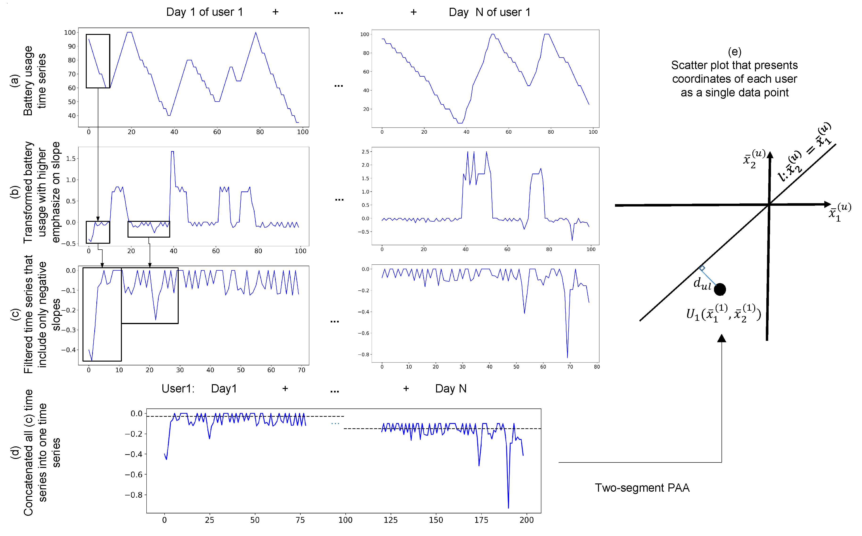
3.2. Finding Common Patterns
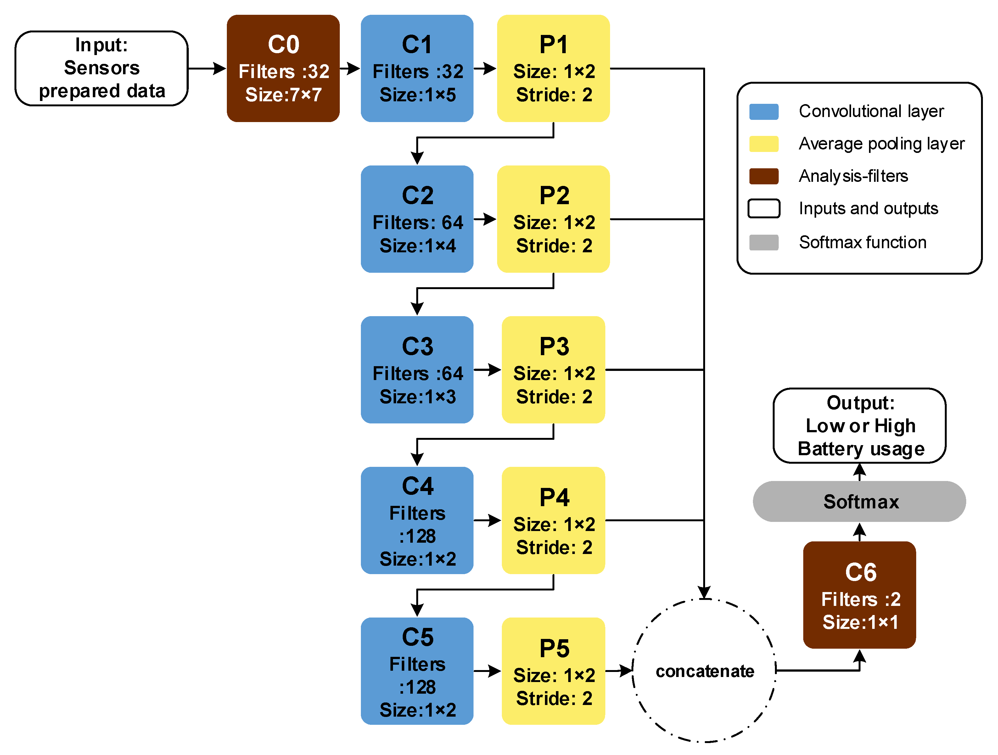
3.3. Fully Convolutional Neural Network (FCNN) Model
3.3.1. Time Alignment
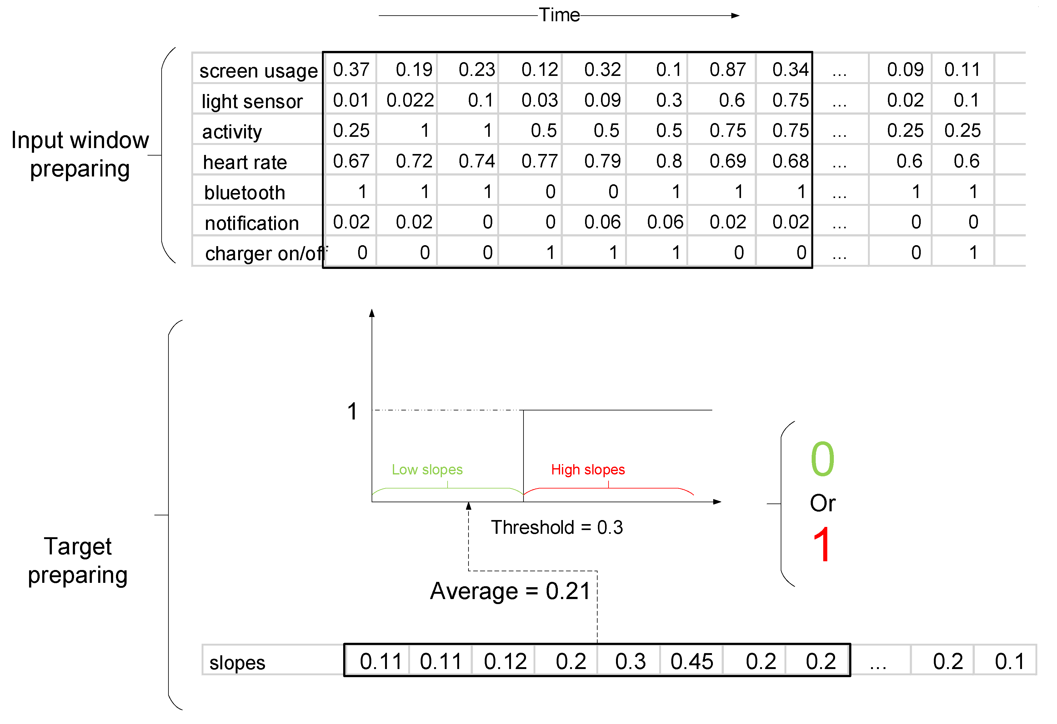
3.3.2. Label Preparation
3.3.3. Input Preparation for the Model
3.3.4. Training Phase
3.3.5. Rationale for Introducing a Customized FCNN Model
3.4. Indexing Battery Performance
4. Results
4.1. Patterns of Battery Drain Identified from Clustering
4.2. Results of the Deep Learning Model
Evaluation of the Deep Learning Model
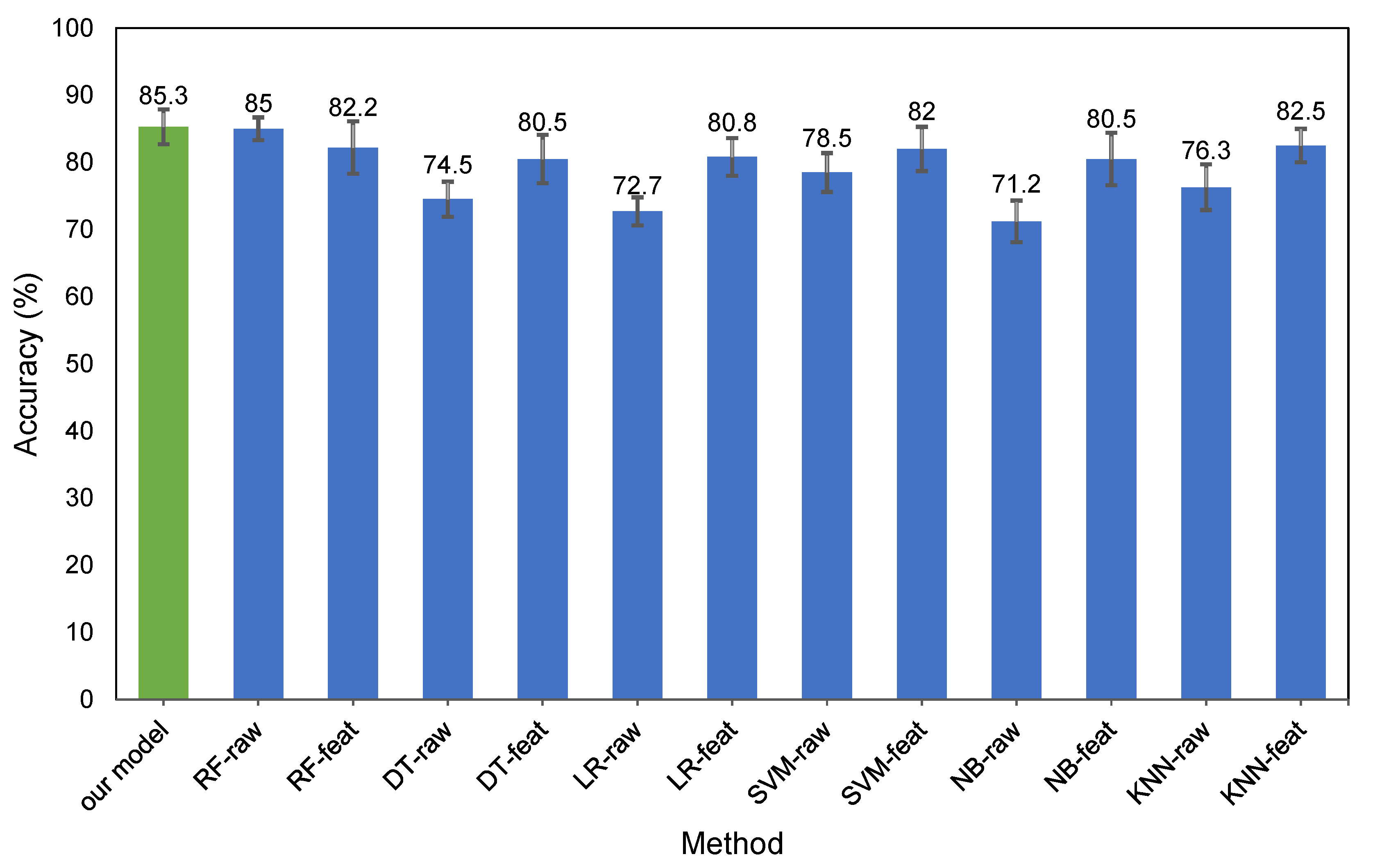
4.3. Comparison with Other Methods
4.4. Filter Exploration of the Deep Learning Model
4.5. Indexing Battery Performance Results
5. Discussion
5.1. Advantages of a Deep Learning Model
- First, we need to have an automatic feature extractor based on battery usage, and the most common method is to use CNN. The lower number of parameters of FCNN versus the CNN and multilayer perceptron (MLP) pair lead us to favor FCNN.
- To extract information for the model to learn, we use limited filters of the first and last layers of our model. This functionality cannot be achieved for other models (e.g., RF) that have similar performance in their final decision.
- Residual connections help us to improve the performance of the model by mixing different levels of features to make the final decision.
- By using a binary classification, we can identify whether the extracted information is related to high or low peaks of battery usage. However, other classification methods, such as regression or multiclass classification, cannot identify such a relation. For example, if we use 10-class classification and choose 1 to be the lowest battery usage and 10 to be the highest battery usage, features that are extracted might be related to two low battery usage classes (e.g., 1, 2 and 3). However, we need only high and low battery users (binary selection) and not multiple classes for the selection.
5.2. Findings and Recommendations
- Devices with newer versions (than 7.1.1) of the Wear OS operating system drain the battery faster than previous versions. Table 10 shows that installing newer versions of Wear OS on the same device causes a deterioration in the battery quality of the device. This could be due to the advances and increase in the number of applications available for smartwatches. All smartwatch devices—without exception—receive updates both from their vendors and Google as an operating system provider. Besides, the number of installed applications does not significantly increase or decrease. Therefore, the number of applications do not play a role in battery discharge.
- Motorola and Sony smartwatch software updates improve battery life, while the battery life of other brands in our dataset deteriorates when updated. Based on the results in Table 10, Sony and Motorola smartwatches have the longest sustainable battery discharge rate, which improved during their lifetime. This illustrates that these two particular brands most likely invest in improvements to their background services and smartwatch skins with the aim of better energy efficiency. Our dataset does not include all existing brands; thus, we cannot claim that this finding is generalizable among all brands.
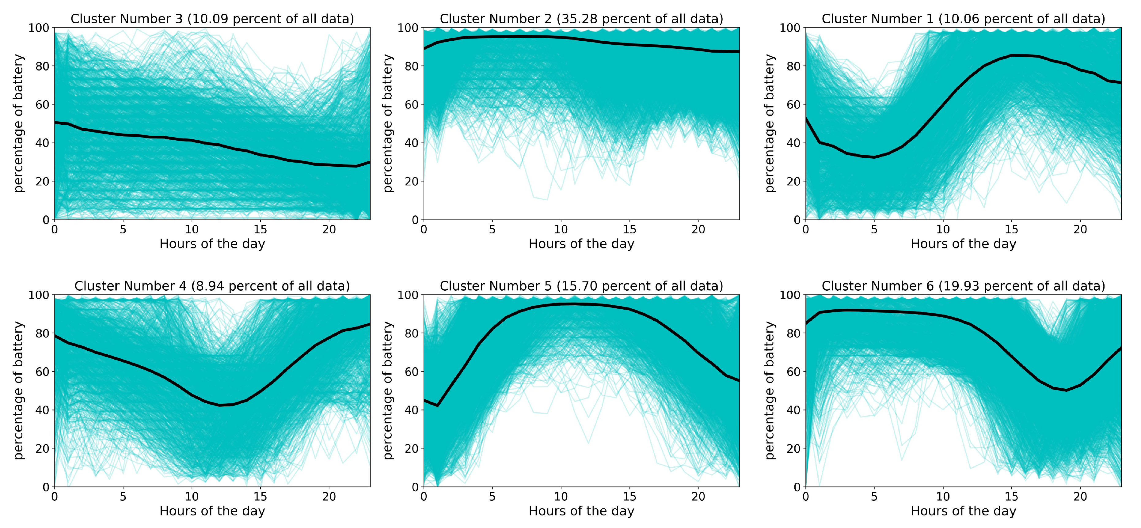
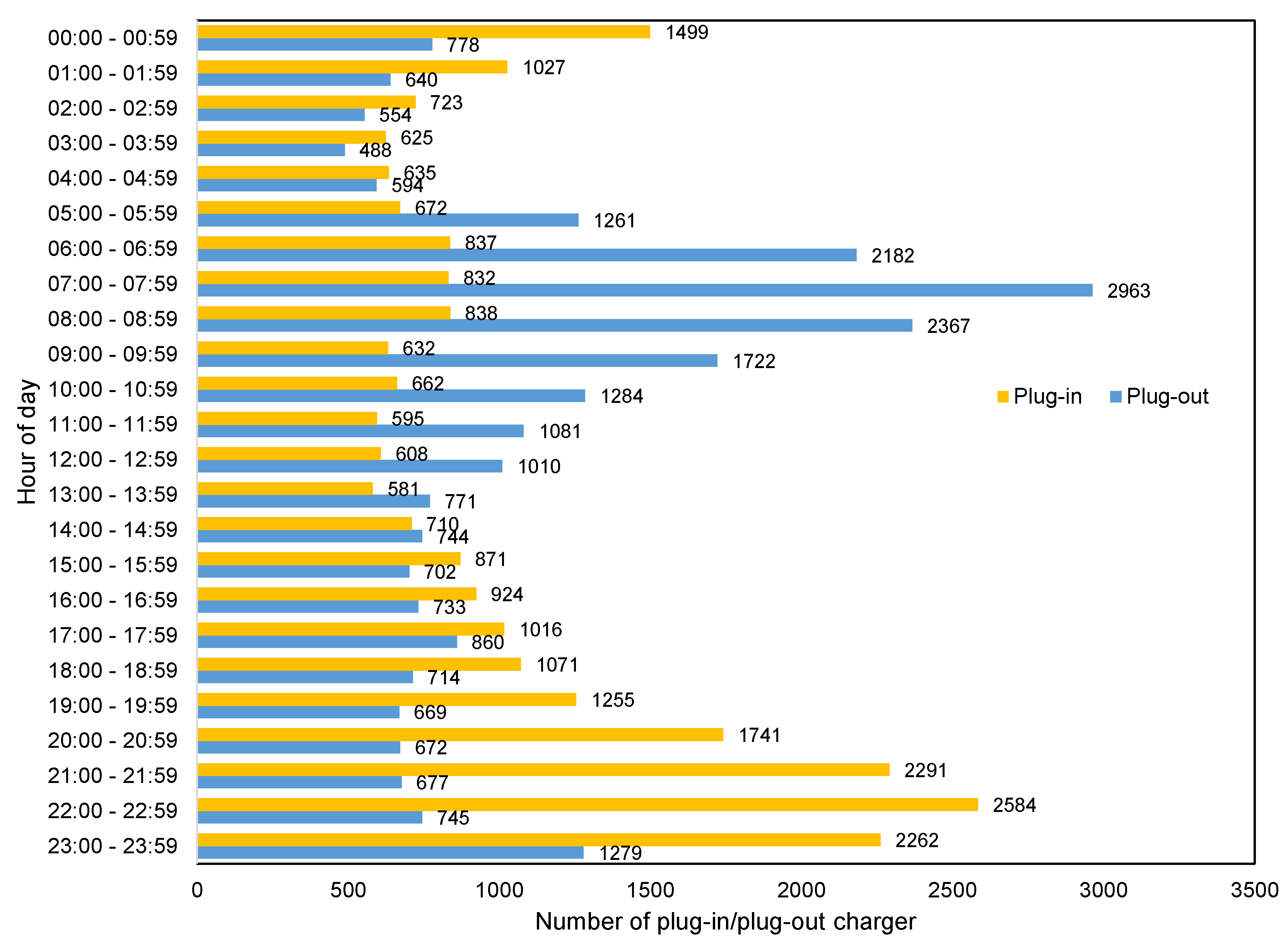
- The highest peak of smartwatch battery drain is during working hours, from 9:00 to 17:00. On the other hand, sleep time, 22:00 to 6:00, is the best time for batch operations on devices, as most users plug their device in to charge for the longest period of time. Cluster 5 and cluster 2 in Figure 4, which account for more than half of users, show that battery usage increases sharply from morning to evening. The behavior of 15.70% of users (cluster 5 in Figure 4) is similar to cluster 2 but with steeper slopes. Other clusters (1, 3 and 4), which account for 29.09% of all users, have different patterns caused by non-routine days. On the other hand, cluster 6 in Figure 4 shows that approximately 19.93% of users charge their device during the last hours of the day and the first hours of the next day and unplug their device before sleeping. Clusters 3, 4 and 6, which represent about 40% of users, show that most smartwatch users connect their device to a charger at bedtime (i.e., at the end of the day or during the first hours of the day) and remove their device from the charger when they wake-up. Figure 5 shows that most users prefer to plug-in their device during the last hours (before sleeping) and unplug their device in the morning (after waking up). This confirms the result of Figure 3, which illustrates the charging patterns of most users. Based on this pattern, we can recommend that batch jobs, such as backing up data to the Cloud or application updates, which require a great deal of battery power, can be performed during sleeping hours.
- Different charging behaviors are observed on weekends compared to weekdays. Figure 4 shows that there is a difference between Saturday and other days of the week. To evaluate this result, we utilize the results of all users’ data who plugged-in for 7 days of the week. By applying a one-way ANOVA statistical test [66], we found that there is a significant difference between Saturday and other days of the week with a p-value < 0.05. A justification for why only Saturday and not Sunday was considered could be due to countries that count Sunday as a working day, such as some countries in the Middle East and North Africa, which biases our results toward Saturday.
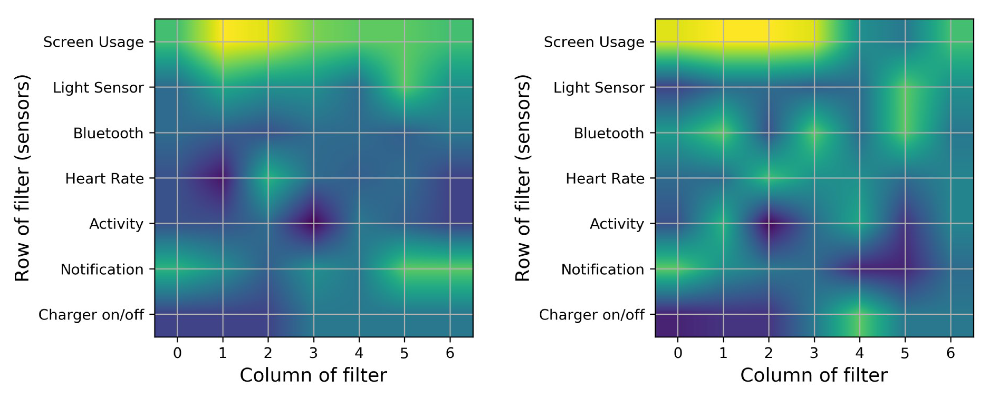
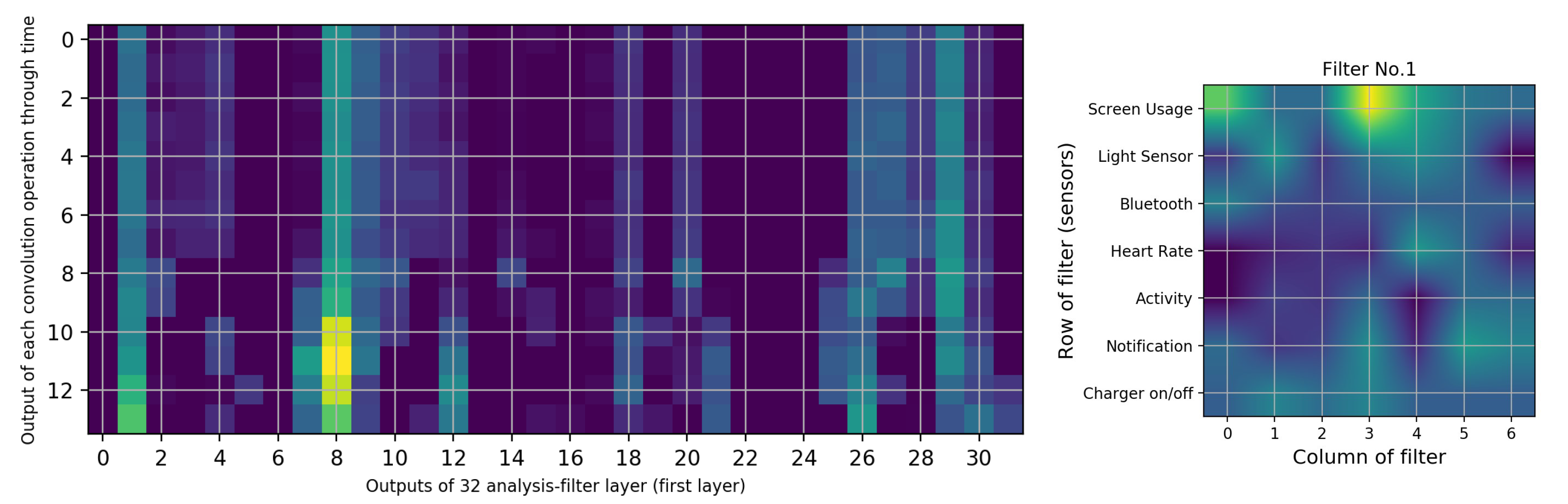
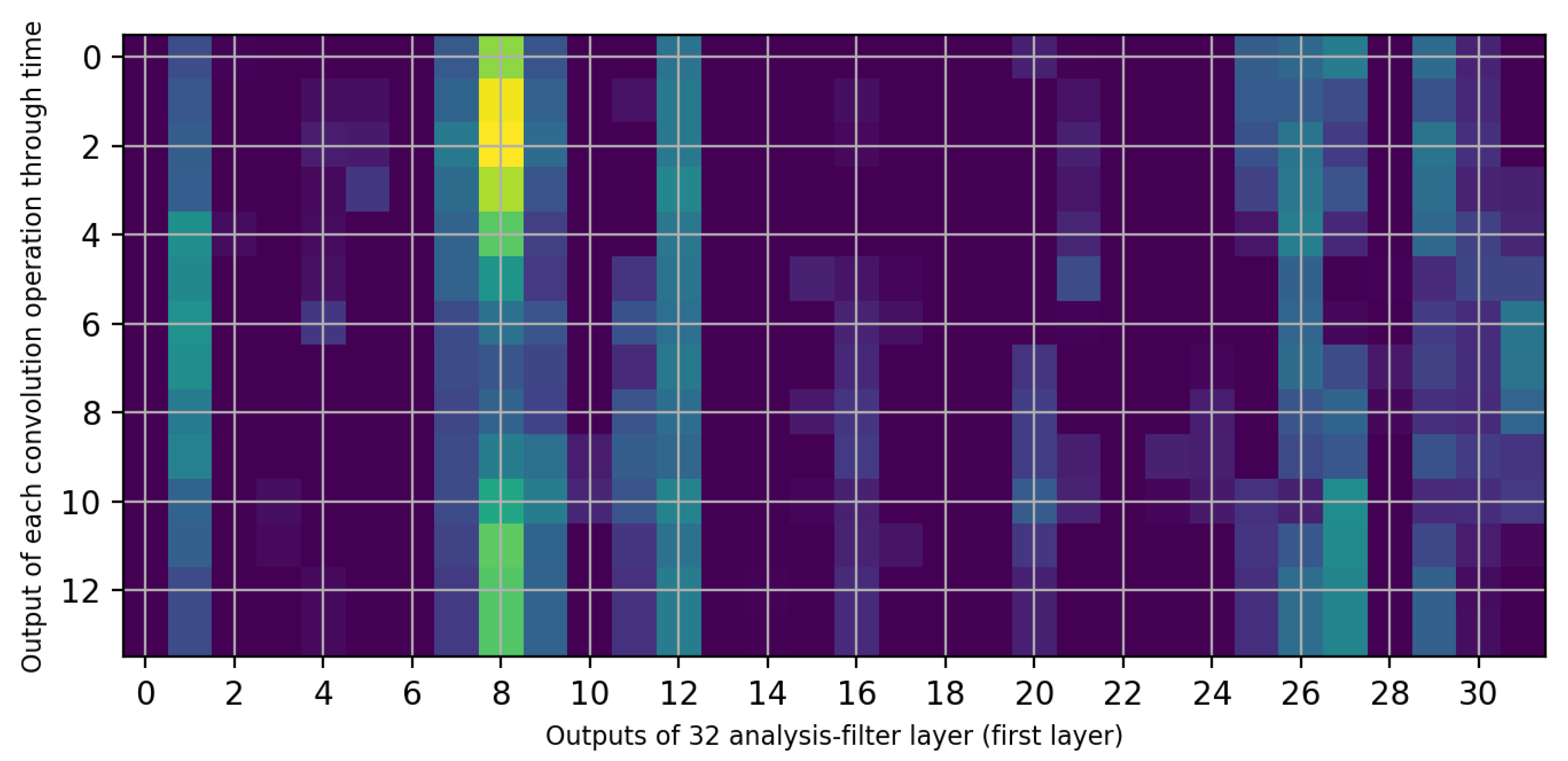
- Interaction with the screen and notifications are the most common causes of battery drain. Based on the results presented in Table 8, we identify that screen usage and notification sensors had more of an impact on battery discharge in comparison to other sensors. The heat map presented in Figure 8 shows that this filter extracts features with most focus on physical activity and Bluetooth, then on heart-rate and then on connection to the charger (which turns on the screen automatically).
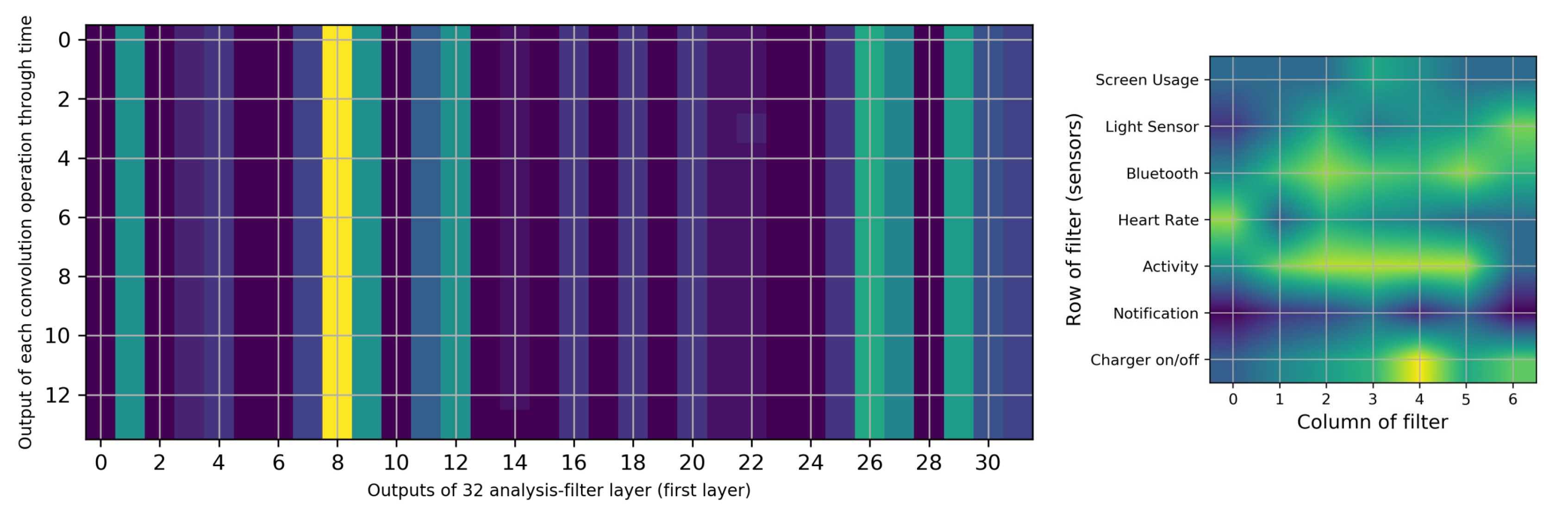
- When users are physically inactive, there is more battery utilization than during physical activities or when inside a vehicle. The effect of turning the charger on/off can be seen in column 8 of Figure 8. When the charger is connected, the model does not consider any other condition. The screen sensor is on average in its maximum state. The Bluetooth sensor is “on” for all of these periods. The heart rate is constant and at an average which is natural. The light sensor increases to its average of all data of light sensors. In addition to the effect of the charger, the activity type is also correlated; the screen, light, heart rate, and Bluetooth show no related changes. The notification sensor is not important for filter 8 based on Figure 9. Among the four types of activities that the Google service can identify, when the user is inactive, more battery consumption is present than in other states. This finding might appear obvious, but it is important to note that earlier versions of smartwatches have strong false positives with wrist movement and automatically turn on the screen [68]; for example, while the user is driving, moving the steering wheel causes the smartwatch to turn on the screen and thus to drain the battery. Our analyses reveals that this problem has been resolved (More details are available in Appendix C).
6. Conclusions and Future Work
Author Contributions
Funding
Conflicts of Interest
Appendix A
| Algorithm A1: Time alignment of all sensors with one reference sensor |
 |
Appendix B
Appendix C


References
- Smartwatches—Statistics & Facts. Available online: https://www.statista.com/topics/4762/smartwatches/ (accessed on 10 June 2020).
- Rogers, E.M. Diffusion of Innovations; Simon and Schuster: New York, NY, USA, 2010. [Google Scholar]
- Rawassizadeh, R.; Price, B.A.; Petre, M. Wearables: Has the age of smartwatches finally arrived? Commun. ACM 2015, 58, 45–47. [Google Scholar] [CrossRef]
- Gong, J.; Yang, X.D.; Irani, P. Wristwhirl: One-handed continuous smartwatch input using wrist gestures. In Proceedings of the 29th Annual Symposium on User Interface Software and Technology, Tokyo, Japan, 16–19 October 2016; pp. 861–872. [Google Scholar]
- Liu, X.; Chen, T.; Qian, F.; Guo, Z.; Lin, F.X.; Wang, X.; Chen, K. Characterizing smartwatch usage in the wild. In Proceedings of the 15th Annual International Conference on Mobile Systems, Applications, and Services, Niagara Falls, NY, USA, 19–23 June 2017; pp. 385–398. [Google Scholar]
- Min, C.; Kang, S.; Yoo, C.; Cha, J.; Choi, S.; Oh, Y.; Song, J. Exploring current practices for battery use and management of smartwatches. In Proceedings of the 2015 ACM International Symposium on Wearable Computers, Osaka, Japan, 7–11 September 2015; pp. 11–18. [Google Scholar]
- Khakurel, J.; Knutas, A.; Melkas, H.; Penzenstadler, B.; Fu, B.; Porras, J. Categorization Framework for Usability Issues of Smartwatches and Pedometers for the Older Adults. In International Conference on Universal Access in Human-Computer Interaction; Springer: Cham, Switzerland, 2018; pp. 91–106. [Google Scholar]
- Wearables Are on the Rise. Available online: https://www2.deloitte.com/be/en/pages/technology-media-and-telecommunications/topics/mobile-consumer-survey-2019/wearables.html (accessed on 11 June 2020).
- Ding, N.; Wagner, D.; Chen, X.; Pathak, A.; Hu, Y.C.; Rice, A. Characterizing and modeling the impact of wireless signal strength on smartphone battery drain. ACM SIGMETRICS Perform. Eval. Rev. 2013, 41, 29–40. [Google Scholar] [CrossRef]
- Balaji, R.; Bhavsar, K.; Bhowmick, B.; Mithun, B.; Chakravarty, K.; Chatterjee, D.; Ghose, A.; Gupta, P.; Jaiswal, D.; Kimbahune, S.; et al. A Framework for Pervasive and Ubiquitous Geriatric Monitoring. In International Conference on Human Aspects of IT for the Aged Population; Springer: Cham, Switzerland, 2018; pp. 205–230. [Google Scholar]
- Wang, R.; Chen, F.; Chen, Z.; Li, T.; Harari, G.; Tignor, S.; Zhou, X.; Ben-Zeev, D.; Campbell, A.T. StudentLife: Assessing mental health, academic performance and behavioral trends of college students using smartphones. In Proceedings of the 2014 ACM International Joint Conference on Pervasive and Ubiquitous Computing, Seattle, WA, USA, 13–17 September 2014; pp. 3–14. [Google Scholar]
- Shoaib, M.; Incel, O.D.; Scolten, H.; Havinga, P. Resource consumption analysis of online activity recognition on mobile phones and smartwatches. In Proceedings of the 2017 IEEE 36th International Performance Computing and Communications Conference (IPCCC), San Diego, CA, USA, 10–12 December 2017; pp. 1–6. [Google Scholar]
- Stephanidis, C.; Salvendy, G.; Antona, M.; Chen, J.Y.; Dong, J.; Duffy, V.G.; Fang, X.; Fidopiastis, C.; Fragomeni, G.; Fu, L.P.; et al. Seven HCI Grand Challenges. Int. J. Hum.–Comput. Interact. 2019, 35, 1229–1269. [Google Scholar] [CrossRef]
- Rawassizadeh, R.; Momeni, E.; Dobbins, C.; Gharibshah, J.; Pazzani, M. Scalable daily human behavioral pattern mining from multivariate temporal data. IEEE Trans. Knowl. Data Eng. 2016, 28, 3098–3112. [Google Scholar] [CrossRef]
- Rawassizadeh, R.; Sen, T.; Kim, S.J.; Meurisch, C.; Keshavarz, H.; Mühlhäuser, M.; Pazzani, M. Manifestation of virtual assistants and robots into daily life: Vision and challenges. CCF Trans. Pervasive Comput. Interact. 2019, 1, 163–174. [Google Scholar] [CrossRef]
- Rawassizadeh, R.; Keshavarz, H.; Pazzani, M. Ghost Imputation: Accurately Reconstructing Missing Data of the Off Period. IEEE Trans. Knowl. Data Eng. 2019. [Google Scholar] [CrossRef]
- Rawassizadeh, R.; Tomitsch, M.; Wac, K.; Tjoa, A.M. UbiqLog: A generic mobile phone-based life-log framework. Pers. Ubiquitous Comput. 2013, 17, 621–637. [Google Scholar] [CrossRef]
- Rawassizadeh, R.; Tomitsch, M.; Nourizadeh, M.; Momeni, E.; Peery, A.; Ulanova, L.; Pazzani, M. Energy-efficient integration of continuous context sensing and prediction into smartwatches. Sensors 2015, 15, 22616–22645. [Google Scholar] [CrossRef]
- Rahmati, A.; Zhong, L. Human–battery interaction on mobile phones. Pervasive Mob. Comput. 2009, 5, 465–477. [Google Scholar] [CrossRef]
- Falaki, H.; Mahajan, R.; Kandula, S.; Lymberopoulos, D.; Govindan, R.; Estrin, D. Diversity in smartphone usage. In Proceedings of the 8th International Conference on Mobile Systems, Applications, and Services, San Francisco, CA, USA, 15–18 June 2010; pp. 179–194. [Google Scholar]
- Ferreira, D.; Dey, A.K.; Kostakos, V. Understanding human-smartphone concerns: A study of battery life. In International Conference on Pervasive Computing; Springer: San Francisco, CA, USA, 2011; pp. 19–33. [Google Scholar]
- Athukorala, K.; Lagerspetz, E.; Von Kügelgen, M.; Jylhä, A.; Oliner, A.J.; Tarkoma, S.; Jacucci, G. How carat affects user behavior: Implications for mobile battery awareness applications. In Proceedings of the SIGCHI Conference on Human Factors in Computing Systems, Toronto, ON, Canada, 26 April–1 May 2014; pp. 1029–1038. [Google Scholar]
- Zhang, L.; Tiwana, B.; Qian, Z.; Wang, Z.; Dick, R.P.; Mao, Z.M.; Yang, L. Accurate online power estimation and automatic battery behavior based power model generation for smartphones. In Proceedings of the 8th IEEE/ACM/IFIP International Conference on Hardware/Software Codesign and System Synthesis, Scottsdale, AZ, USA, 24–29 October 2010; pp. 105–114. [Google Scholar]
- Ali, M.; Zain, J.M.; Zolkipli, M.F.; Badshah, G. Mobile cloud computing & mobile battery augmentation techniques: A survey. In Proceedings of the 2014 IEEE Student Conference on Research and Development, Penang, Malaysia, 16–17 December 2014; pp. 1–6. [Google Scholar]
- Chen, X.; Ding, N.; Jindal, A.; Hu, Y.C.; Gupta, M.; Vannithamby, R. Smartphone energy drain in the wild: Analysis and implications. ACM SIGMETRICS Perform. Eval. Rev. 2015, 43, 151–164. [Google Scholar] [CrossRef]
- Perrucci, G.P.; Fitzek, F.H.; Widmer, J. Survey on energy consumption entities on the smartphone platform. In Proceedings of the 2011 IEEE 73rd Vehicular Technology Conference (VTC Spring), Budapest, Hungary, 15–18 May 2011; pp. 1–6. [Google Scholar]
- Peltonen, E.; Lagerspetz, E.; Nurmi, P.; Tarkoma, S. Energy modeling of system settings: A crowdsourced approach. In Proceedings of the 2015 IEEE International Conference on Pervasive Computing and Communications (PerCom), St. Louis, MO, USA, 23–27 March 2015; pp. 37–45. [Google Scholar]
- Lee, U.; Jeong, H.; Kim, H.; Kim, R.; Jeong, Y. Smartwatch Wearing Behavior Analysis: A Longitudinal Study. In ACM International Joint Conference on Pervasive and Ubiquitous Computing (Ubicomp); ACM SIGCHI AND SIGMOBILE: Maui, HI, USA, 2017. [Google Scholar]
- Gartner Survey Shows Wearable Devices Need to Be More Useful. Available online: https://www.gartner.com/en/newsroom/press-releases/2016-12-07-gartner-survey-shows-wearable-devices-need-to-be-more-useful (accessed on 11 June 2020).
- Fadhil, A. Beyond Technical Motives: Perceived User Behavior in Abandoning Wearable Health & Wellness Trackers. arXiv 2019, arXiv:1904.07986. [Google Scholar]
- Dehghani, M.; Kim, K.J. The effects of design, size, and uniqueness of smartwatches: Perspectives from current versus potential users. Behav. Inf. Technol. 2019, 38, 1143–1153. [Google Scholar] [CrossRef]
- Yao, Y.; Liu, X.; Qian, F. Understanding the Predictability of Smartwatch Usage. In Proceedings of the 5th ACM Workshop on Wearable Systems and Applications, Seoul, Korea, 21 June 2019; pp. 11–16. [Google Scholar]
- Poyraz, E.; Memik, G. Analyzing power consumption and characterizing user activities on smartwatches: Summary. In Proceedings of the 2016 IEEE International Symposium on Workload Characterization (IISWC), Providence, RI, USA, 25–27 September 2016; pp. 1–2. [Google Scholar]
- Visuri, A.; Sarsenbayeva, Z.; van Berkel, N.; Goncalves, J.; Rawassizadeh, R.; Kostakos, V.; Ferreira, D. Quantifying sources and types of smartwatch usage sessions. In Proceedings of the 2017 CHI Conference on Human Factors in Computing Systems, Denver, CO, USA, 6–11 May 2017; pp. 3569–3581. [Google Scholar]
- LeCun, Y.; Bengio, Y.; Hinton, G. Deep learning. Nature 2015, 521, 436. [Google Scholar] [CrossRef] [PubMed]
- Graves, A.; Mohamed, A.R.; Hinton, G. Speech recognition with deep recurrent neural networks. In Proceedings of the 2013 IEEE International Conference on Acoustics, Speech and Signal Processing, Vancouver, BC, Canada, 26–31 May 2013; pp. 6645–6649. [Google Scholar]
- Sundermeyer, M.; Schlüter, R.; Ney, H. LSTM neural networks for language modeling. In Proceedings of the Thirteenth Annual Conference of the International Speech Communication Association, Portland, OR, USA, 9–13 September 2012. [Google Scholar]
- Bahdanau, D.; Cho, K.; Bengio, Y. Neural machine translation by jointly learning to align and translate. arXiv 2014, arXiv:1409.0473. [Google Scholar]
- Ordóñez, F.; Roggen, D. Deep convolutional and lstm recurrent neural networks for multimodal wearable activity recognition. Sensors 2016, 16, 115. [Google Scholar] [CrossRef]
- Ronao, C.A.; Cho, S.B. Human activity recognition with smartphone sensors using deep learning neural networks. Expert Syst. Appl. 2016, 59, 235–244. [Google Scholar] [CrossRef]
- Stamate, C.; Magoulas, G.D.; Küppers, S.; Nomikou, E.; Daskalopoulos, I.; Luchini, M.U.; Moussouri, T.; Roussos, G. Deep learning Parkinson’s from smartphone data. In Proceedings of the 2017 IEEE International Conference on Pervasive Computing and Communications (PerCom), Kona, HI, USA, 13–17 March 2017; pp. 31–40. [Google Scholar]
- Mahbub, U.; Sarkar, S.; Patel, V.M.; Chellappa, R. Active user authentication for smartphones: A challenge data set and benchmark results. In Proceedings of the 2016 IEEE 8th International Conference on Biometrics Theory, Applications and Systems (BTAS), Niagara Falls, NY, USA, 6–9 September 2016; pp. 1–8. [Google Scholar]
- Lane, N.D.; Georgiev, P.; Mascolo, C.; Gao, Y. ZOE: A cloud-less dialog-enabled continuous sensing wearable exploiting heterogeneous computation. In Proceedings of the 13th Annual International Conference on Mobile Systems, Applications, and Services, Florence, Italy, 18–22 May 2015; pp. 273–286. [Google Scholar]
- Rawassizadeh, R.; Pierson, T.J.; Peterson, R.; Kotz, D. NoCloud: Exploring network disconnection through on-device data analysis. IEEE Pervasive Comput. 2018, 17, 64–74. [Google Scholar] [CrossRef]
- Bhattacharya, S.; Lane, N.D. From smart to deep: Robust activity recognition on smartwatches using deep learning. In Proceedings of the 2016 IEEE International Conference on Pervasive Computing and Communication Workshops (PerCom Workshops), Sydney, Australia, 14–18 March 2016; pp. 1–6. [Google Scholar]
- Binder, A.; Montavon, G.; Lapuschkin, S.; Müller, K.R.; Samek, W. Layer-wise relevance propagation for neural networks with local renormalization layers. In International Conference on Artificial Neural Networks; Springer: Cham, Switzerland, 2016; pp. 63–71. [Google Scholar]
- Olah, C.; Mordvintsev, A.; Schubert, L. Feature visualization. Distill 2017, 2, e7. [Google Scholar] [CrossRef]
- Zeiler, M.D.; Fergus, R. Visualizing and understanding convolutional networks. In European Conference on Computer Vision; Springer: Cham, Switzerland, 2014; pp. 818–833. [Google Scholar]
- Zhang, Q.; Cao, R.; Shi, F.; Wu, Y.N.; Zhu, S.C. Interpreting cnn knowledge via an explanatory graph. In Proceedings of the Thirty-Second AAAI Conference on Artificial Intelligence, New Orleans, LA, USA, 2–7 February 2018. [Google Scholar]
- Zhang, Q.; Cao, R.; Wu, Y.N.; Zhu, S.C. Growing interpretable part graphs on convnets via multi-shot learning. In Proceedings of the Thirty-First AAAI Conference on Artificial Intelligence, San Francisco, CA, USA, 4–9 February 2017. [Google Scholar]
- Dosovitskiy, A.; Brox, T. Inverting visual representations with convolutional networks. In Proceedings of the IEEE Conference on Computer Vision and Pattern Recognition, San Juan, PR, USA, 26 June–1 July 2016; pp. 4829–4837. [Google Scholar]
- Oppenheim, A.V. Discrete-Time Signal Processing; Prentice-Hall: Saddle River, NJ, USA, 1999. [Google Scholar]
- Rawassizadeh, R.; Dobbins, C.; Akbari, M.; Pazzani, M. Indexing Multivariate Mobile Data through Spatio-Temporal Event Detection and Clustering. Sensors 2019, 19, 448. [Google Scholar] [CrossRef]
- Davis, P.J. Interpolation and Approximation; Dover Publications: Mineola, NY, USA, 1975. [Google Scholar]
- Hagan, M.T.; Demuth, H.B.; Beale, M. Neural Network Design; Martin Hagan, Oklahoma State University: Stillwater, OK, USA, 1997. [Google Scholar]
- Patro, S.; Sahu, K.K. Normalization: A preprocessing stage. arXiv 2015, arXiv:1503.06462. [Google Scholar] [CrossRef]
- LeCun, Y.; Bottou, L.; Bengio, Y.; Haffner, P. Gradient-based learning applied to document recognition. Proc. IEEE 1998, 86, 2278–2324. [Google Scholar] [CrossRef]
- Long, J.; Shelhamer, E.; Darrell, T. Fully convolutional networks for semantic segmentation. In Proceedings of the IEEE Conference on Computer Vision and Pattern Recognition, San Juan, PR, USA, 7–12 June 2015; pp. 3431–3440. [Google Scholar]
- Boureau, Y.L.; Ponce, J.; LeCun, Y. A theoretical analysis of feature pooling in visual recognition. In Proceedings of the 27th International Conference on Machine Learning (ICML-10), Haifa, Israel, 21–24 June 2010; pp. 111–118. [Google Scholar]
- MacQueen, J. Some methods for classification and analysis of multivariate observations. In Proceedings of the Fifth Berkeley Symposium on Mathematical Statistics and Probability; Le Cam, L.M., Neyman, J., Eds.; University of California Press: Berkeley, CA, USA, 1967; Volume 1, pp. 281–297. [Google Scholar]
- Berndt, D.J.; Clifford, J. Using Dynamic Time Warping to Find Patterns in Time Series; KDD Workshop: Seattle, WA, USA, 1994; Volume 10, pp. 359–370. [Google Scholar]
- Rousseeuw, P.J. Silhouettes: A graphical aid to the interpretation and validation of cluster analysis. J. Comput. Appl. Math. 1987, 20, 53–65. [Google Scholar] [CrossRef]
- Maragos, P. Slope transforms: Theory and application to nonlinear signal processing. IEEE Trans. Signal Process. 1995, 43, 864–877. [Google Scholar] [CrossRef]
- Keogh, E.; Chakrabarti, K.; Pazzani, M.; Mehrotra, S. Dimensionality reduction for fast similarity search in large time series databases. Knowl. Inf. Syst. 2001, 3, 263–286. [Google Scholar] [CrossRef]
- Ballantine, J.P.; Jerbert, A.R. Distance from a Line, or Plane, to a Poin. Am. Math. Mon. 1952, 59, 242–243. [Google Scholar] [CrossRef]
- Girden, E.R. ANOVA: Repeated Measures; Sage Publications, Inc.: Thousand Oaks, CA, USA, 1992; Volume 84. [Google Scholar]
- Elliott, D.F. Handbook of Digital Signal Processing: Engineering Applications; Elsevier: Amsterdam, The Netherlands, 2013. [Google Scholar]
- Karatas, C.; Liu, L.; Li, H.; Liu, J.; Wang, Y.; Tan, S.; Yang, J.; Chen, Y.; Gruteser, M.; Martin, R. Leveraging wearables for steering and driver tracking. In Proceedings of the IEEE INFOCOM 2016-The 35th Annual IEEE International Conference on Computer Communications, San Francisco, CA, USA, 10–14 April 2016; pp. 1–9. [Google Scholar]


| Paper | Key Findings |
|---|---|
| Min et al. [6] | - Battery consumption of smartwatches is lower than smartphones - Satisfaction and concerns with smartwatch battery life - Recharging patterns of smartwatches using 17 participants |
| Liu et al. [5] | - Push notifications, CPU, screen and network traffic are important to battery usage |
| Shoaib et al. [12] | - Impact of recognizing smoking task on CPU consumption by using one sensor in one task (recognizing smoking) for the smartwatch |
| Yao et al. [32] | - Predictability of battery usage, application launches and screen display |
| Poyraz and Memik [33] | - Importance of screen and CPU in use of active power - Third-party applications use the battery up to four times more |
| Visuri et al. [34] | - Different behaviors between smartphone and smartwatch users - Notifications and screen sensors are used for their analysis |
| Jeong et al. [28] | - Analyzing temporal wearing patterns of smartwatches - Studying wearing behaviors of smartwatches |
| Sensor Name | Total Number of Data Points (671 Users) | Numbers of Data Points (67 Users) for the Deep Learning Model | Description |
|---|---|---|---|
| Screen usage | 2,340,760 | 489,756 | - Start and end time, when the screen is on or off |
| Heart rate | 380,099 | 101,287 | - Beats per minute (bpm) based on user-defined intervals for recording |
| Bluetooth | 506,545 | 42,822 | - The timestamp for establishing or disconnecting a connection from the smartphone via Bluetooth |
| Ambient light | 1,104,511 | 355,660 | - Ambient illuminance (lux) |
| Activity | 502,176 | 80,948 | - Type of activity (extracted from the Google FIT API) |
| - Activity duration | |||
| Notification | 10,965,195 | 594,157 | - Name and time stamp of the notification package |
| Battery | 2,599,564 | 266,667 | - Battery status in percent |
| - State of charge (charging or discharging) | |||
| Total number | 18,398,850 | 1,931,297 |
| Time Stamp (Original Format) | Fitness Activity | Number of Notifications (Normalized) | Battery Sensor | Bluetooth | Screen Usage (min) | Heart Rate | Light Sensor (lux) |
|---|---|---|---|---|---|---|---|
| 10608291121 | 1 | 0.001 | 56.5 | 1 | 0.13618333 | 71 | 750.167 |
| 10609201429 | 1 | 0.001 | 47.4026 | 0 | 0.0823 | 64 | 86.7037 |
| 10611040931 | 3 | NaN | 72.3096 | 1 | 0.29395 | 97 | 107.556 |
| 11611241736 | 1 | 0.001 | 87.0794 | 1 | 0.07845 | 85 | NaN |
| 11704291950 | 1 | 0.01 | 89.9823 | 1 | 0.07145 | 86 | NaN |
| 14602041950 | 3 | 0.1 | 32.55 | 1 | 0.08293333 | 62 | 5.41002 |
| 18803220806 | 1 | 0.02 | 92.3661 | 1 | 0.01396666 | 83 | 2 |
| 26610211632 | 1 | 10 | 75.6452 | 1 | 0.04478333 | 74 | 153.889 |
| 40702051322 | 4 | 0.01 | 68.0398 | 1 | 0.06195 | 66 | 28.5085 |
| 52706201954 | 1 | NaN | 59.6354 | 1 | 0.3446 | 59 | 2 |
| Region | Users (in Percentage) |
|---|---|
| Europe | 47.17 |
| North America | 40.75 |
| Asia | 10.65 |
| Australia and Ocean | 0.94 |
| South America | 0.16 |
| North Africa | 0.01 |
| Day of Week | Number of Plugged-In Chargers |
|---|---|
| Sunday | 2746 |
| Monday | 2824 |
| Tuesday | 2798 |
| Wednesday | 2952 |
| Thursday | 3054 |
| Friday | 2840 |
| Saturday | 5529 |
| Input Length | Amount of Data Lower than the Border of Classes (Slope = 0.3) after Clustering | Accuracy for Five-Time Repeat (Mean ± Variance) | Experiment Condition | |
|---|---|---|---|---|
| Train | Validation | |||
| 10 | 8434 | 73.2 ± 0.16 | 70.0 ± 1.2 | Batch size = 300 |
| 15 | 5380 | 77.2 ± 2.96 | 72.0 ± 1.2 | Number of epochs = 200 |
| 20 | 3793 | 94.24 ± 0.83 | 85.30 ± 2.1 | Learning rate = 0.0005 |
| 25 | 3156 | 96.36 ± 0.46 | 83.59 ± 3.88 | Validation data number = 300 |
| Lower Border | Upper Border | |
|---|---|---|
| Predicted lower border | TP = 129 | FP = 13 |
| Predicted upper border | FN = 31 | TN = 127 |
| TR = true positive, FP = false positive | ||
| FN = false negative, TN = true negative | ||
| Sensors | First Training | Second Training | Third Training | Fourth Training | Fifth Training | Mean |
|---|---|---|---|---|---|---|
| Screen usage | 16.75 | 17.07 | 18.89 | 20.02 | 18.76 | 18.30 |
| Light sensor | 13.50 | 13.95 | 13.86 | 12.69 | 12.61 | 13.32 |
| Bluetooth | 13.24 | 14.53 | 12.72 | 12.81 | 11.79 | 13.02 |
| Heart rate | 13.78 | 13.82 | 13.43 | 11.96 | 12.67 | 13.13 |
| Activity | 13.90 | 13.58 | 12.56 | 12.11 | 13.00 | 13.03 |
| Notification | 14.30 | 13.61 | 15.52 | 16.92 | 16.83 | 15.44 |
| Charger on or off | 14.49 | 13.41 | 12.98 | 13.45 | 14.32 | 13.73 |
| Input Number | Target | Predicted | Probability of Prediction | Slope | Important Filter Numbers |
|---|---|---|---|---|---|
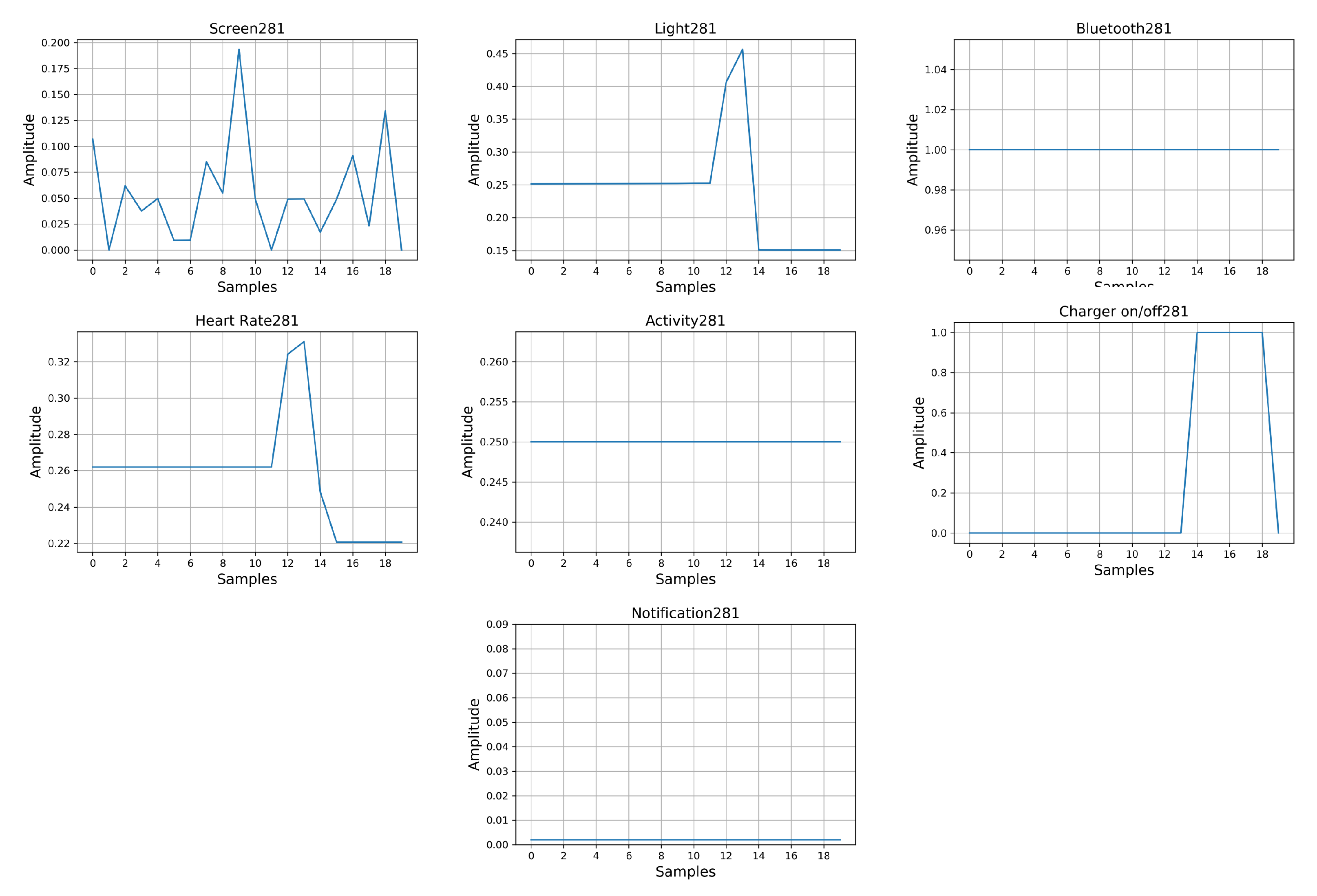
| 281 | 1 | 1 | 99% | 0.62 | 8, 1 |
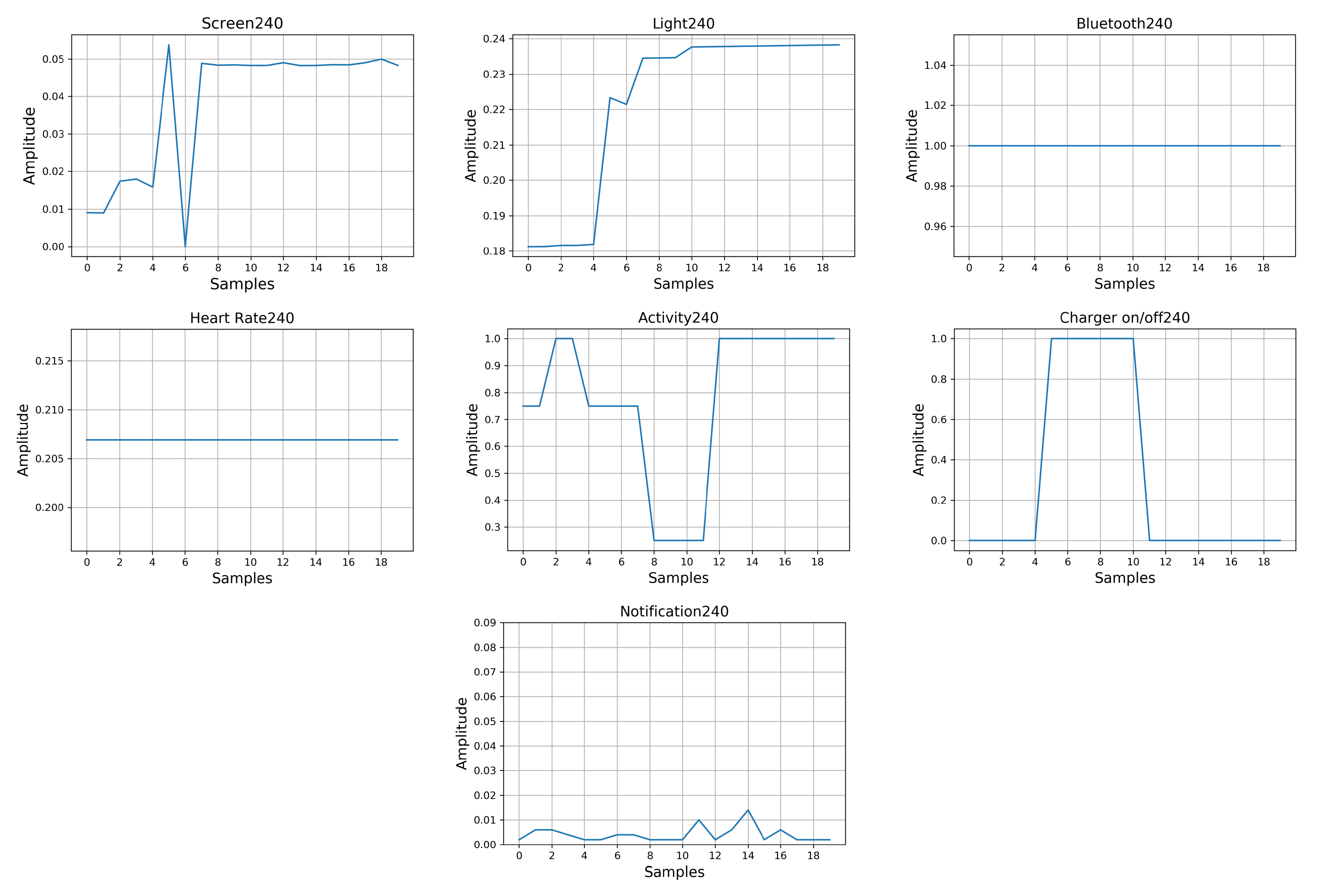
| 240 | 1 | 1 | 99% | 0.66 | 8 |
| 190 | 1 | 1 | 72% | 0.30 | 8 |
| 129 | 0 | 0 | 97% | 0.1 | 8 |
| 92 | 1 | 0 | 95% | 0.71 | 8, 1 |
| 46 | 0 | 1 | 74% | 0.06 | 8 |
| Brands | Average | Wear OS Version | Average |
|---|---|---|---|
| Motorola | 0.004 | 5.1.1 | −0.004 |
| LGE | −0.009 | 6.0.1 | −0.0002 |
| Asus | −0.026 | 7.1.1 | −0.0209 |
| Huawei | −0.033 | - | - |
| Sony | 0.009 | - | - |
| Mobvoi | −0.01 | - | - |
© 2020 by the authors. Licensee MDPI, Basel, Switzerland. This article is an open access article distributed under the terms and conditions of the Creative Commons Attribution (CC BY) license (http://creativecommons.org/licenses/by/4.0/).
Share and Cite
Homayounfar, M.; Malekijoo, A.; Visuri, A.; Dobbins, C.; Peltonen, E.; Pinsky, E.; Teymourian, K.; Rawassizadeh, R. Understanding Smartwatch Battery Utilization in the Wild. Sensors 2020, 20, 3784. https://doi.org/10.3390/s20133784
Homayounfar M, Malekijoo A, Visuri A, Dobbins C, Peltonen E, Pinsky E, Teymourian K, Rawassizadeh R. Understanding Smartwatch Battery Utilization in the Wild. Sensors. 2020; 20(13):3784. https://doi.org/10.3390/s20133784
Chicago/Turabian StyleHomayounfar, Morteza, Amirhossein Malekijoo, Aku Visuri, Chelsea Dobbins, Ella Peltonen, Eugene Pinsky, Kia Teymourian, and Reza Rawassizadeh. 2020. "Understanding Smartwatch Battery Utilization in the Wild" Sensors 20, no. 13: 3784. https://doi.org/10.3390/s20133784
APA StyleHomayounfar, M., Malekijoo, A., Visuri, A., Dobbins, C., Peltonen, E., Pinsky, E., Teymourian, K., & Rawassizadeh, R. (2020). Understanding Smartwatch Battery Utilization in the Wild. Sensors, 20(13), 3784. https://doi.org/10.3390/s20133784