SSD-TSEFFM: New SSD Using Trident Feature and Squeeze and Extraction Feature Fusion


Abstract
1. Introduction
- A novel model with an accuracy higher than that of the SSD is proposed.
- TFM enhances the robustness of the model to feature maps with various scales in the proposed method.
- The proposed model, SSD-TSEFFM, addresses the challenges encountered in the detection of small objects.
2. Related Work
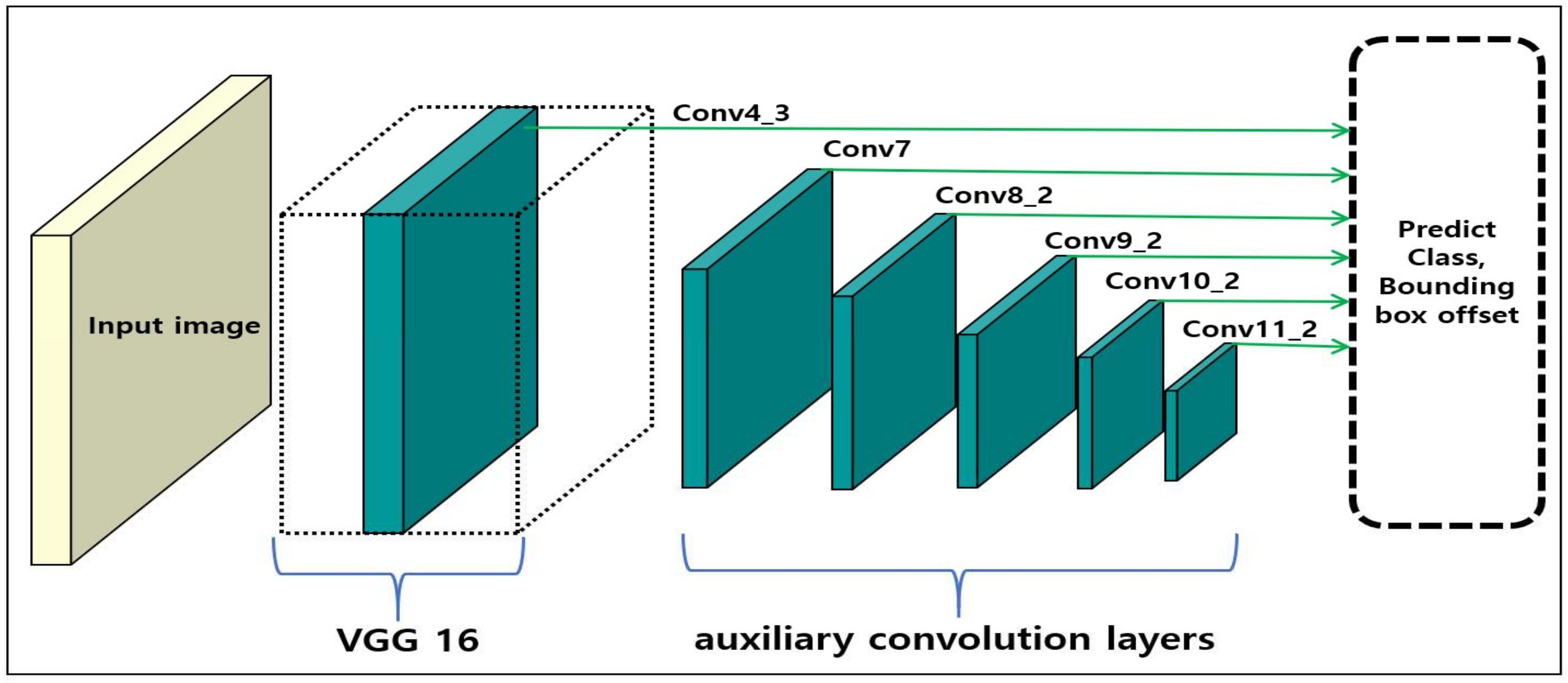
2.1. SSD Series
2.2. Object Detectors for Scale-Variance
2.3. Feature Pyramid Network
2.4. Squeeze and Excitation (SE) Block
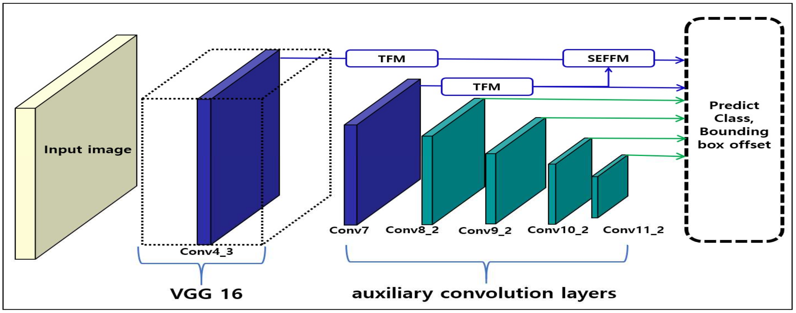
3. Proposed Model
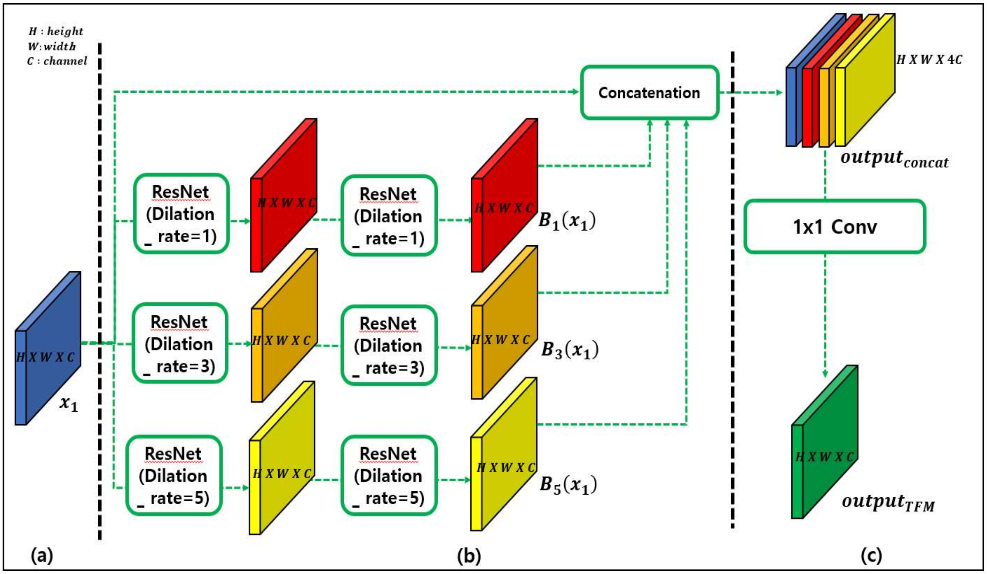
3.1. Trident Feature Module (TFM)
3.2. SE-Feature Fusion Module (SEFFM)
4. Experiment
4.1. Training Setting
4.2. Experiment Results
- ▪
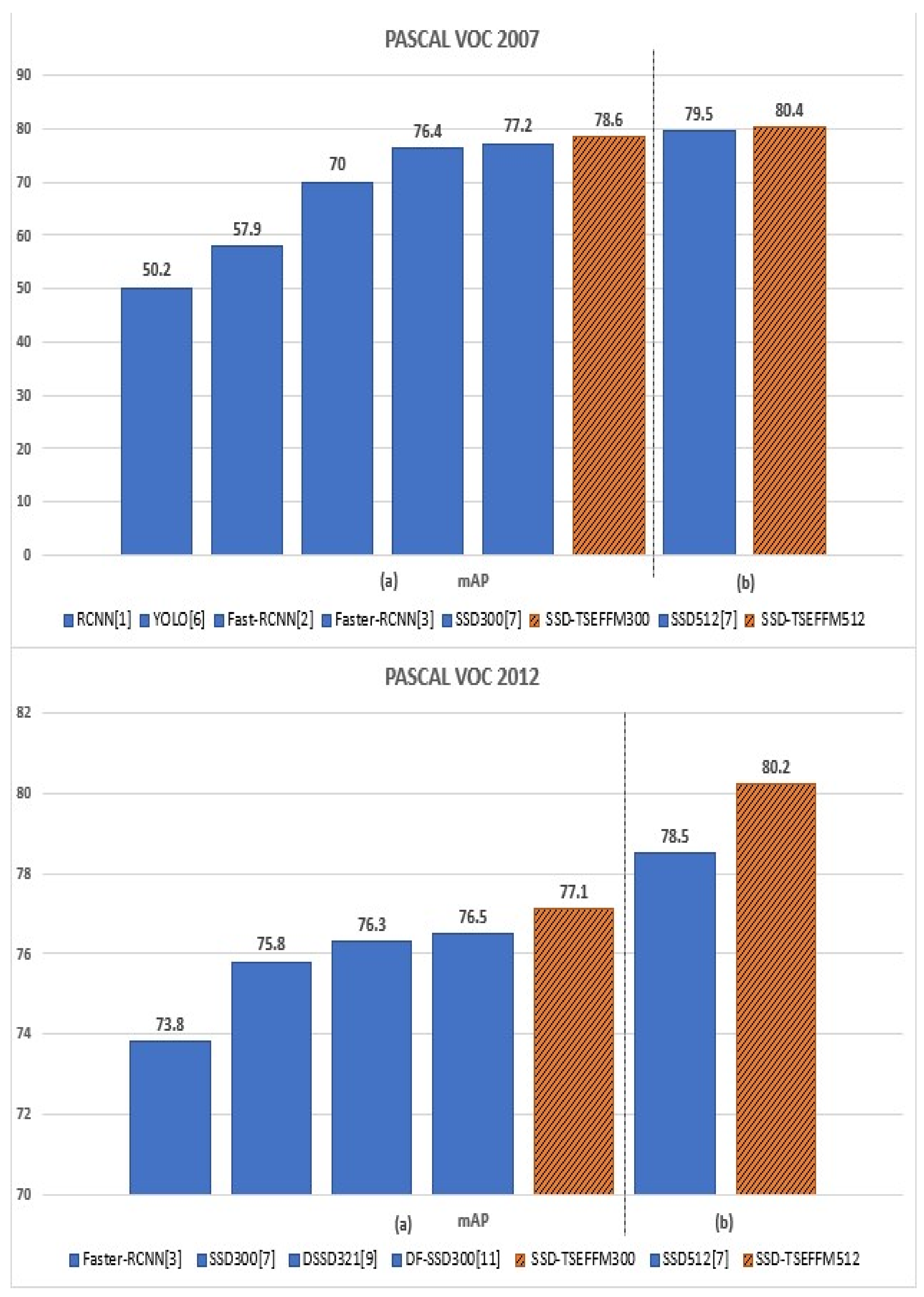
- Results on PASCAL VOC 2007 dataset
- ▪
- Results on PASCAL VOC 2012 dataset
4.3. TFM Application Results
5. Conclusions
Author Contributions
Funding
Conflicts of Interest
References
- Wu, Y.; Tang, S.; Zhang, S.; Ogai, H. An Enhanced Feature Pyramid Object Detection Network for Autonomous Driving. Sensors 2019, 9, 4363. [Google Scholar] [CrossRef]
- Peng, C.; Bu, W.; Xiao, J.; Wong, K.-C.; Yang, M. An Improved Neural Network Cascade for Face Detection in Large Scene Surveillance. Sensors 2018, 8, 2222. [Google Scholar] [CrossRef]
- Zhu, X.; Ding, M.; Huang, T.; Jin, X.; Zhang, X. PCANet-Based Structural Representation for Nonrigid Multimodal Medical Image Registration. Sensors 2018, 18, 1477. [Google Scholar] [CrossRef] [PubMed]
- Calì, M.; Ambu, R. Advanced 3D Photogrammetric Surface Reconstruction of Extensive Objects by UAV Camera Image Acquisition. Sensors 2018, 18, 2815. [Google Scholar] [CrossRef] [PubMed]
- Ryu, J.; Kim, S. Chinese Character Boxes: Single Shot Detector Network for Chinese Character Detection. Sensors 2019, 9, 315. [Google Scholar] [CrossRef]
- Ali, S.; Scovanner, P.; Shah, M. A 3-Dimensional SIFT descriptor and its application to action recognition. In Proceedings of the 15th International Conference on Multimedia, Augsburg, Germany, 24–29 September 2007; pp. 357–360. [Google Scholar]
- Dalal, N.; Triggs, B. Histograms of oriented gradients for human detection. In Proceedings of the IEEE Conference on Computer Vision and Pattern Recognition (CVPR 2005), San Diego, CA, USA, 25 June 2005; Volume 1, pp. 886–893. [Google Scholar]
- Lowe, D. Distinctive image features from scale-invariant keypoints. Int. J. Comput. Vis. 2004, 60, 91–110. [Google Scholar] [CrossRef]
- Finlayson, G.; Hordley, S.; Schaefer, G.; Tian, G.Y. Illuminant and device invariant colour using histogram equalisation. Pattern Recognit. 2005, 38, 179–190. [Google Scholar] [CrossRef]
- Girshick, R.; Donahue, J.; Darrell, T.; Malik, J. Rich feature hierarchies for accurate object detection and semantic segmentation. In Proceedings of the IEEE Conference on Computer Vision and Pattern Recognition (CVPR 2014), Columbus, OH, USA, 23–28 June 2014; pp. 580–587. [Google Scholar]
- Girshick, R. Fast R-CNN. In Proceedings of the International Conference on Computer Vision, Santiago, Chile, 7–13 December 2015; pp. 1440–1448. [Google Scholar]
- Ren, S.; He, K.; Girshick, R.; Sun, J. Faster r-cnn: Towards real-time object detection with region proposal networks. In Advances in Neural Information Processing Systems, Proceedings of the Neural Information Processing Systems Conference (NIPS 2015), Montreal, QC, Canada, 7–12 December 2015; Neural Information Processing Systems Foundation, Inc.: Ljubljana, Slovenia, 2015; pp. 91–99. [Google Scholar]
- He, K.; Gkioxari, G.; Dollar, P.; Girshick, R. Mask R-CNN. In Proceedings of the 16th IEEE International Conference on Computer Vision (ICCV 2017), Venice, Italy, 22–29 October 2017; pp. 2980–2988. [Google Scholar]
- Lin, T.Y.; Dollár, P.; Girshick, R.; He, K.; Hariharan, B.; Belongie, S. Feature pyramid networks for object detection. In Proceedings of the IEEE Conference on Computer Vision and Pattern Recognition (CVPR 2017), Minneapolis, MN, USA, 17–22 June 2017; Volume 1, p. 4. [Google Scholar]
- Redmon, J.; Divvala, S.; Girshick, R.; Farhadi, A. You Only Look Once: Unified, Real-Time Object Detection. In Proceedings of the 2015 IEEE Conference on Computer Vision and Pattern Recognition (CVPR 2015), Boston, MA, USA, 7–12 June 2015; pp. 779–788. [Google Scholar]
- Liu, W.; Anguelov, D.; Erhan, D.; Szegedy, C.; Fu, C.; Berg, A.C. SSD: Single Shot Multibox Detector. In Proceedings of the European Conference on Computer Vision, Amsterdam, The Netherlands, 8–16 October 2016; pp. 21–37. [Google Scholar]
- Lin, T.-Y.; Goyal, P.; Girshick, R.; He, K.; Dollar, P. Focal loss for dense object detection. In Proceedings of the 2017 IEEE International Conference on Computer Vision (ICCV 2017), Venice, Italy, 22–29 October 2017. [Google Scholar]
- Fu, C.Y.; Liu, W.; Ranga, A.; Tyagi, A.; Berg, A.C. DSSD: Deconvolutional single shot detector. In Proceedings of the IEEE Conference on Computer Vision and Pattern Recognition, Hawaii, HI, USA, 21–26 July 2017; pp. 1–8. [Google Scholar]
- Jeong, J.; Park, H.; Kwak, N. Enhancement of SSD by concatenating feature maps for object detection. In Proceedings of the British Machine Vision Conference (BMVC 2017), London, UK, 4–7 September 2017. [Google Scholar]
- Zhai, S.; Shang, D.; Wang, S.; Dong, S. DF-SSD: An Improved SSD Object Detection Algorithm Based on Dense Net and Feature Fusion. IEEE Access 2020, 8, 24344–24357. [Google Scholar] [CrossRef]
- Li, Y.; Chen, Y.; Wang, N.; Zhang, Z. Scale-Aware Trident Networks for Object Detection. In Proceedings of the IEEE International Conference on Computer Vision (ICCV 2019), Seoul, Korea, 27 October–2 November 2019; pp. 6054–6063. [Google Scholar]
- Yu, J.; Shen, L.; Sun, G. Squeeze-and-Excitation Networks. In Proceedings of the IEEE Conference on Computer Vision and Pattern Recognition (CVPR 2018), Salt Lake City, UT, USA, 18–22 June 2018. [Google Scholar]
- Everingham, M.; Van Gool, L.; Williams, C.K.; Winn, J.; Zisserman, A. The PASCAL visual object classes (voc) challenge. Int. J. Comput. Vis. 2010, 88, 303–338. [Google Scholar] [CrossRef]
- Simonyan, K.; Zisserman, A. Very deep convolutional networks for large-scale image recognition. arXiv 2014, arXiv:1409.1556. [Google Scholar]
- Singh, B.; Davis, L.S. An Analysis of Scale Invariance in Object Detection—SNIP. In Proceedings of the 2018 IEEE/CVF Conference on Computer Vision and Pattern Recognition, Salt Lake City, UT, USA, 19–21 June 2018; Institute of Electrical and Electronics Engineers (IEEE): Piscataway, NJ, USA, 2018; pp. 3578–3587. [Google Scholar]
- Adelson, E.H.; Anderson, C.H.; Bergen, J.R.; Burt, P.J.; Ogden, M.J. Pyramid methods in image processing. RCA Eng. 1984, 29, 33–41. [Google Scholar]
- Singh, B.; Najibi, M.; Davis, L.S. SNIPER: Efficient Multi-Scale Training. In Proceedings of the Advances in Neural Information Processing Systems (NIPS 2018), Montreal, QC, Canada, 2–8 December 2018. [Google Scholar]
- Yu, F.; Koltun, V. Multi-scale context aggregation by dilated convolutions. In Proceedings of the 2016 International Conference on Learning Representations, San Juan, Puerto Rico, 2–4 May 2016. [Google Scholar]
- He, K.; Zhang, X.; Ren, S.; Sun, J. Deep Residual Learning for Image Recognition. In Proceedings of the European Conference on Computer Vision, Amsterdam, The Netherlands, 8–16 October 2016; pp. 770–778. [Google Scholar]
- Russakovsky, O.; Deng, J.; Su, H.; Krause, J.; Satheesh, S.; Ma, S.; Huang, Z.; Karpathy, A.; Khosla, A.; Bernstein, M. ImageNet Large Scale Visual Recognition Challenge. Int. J. Comput. Vis. 2014, 115, 211–252. [Google Scholar] [CrossRef]
- Glorot, X.; Bengio, Y. Understanding the difficulty of training deep feedforward neural networks. In Proceedings of the Thirteenth International Conference on Artificial Intelligence and Statistics, Sardinia, Italy, 13–15 May 2010; pp. 249–256. [Google Scholar]
- Paszke, A.; Gross, S.; Chintala, S.; Chanan, G.; Yang, E.; DeVito, Z.; Lin, Z.; Desmaison, A.; Antiga, L.; Lerer, A. Automatic differentiation in PyTorch. In Proceedings of the Advances in Neural Information Processing Systems (NIPS) Workshops, Long Beach, CA, USA, 8–9 December 2017. [Google Scholar]
- Chetlur, S.; Woolley, C.; Vandermersch, P.; Cohen, J.; Tran, J.; Catanzaro, B.; Shelhamer, E. cudnn: Efficient primitives for deep learning. arXiv 2014, arXiv:1410.0759. [Google Scholar]


| Network | mAP | Aero | Bike | Bird | Boat | Bottle | Bus | Car | Cat | Chair | Cow | Table | Dog | Horse | Mbike | Persn | Plant | Sheep | Sofa | Train | tv |
|---|---|---|---|---|---|---|---|---|---|---|---|---|---|---|---|---|---|---|---|---|---|
| 300 × 300 input | |||||||||||||||||||||
| RCNN [5] | 50.2 | 67.1 | 64.1 | 46.7 | 32.0 | 30.5 | 56.4 | 57.2 | 65.9 | 27.0 | 47.3 | 40.9 | 66.6 | 57.8 | 65.9 | 53.6 | 26.7 | 56.5 | 38.1 | 52.8 | 50.2 |
| Fast-RCNN [11] | 70.0 | 77.0 | 78.1 | 69.3 | 59.4 | 38.3 | 81.6 | 78.6 | 86.7 | 42.8 | 78.8 | 68.9 | 84.7 | 82.0 | 76.6 | 69.9 | 31.8 | 70.1 | 74.8 | 80.4 | 70.4 |
| Faster-RCNN [12] | 76.4 | 79.8 | 80.7 | 76.2 | 68.3 | 55.9 | 85.1 | 85.3 | 89.8 | 56.7 | 87.8 | 69.4 | 88.3 | 88.9 | 80.9 | 78.4 | 41.7 | 78.6 | 79.8 | 85.3 | 72.0 |
| YOLO [15] | 57.9 | 77.0 | 67.2 | 57.7 | 38.3 | 22.7 | 68.3 | 55.9 | 81.4 | 36.2 | 60.8 | 48.5 | 77.2 | 72.3 | 71.3 | 63.5 | 28.9 | 52.2 | 54.8 | 73.9 | 50.8 |
| SSD300 [16] | 77.2 | 78.8 | 85.3 | 75.7 | 71.5 | 49.1 | 85.7 | 86.4 | 87.8 | 60.6 | 82.7 | 76.5 | 84.9 | 86.7 | 84.0 | 79.2 | 51.3 | 77.5 | 78.7 | 86.7 | 76.2 |
| SSD-TSEFFM300 | 78.6 | 81.6 | 94.6 | 79.1 | 72.1 | 50.2 | 86.4 | 86.9 | 89.1 | 60.3 | 85.6 | 75.7 | 85.6 | 88.3. | 84.1 | 79.6 | 54.6 | 82.1 | 80.2 | 87.1 | 79.0 |
| 512 × 512 input | |||||||||||||||||||||
| SSD512 | 79.5 | 84.8 | 85.1 | 81.5 | 73.0 | 57.8 | 87.8 | 88.3 | 87.4 | 63.5 | 85.4 | 73.2 | 86.2 | 86.7 | 83.9 | 82.5 | 55.6 | 81.7 | 79.0 | 86.6 | 80.0 |
| SSD-TSEFFM512 | 80.4 | 84.9 | 86.7 | 80.6 | 76.2 | 59.4 | 87.8 | 88.9 | 89.2 | 61.7 | 86.9 | 78.3 | 86.2 | 88.8 | 85.6 | 82.7 | 55.4 | 82.7 | 79.4 | 84.7 | 81.3 |
| Network | mAP | Aero | Bike | Bird | Boat | Bottle | Bus | Car | Cat | Chair | Cow | Table | Dog | Horse | Mbike | Persn | Plant | Sheep | Sofa | Train | tv |
|---|---|---|---|---|---|---|---|---|---|---|---|---|---|---|---|---|---|---|---|---|---|
| 300 × 300 input | |||||||||||||||||||||
| Faster-RCNN [12] | 73.8 | 86.5 | 81.6 | 77.2 | 58.0 | 51.0 | 78.6 | 76.6 | 93.2 | 48.6 | 80.4 | 59.0 | 92.1 | 85.3 | 84.8 | 80.7 | 48.1 | 77.3 | 66.5 | 84.7 | 65.6 |
| SSD300 [16] | 75.8 | 88.1 | 82.9 | 74.4 | 61.9 | 47.6 | 82.7 | 78.8 | 91.5 | 58.1 | 80.0 | 64.1 | 89.4 | 85.7 | 85.5 | 82.6 | 50.2 | 79.8 | 73.6 | 86.6 | 72.1 |
| DSSD321 [18] | 76.3 | 87.3 | 83.3 | 75.4 | 64.6 | 46.8 | 82.7 | 76.5 | 92.9 | 59.5 | 78.3 | 64.3 | 91.5 | 86.6 | 86.6 | 82.1 | 53.3 | 79.6 | 75.7 | 85.2 | 73.9 |
| DF-SSD300 [20] | 76.5 | 89.5 | 85.6 | 72.6 | 65.8 | 51.3 | 82.9 | 79.9 | 92.2 | 62.4 | 77.5 | 64.5 | 89.5 | 85.4 | 86.4 | 85.7 | 51.9 | 77.8 | 72.6 | 85.1 | 71.6 |
| SSD-TSEFFM300 | 77.1 | 88.6 | 85.9 | 76.0 | 65.4 | 46.2 | 84.0 | 79.9 | 92.7 | 58.6 | 81.9 | 65.3 | 91.5 | 87.8 | 88.8 | 82.9 | 52.6 | 79.1 | 75.4 | 87.1 | 73.8 |
| 512 × 512 input | |||||||||||||||||||||
| SSD512 | 78.5 | 90.0 | 85.3 | 77.7 | 64.3 | 58.5 | 85.1 | 84.3 | 92.6 | 61.3 | 83.4 | 65.1 | 89.9 | 88.5 | 88.2 | 85.5 | 54.4 | 82.4 | 70.7 | 87.1 | 75.6 |
| SSD-TSEFFM512 | 80.2 | 90.1 | 88.2 | 81.5 | 68.4 | 59.1 | 85.6 | 85.5 | 93.7 | 63.0 | 86.1 | 64.0 | 90.9 | 88.6 | 89.1 | 86.4 | 59.2 | 85.9 | 73.3 | 87.8 | 75.9 |
| Network | mAP | Conv4_3 | Conv7 | Conv8_2 | Conv9_2 | Conv10_2 | Conv11_2 |
|---|---|---|---|---|---|---|---|
| Original SSD | 77.2 | ||||||
| SSD-TSEFFM | 77.5 | V | |||||
| SSD-TSEFFM | 78.6 | V | V | ||||
| SSD-TSEFFM | 78.7 | V | V | V | |||
| SSD-TSEFFM | 78.7 | V | V | V | V | ||
| SSD-TSEFFM | 77.7 | V | V | V | V | V | |
| SSD-TSEFFM | 77.8 | V | V | V | V | V | V |
© 2020 by the authors. Licensee MDPI, Basel, Switzerland. This article is an open access article distributed under the terms and conditions of the Creative Commons Attribution (CC BY) license (http://creativecommons.org/licenses/by/4.0/).
Share and Cite
Hwang, Y.-J.; Lee, J.-G.; Moon, U.-C.; Park, H.-H. SSD-TSEFFM: New SSD Using Trident Feature and Squeeze and Extraction Feature Fusion. Sensors 2020, 20, 3630. https://doi.org/10.3390/s20133630
Hwang Y-J, Lee J-G, Moon U-C, Park H-H. SSD-TSEFFM: New SSD Using Trident Feature and Squeeze and Extraction Feature Fusion. Sensors. 2020; 20(13):3630. https://doi.org/10.3390/s20133630
Chicago/Turabian StyleHwang, Young-Joon, Jin-Gu Lee, Un-Chul Moon, and Ho-Hyun Park. 2020. "SSD-TSEFFM: New SSD Using Trident Feature and Squeeze and Extraction Feature Fusion" Sensors 20, no. 13: 3630. https://doi.org/10.3390/s20133630
APA StyleHwang, Y.-J., Lee, J.-G., Moon, U.-C., & Park, H.-H. (2020). SSD-TSEFFM: New SSD Using Trident Feature and Squeeze and Extraction Feature Fusion. Sensors, 20(13), 3630. https://doi.org/10.3390/s20133630