Real-Time Detection on SPAD Value of Potato Plant Using an In-Field Spectral Imaging Sensor System


Abstract
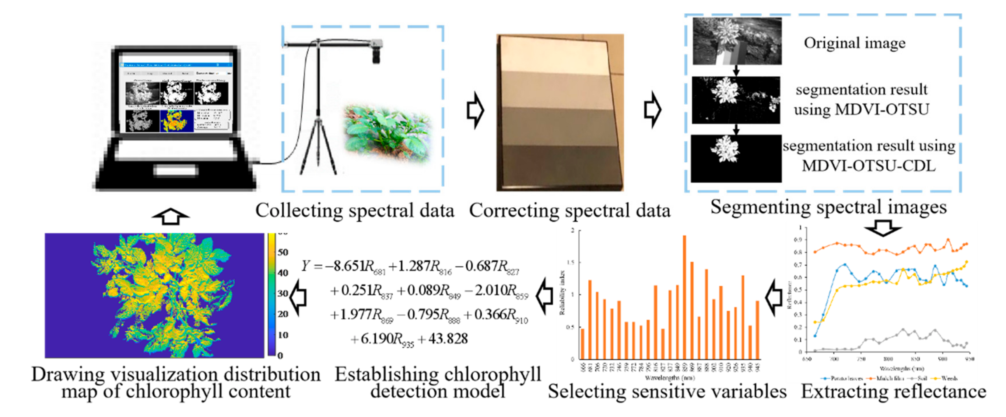
1. Introduction
- (1)
- Automatically segment potato plants using the MDVI–OTSU method,
- (2)
- Automatically extract the reflectance of potato plants using segmented mask images,
- (3)
- Detect the SPAD value of potato plants in real time using the established model,
- (4)
- Generate a visualization distribution map of SPAD value of potato plant based on the spectral images and PLS model.
2. Materials and Methods
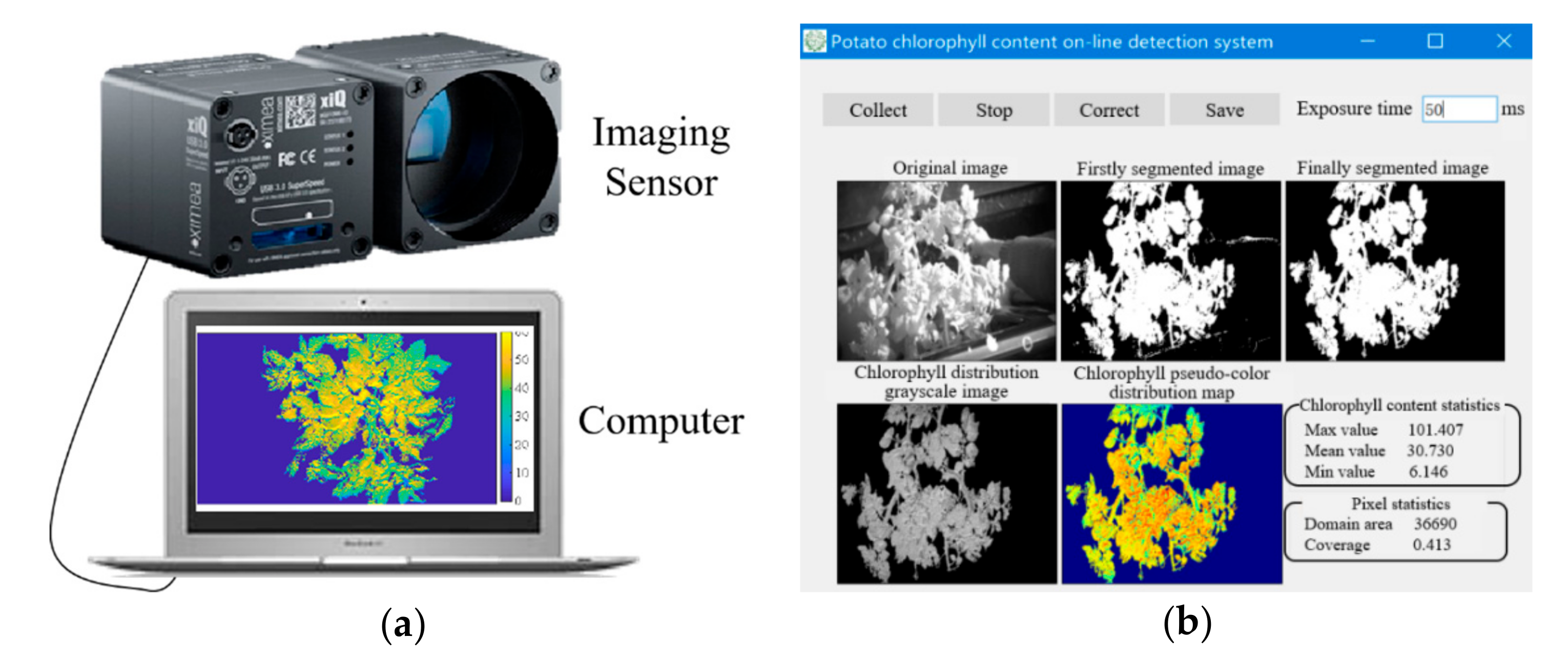
2.1. Development of SPAD Value Detection System
2.2. Data Acquisition
2.2.1. Spectral Image Collection of Potato Plants
2.2.2. SPAD Value Measurement
2.2.3. Reflectance Correction of Spectral Images
2.3. Segmentation Method of Spectral Images
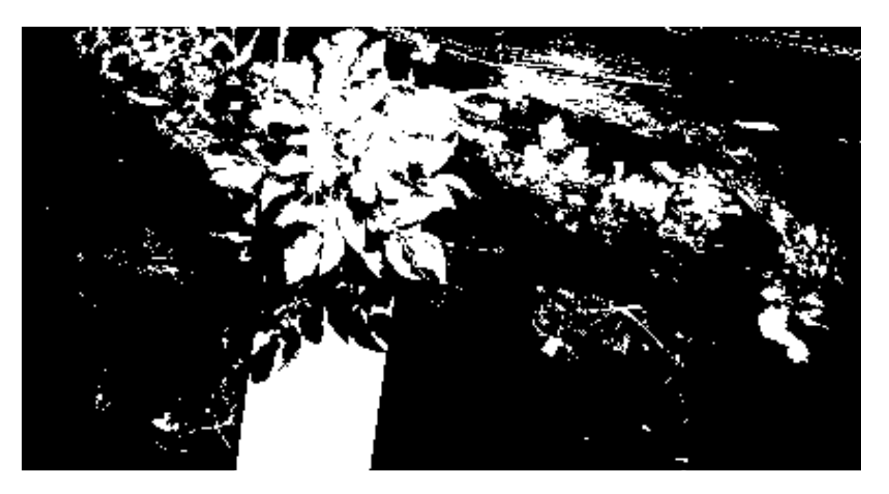
2.3.1. MDVI–OTSU Method (Preliminary Segmentation)
2.3.2. Connected Domain-Labeling Method (Precision Segmentation)
2.3.3. Evaluation of Image Segmentation Accuracy
2.4. Establishment of the Detection Model
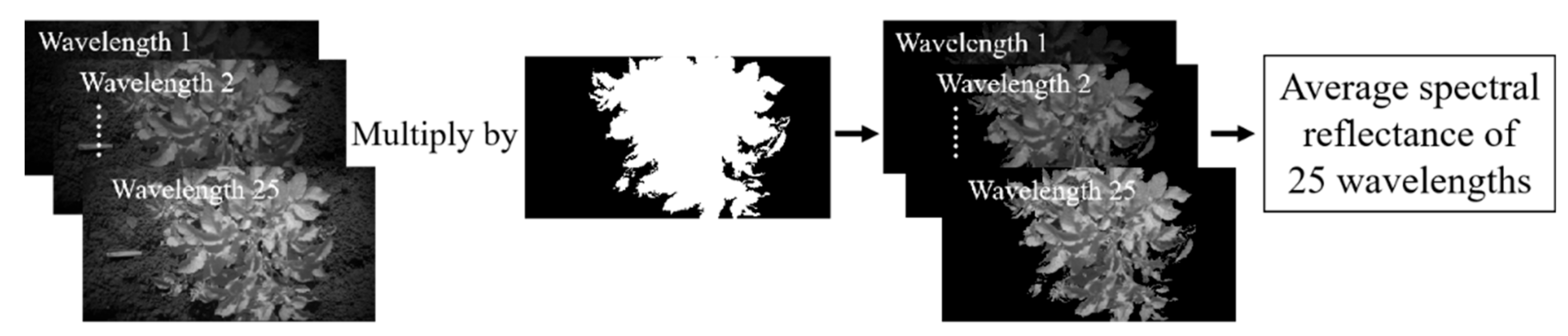
2.4.1. Reflectance Spectra Calculation
2.4.2. Uninformative Variable Elimination
2.4.3. Partial Least Squares Regression
2.4.4. Application of the Dataset
2.5. Visualization Distribution Map of Potato SPAD Value
- (1)
- Extract spectral images of potato leaves at characteristic wavelengths,
- (2)
- Extract the reflectance of each pixel in the corresponding characteristic wavelength images,
- (3)
- Calculate the SPAD value of each pixel by using the PLSR model to form a grayscale image,
- (4)
- Draw the Visualization distribution map of SPAD value of potato by performing pseudo-color processing on the grayscale image.
3. Results and Discussion
3.1. Spectral Image Segmentation Results
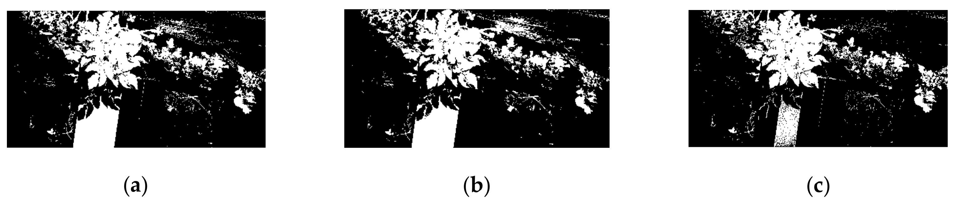
3.1.1. Preliminary Segmentation Results Using the MDVI–OTSU Method
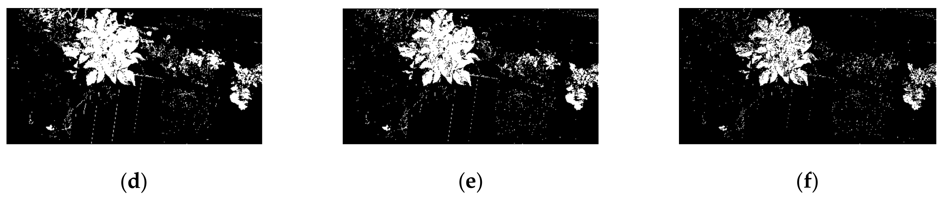
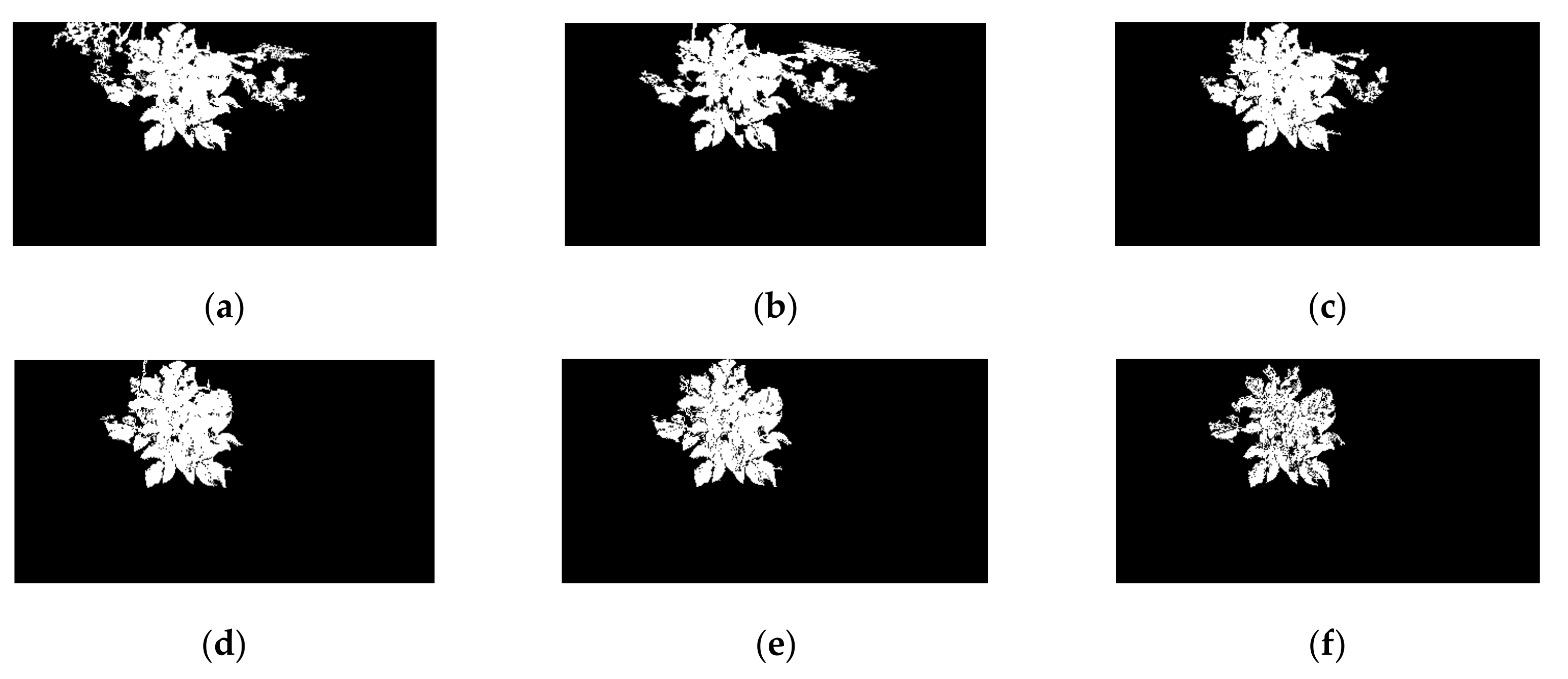
3.1.2. Precision Segmentation Results Using the MDVI–OTSU–CDL Method
3.1.3. Comparison of Segmentation Accuracy
3.2. Data Characteristics Analysis
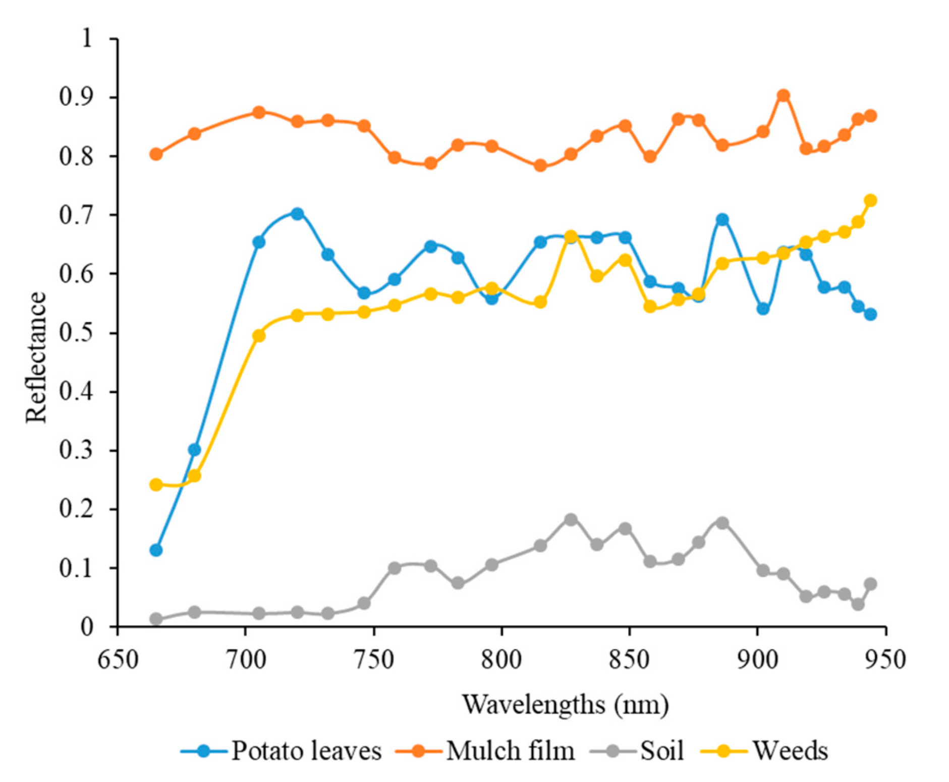
3.2.1. Spectral Response of Potato Plant at 25 Wavelengths
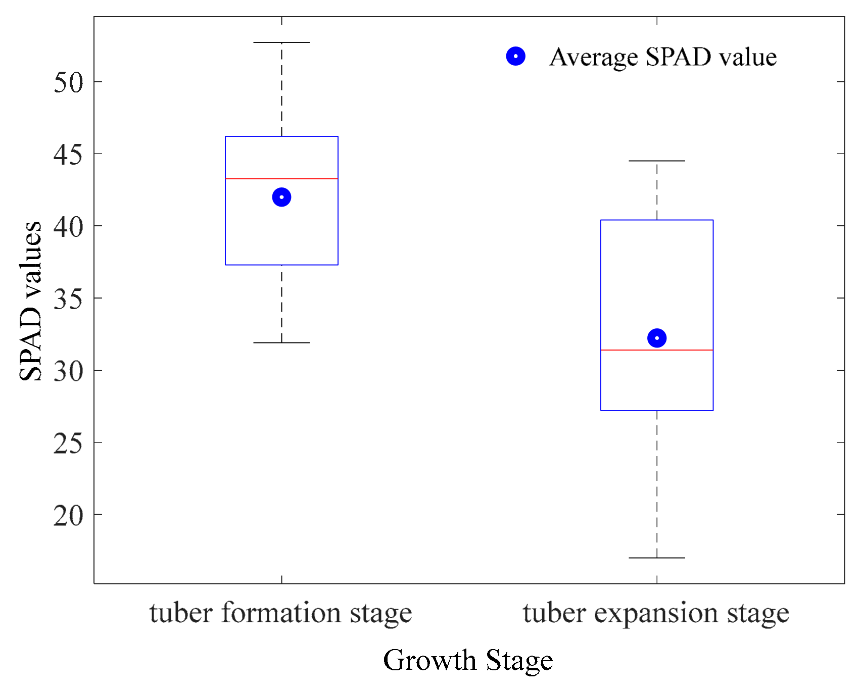
3.2.2. SPAD Value Statistics of Modeling Dataset
3.3. Detection of SPAD Value of Potato Plants
3.3.1. Influence of Modified Coefficients on PLS Model
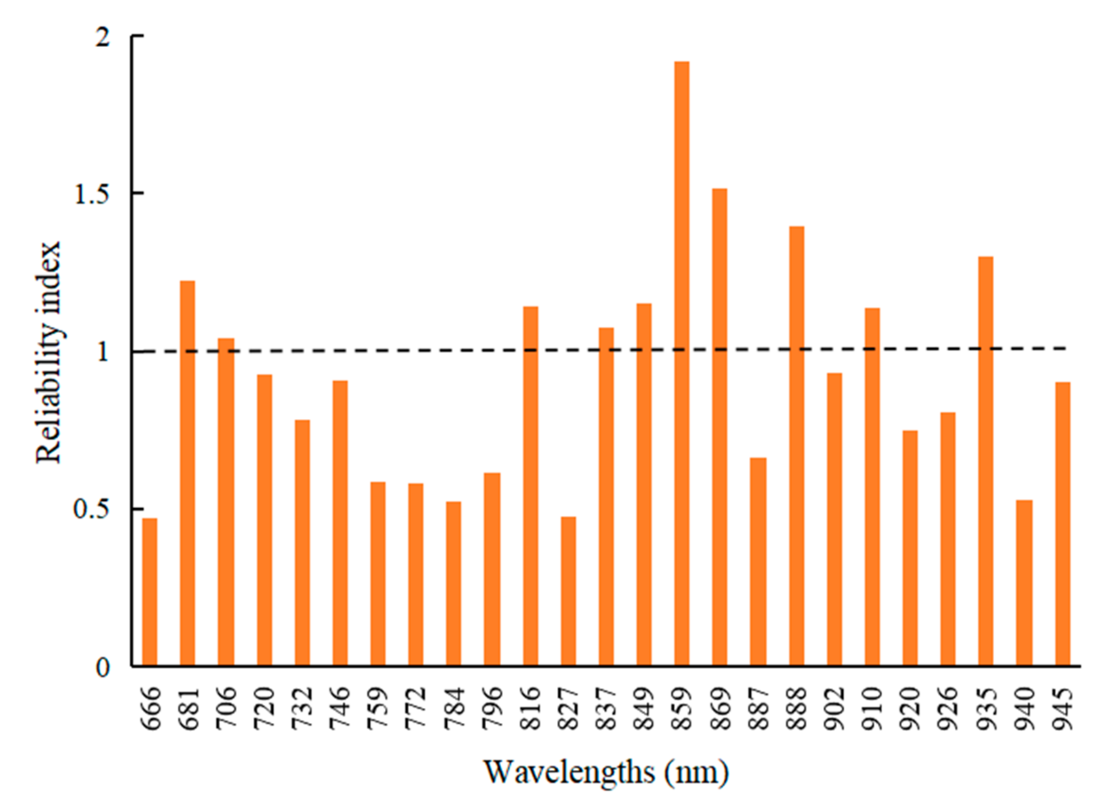
3.3.2. Sensitive Variables Selection
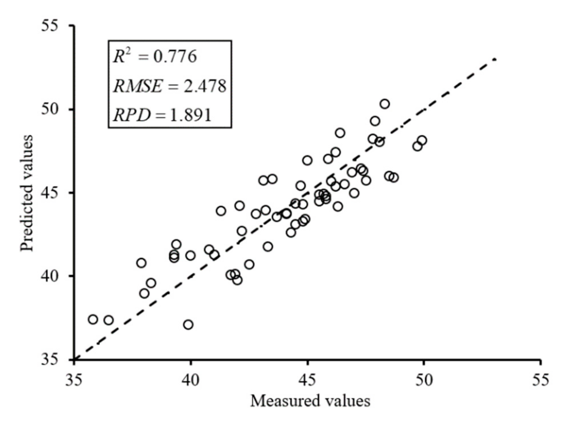
3.3.3. Establishment of UVE–PLS Model
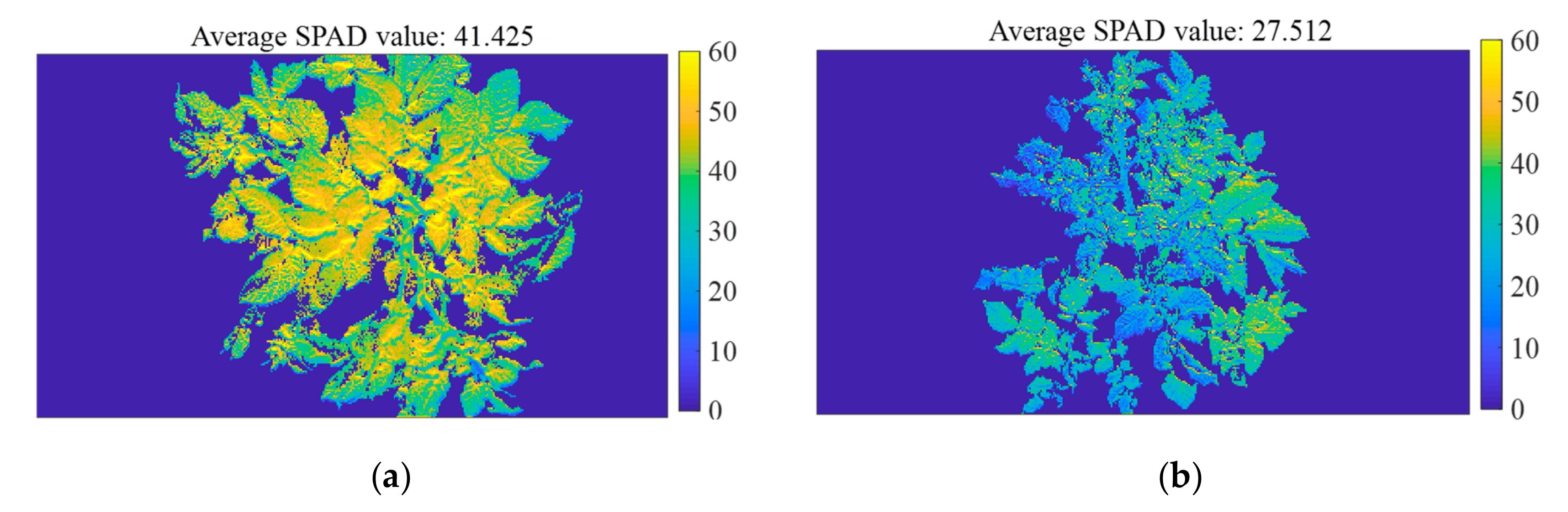
3.4. Visualization Distribution Map of SPAD Value
3.5. Testing of the Developed Detection System
4. Conclusions
Author Contributions
Funding
Acknowledgments
Conflicts of Interest
References
- Hong, Z.; Fen, X.; Yu, W.; Hong-hai, H.; Xiao-feng, D. Progress of potato staple food research and industry development in China. J. Integr. Agric. 2017, 16, 2924–2932. [Google Scholar] [CrossRef]
- Alva, A.; Fan, M.; Chen, Q.; Rosen, C.; Ren, H. Improving Nutrient-Use Efficiency in Chinese Potato Production: Experiences from the United States. J. Crop Improv. 2011, 25, 46–85. [Google Scholar] [CrossRef]
- Vesali, F.; Omid, M.; Mobli, H.A. Kaleita. Feasibility of using smart phones to estimate chlorophyll content in corn plants. Photosynthetica 2017, 55, 603–610. [Google Scholar] [CrossRef]
- Gaurav, S.; Babankumar, B.; Lini, M.; Jonali, G.; Burhan, U.C.; Raju, P.L.N. Chlorophyll estimation using multi-spectral unmanned aerial system based on machine learning techniques. Remote Sens. Appl.: Soc. Environ. 2019, 15, 100235. [Google Scholar] [CrossRef]
- Zhou, Z.; Jabloun, M.; Plauborg, F.; Andersen, M.N. Using ground-based spectral reflectance sensors and photography to estimate shoot N concentration and dry matter of potato. Comput. Electron. Agric. 2018, 144, 154–163. [Google Scholar] [CrossRef]
- Clevers, J.G.P.W.; Kooistra, L. Using Hyperspectral Remote Sensing Data for Retrieving Canopy Chlorophyll and Nitrogen Content. IEEE J. Sel. Top. Appl. Earth Obs. Remote Sens. 2012, 5, 574–583. [Google Scholar] [CrossRef]
- Nigon, T.J.; Mulla, D.J.; Rosen, C.J.; Cohen, Y.; Alchanatis, V.; Rud, R. Evaluation of the nitrogen sufficiency index for use with high resolution, broadband aerial imagery in a commercial potato field. Precis. Agric. 2014, 15, 202–226. [Google Scholar] [CrossRef]
- Ali, M.M.; Al-Ani, A.; Eamus, D.; Tan, D.K. A new image processing-based technique to determine chlorophyll in plants. Am.-Eurasian J. Agricult. Environ. Sci. 2012, 12, 1323–1328. [Google Scholar] [CrossRef]
- Kira, O.; Linker, R.; Gitelson, A. Non-destructive estimation of foliar chlorophyll and carotenoid contents: Focus on informative spectral bands. International J. Appl. Earth Obs. Geoinf. 2015, 38, 251–260. [Google Scholar] [CrossRef]
- He, C.; Zheng, S.; Wan, N.; Zhao, T.; Yuan, J.; He, W.; Hu, J. Potato spectrum and the digital image feature parameters on the response of the nitrogen level and its application. Spectrosc. Spectr. Anal. 2016, 36, 2930–2936. [Google Scholar] [CrossRef]
- Yuan, Z.; Cao, Q.; Zhang, K.; Ata-Ul-Karim, S.T.; Tian, Y.; Zhu, Y.; Cao, W.; Liu, X. Optimal Leaf Positions for SPAD Meter Measurement in Rice. Front. Plant Sci. 2016, 7. [Google Scholar] [CrossRef] [PubMed]
- Adamsen, F.J.; Pinter, P.J.; Barnes, E.M.; LaMorte, R.L.; Wall, G.W.; Leavitt, S.; Kimball, B.A. Measuring wheat senescence with a digital camera. Crop Sci. 1999, 719–724. [Google Scholar] [CrossRef]
- Uddling, J.; Gelang-Alfredsson, J.; Piikki, K.; Pleijel, H. Evaluating the relationship between leaf chlorophyll concentration and SPAD-502 chlorophyll meter readings. Photosynth. Res. 2007, 91, 37–46. [Google Scholar] [CrossRef]
- Monje, O.A.; Bugbee, B. Inherent Limitations of Nondestructive Chlorophyll Meters: A Comparison of Two Types of Meters. HortScience 1992, 27, 69–71. [Google Scholar] [CrossRef] [PubMed]
- Ling, Q.; Huang, W.; Jarvis, P. Use of a SPAD-502 meter to measure leaf chlorophyll concentration in Arabidopsis thaliana. Photosynth. Res. 2011, 107, 209–214. [Google Scholar] [CrossRef]
- Vos, J.; Bom, M. Hand-held chlorophyll meter: A promising tool to assess the nitrogen status of potato foliage. Potato Res. 1993, 36, 301–308. [Google Scholar] [CrossRef]
- Dvořák, P. Response of Surface Mulching of Potato (Solanum tuberosum) on SPAD Value, Colorado Potato Beetle and Tuber Yield. Int. J. Agric. Biol. 2013, 15, 798–800. [Google Scholar] [CrossRef][Green Version]
- Wang, H.; Huo, Z.; Zhou, G.; Liao, Q.; Feng, H.; Wu, L. Estimating leaf SPAD values of freeze-damaged winter wheat using continuous wavelet analysis. Plant Physiol. Biochem. 2016, 98, 39–45. [Google Scholar] [CrossRef]
- Sun, H.; Zheng, T.; Liu, N.; Cheng, M.; Li, M.; Zhang, Q. Vertical distribution of chlorophyll in potato plants based on hyperspectral imaging. Trans. Chin. Soc. Agric. Eng. 2018, 34, 149–156. [Google Scholar] [CrossRef]
- Qian, W.; Hong, S.; Min-zan, L. Research on Maize Multispectral Image Accurate Segmentation and Chlorophyll Index Estimation. Spectrosc. Spectr. Anal. 2015, 35, 178–183. [Google Scholar] [CrossRef]
- Borhan, M.S.; Panigrahi, S. Evaluation of computer imaging technique for predicting the SPAD readings in potato leaves. Inf. Process. Agric. 2017, 4, 275–282. [Google Scholar] [CrossRef]
- Ranjeeta, A.; Cheng, L.; Kirby, K.; Krishna, N. A low-cost smartphone controlled sensor based on image analysis for estimating whole-plant tissue nitrogen (N) content in floriculture crops. Comput. Electron. Agric. 2020, 169, 105173. [Google Scholar] [CrossRef]
- Wu, C.; Niu, Z.; Tang, Q.; Huang, W. Remote estimation of gross primary production in wheat using chlorophyll-related vegetation indices. Agric. For. Meteorol. 2009, 149, 1015–1021. [Google Scholar] [CrossRef]
- Tao, Z.; Ning, L.; Li, W.; Li, M.; Sun, H.; Zhang, Q.; Wu, J. Estimation of Chlorophyll Content in Potato Leaves Based on Spectral Red Edge Position. IFAC Pap. 2018, 51, 602–606. [Google Scholar] [CrossRef]
- Jeon, H.Y.; Tian, L.F.; Zhu, H. Robust Crop and Weed Segmentation under Uncontrolled Outdoor Illumination. Sensors 2011, 11, 6270–6283. [Google Scholar] [CrossRef]
- Otsu, N. A Threshold Selection Method from Gray-Level Histograms. IEEE Trans. Syst. Man Cybern. 2007, 9, 62–66. [Google Scholar] [CrossRef]
- Esmael, H.; Martin, G.; Edward, J. A survey of image processing techniques for plant extraction and segmentation in the field. Comput. Electron. Agric. 2016, 125, 184–199. [Google Scholar] [CrossRef]
- Meyer, G.E.; Camargo-Neto, J.; Jones, D.D.; Hindman, T.W. Intensified fuzzy clusters for classifying plant, soil, and residue regions of interest from color images. Comput. Electron. Agric. 2004, 42, 161–180. [Google Scholar] [CrossRef]
- Meyer, G.E.; Camargo-Neto, J. Verification of color vegetation indices for automated crop imaging applications. Comput. Electron. Agric. 2008, 63, 282–293. [Google Scholar] [CrossRef]
- Hague, T.; Tillett, N.D.; Wheeler, H. Automated Crop and Weed Monitoring in Widely Spaced Cereals. Precis. Agric. 2006, 7, 21–32. [Google Scholar] [CrossRef]
- Guijarro, M.; Pajares, G.; Riomoros, I.; Herrera, P.J.; Burgos-Artizzu, X.P.; Ribeiro, A. Automatic segmentation of relevant textures in agricultural images. Comput. Electron. Agric. 2011, 75, 75–83. [Google Scholar] [CrossRef]
- Yu, Z.; Cao, Z.; Wu, X.; Bai, X.D.; Qin, Y.; Zhuo, W.; Xiao, Y.; Zhang, X.; Xue, H. Automatic image-based detection technology for two critical growth stages of maize: Emergence and three-leaf stage. Agric. For. Meteorol. 2013, 174, 65–84. [Google Scholar] [CrossRef]
- Guo, W.; Rage, U.K.; Ninomiya, S. Illumination invariant segmentation of vegetation for time series wheat images based on decision tree model. Comput. Electron. Agric. 2013, 96, 58–66. [Google Scholar] [CrossRef]
- Guerrero, J.M.; Pajares, G.; Montalvo, M.; Romeo, J.; Guijarro, M. Support Vector Machines for crop/weeds identification in maize fields. Expert Syst. Appl. 2012, 39, 11149–11155. [Google Scholar] [CrossRef]
- Zheng, L.; Zhang, J.; Wang, Q.Y. Mean-shift-based color segmentation of images containing green vegetation. Comput. Electron. Agric. 2009, 65, 93–98. [Google Scholar] [CrossRef]
- Zheng, L.; Shi, D.; Zhang, J. Segmentation of green vegetation of crop canopy images based on mean shift and Fisher linear discriminant. Pattern Recognit. Lett. 2010, 31, 920–925. [Google Scholar] [CrossRef]
- Dijkstra, T.K.; Henseler, J. Consistent and asymptotically normal PLS estimators for linear structural equations. Comput. Stat. Data Anal. 2015, 81, 10–23. [Google Scholar] [CrossRef]
- Li, H.D.; Xu, Q.S.; Liang, Y.Z. libPLS: An integrated library for partial least squares regression and linear discriminant analysis. Chemom. Intell. Lab. Syst. 2018, 176, 34–43. [Google Scholar] [CrossRef]
- Andries, J.P.M.; Vander, H.Y.; Buydens, L.M.C. Improved variable reduction in partial least squares modelling by Global-Minimum Error Uninformative-Variable Elimination. Anal. Chim. Acta 2017, 982, 37–47. [Google Scholar] [CrossRef]
- Centner, V.; Massart, D.L.; De-Noord, O.; De-Jong, S.; Vandeginste, B.G.M.; Sterna, C. Elimination of Uninformative Variables for Multivariate Calibration. Anal. Chem. 1996, 68, 3851–3858. [Google Scholar] [CrossRef]
- Yao-wei, L.; Hong, S.; De-hua, G.; Zhi-yong, Z.; Min-zan, L.; Wei, Y. Detection of Crop Chlorophyll Content Based on Spectrum Extraction from Coating Imaging Sensor. Spectrosc. Spectr. Anal. 2020, 40, 1581–1587. [Google Scholar] [CrossRef]
- Geladi, P.; Kowalski, B.R. Partial Least-Squares Regression: A Tutorial. Anal. Chim. Acta 1986, 185, 1–17. [Google Scholar] [CrossRef]
- Wang, Z.; Sakuno, Y.; Koike, K.; Ohara, S. Evaluation of Chlorophyll-a Estimation Approaches Using Iterative Stepwise Elimination Partial Least Squares (ISE-PLS) Regression and Several Traditional Algorithms from Field Hyperspectral Measurements in the Seto Inland Sea, Japan. Sensors 2018, 18. [Google Scholar] [CrossRef] [PubMed]
- Han, T.; Linna, Z.; Ming, L.; Yue, W.; Dinggao, S.; Jun, L.; Chengmin, W. Weighted SPXY method for calibration set selection for composition analysis based on near-infrared spectroscopy. Infrared Phys. Technol. 2018, 95, 88–92. [Google Scholar] [CrossRef]


| Wavelength (nm) | FWHM (nm) |
|---|---|
| 666, 681, 706, 720, 732, 746, 759 | 3.35 |
| 772, 784, 796, 816, 827 | 4.69 |
| 837, 849, 859, 869, 887 | 6.04 |
| 888, 902, 910, 920, 926 | 7.39 |
| 935, 940, 945 | 12.10 |
| Experiment Part | Growth Stage | Collection Date | Sample Number |
|---|---|---|---|
| Modeling experiment | S1 | 24 May | 50 |
| S2 | 15 June | 50 | |
| Testing experiment | S1 | 18 July | 30 |
| S2 | 27 July | 30 |
| Dataset | Samples | Maximum | Minimum | Average | STD 2 |
|---|---|---|---|---|---|
| Calibration | 67 | 52.70 | 17.00 | 36.13 | 8.77 |
| Validation | 33 | 50.00 | 17.70 | 39.09 | 8.14 |
| Testing set | 60 | 50.90 | 35.8 | 44.04 | 3.32 |
| 0.5 | 1.0 | 1.5 | 2.0 | 2.5 | 3.0 | |
|---|---|---|---|---|---|---|
| Accuracy | 59.19% | 70.08% | 83.58% | 88.08% | 91.41% | 77.24% |
| Segmentation Methods | RMSEV | ||
|---|---|---|---|
| MDVI(0.5)–OTSU–CDL | 0.5 | 0.658 | 5.242 |
| MDVI(1.0)–OTSU–CDL | 1.0 | 0.678 | 5.053 |
| MDVI(1.5)–OTSU–CDL | 1.5 | 0.690 | 5.021 |
| MDVI(2.0)–OTSU–CDL | 2.0 | 0.781 | 4.006 |
| MDVI(2.5)–OTSU–CDL | 2.5 | 0.822 | 3.810 |
| MDVI(3.0)–OTSU–CDL | 3.0 | 0.735 | 4.468 |
| Model | Inputs | PCs | Calibration Set | Validation Set | RPD | ||
|---|---|---|---|---|---|---|---|
| RMSEC | RMSEV | ||||||
| PLS | 25 | 8 | 0.887 | 2.830 | 0.822 | 3.810 | 2.014 |
| UVE–PLS | 10 | 6 | 0.864 | 3.208 | 0.850 | 3.315 | 2.461 |
© 2020 by the authors. Licensee MDPI, Basel, Switzerland. This article is an open access article distributed under the terms and conditions of the Creative Commons Attribution (CC BY) license (http://creativecommons.org/licenses/by/4.0/).
Share and Cite
Liu, N.; Liu, G.; Sun, H. Real-Time Detection on SPAD Value of Potato Plant Using an In-Field Spectral Imaging Sensor System. Sensors 2020, 20, 3430. https://doi.org/10.3390/s20123430
Liu N, Liu G, Sun H. Real-Time Detection on SPAD Value of Potato Plant Using an In-Field Spectral Imaging Sensor System. Sensors. 2020; 20(12):3430. https://doi.org/10.3390/s20123430
Chicago/Turabian StyleLiu, Ning, Gang Liu, and Hong Sun. 2020. "Real-Time Detection on SPAD Value of Potato Plant Using an In-Field Spectral Imaging Sensor System" Sensors 20, no. 12: 3430. https://doi.org/10.3390/s20123430
APA StyleLiu, N., Liu, G., & Sun, H. (2020). Real-Time Detection on SPAD Value of Potato Plant Using an In-Field Spectral Imaging Sensor System. Sensors, 20(12), 3430. https://doi.org/10.3390/s20123430