Article

A Method to Determine Human Skin Heat Capacity Using a Non-Invasive Calorimetric Sensor

by
Pedro Jesús Rodríguez de Rivera
1,2,
Miriam Rodríguez de Rivera
1,
Fabiola Socorro
1,
Manuel Rodríguez de Rivera
1,* and
Gustavo Marrero Callicó
2
1
Departamento de Física, Universidad de Las Palmas de Gran Canaria. E-35017 Las Palmas de Gran Canaria, Spain
2
Instituto Universitario de Microelectrónica Aplicada (IUMA), Universidad de Las Palmas de Gran Canaria, E35017 Las Palmas de Gran Canaria, Spain
*
Author to whom correspondence should be addressed.
Sensors 2020, 20(12), 3431; https://doi.org/10.3390/s20123431
Submission received: 15 May 2020 / Revised: 12 June 2020 / Accepted: 15 June 2020 / Published: 17 June 2020
(This article belongs to the Section Biomedical Sensors)

Abstract

:
A calorimetric sensor has been designed to measure the heat flow dissipated by a 2 × 2 cm2 skin surface. In this work, a non-invasive method is proposed to determine the heat capacity and thermal conductance of the area of skin where the measurement is made. The method consists of programming a linear variation of the temperature of the sensor thermostat during its application to the skin. The sensor is modelled as a two-inputs and two-outputs system. The inputs are (1) the power dissipated by the skin and transmitted by conduction to the sensor, and (2) the power dissipated in the sensor thermostat to maintain the programmed temperature. The outputs are (1) the calorimetric signal and (2) the thermostat temperature. The proposed method consists of a sensor modelling that allows the heat capacity of the element where dissipation takes place (the skin) to be identified, and the transfer functions (TF) that link the inputs and outputs are constructed from its value. These TFs allow the determination of the heat flow dissipated by the surface of the human body as a function of the temperature of the sensor thermostat. Furthermore, as this variation in heat flow is linear, we define and determine an equivalent thermal resistance of the skin in the measured area. The method is validated with a simulation and with experimental measurements on the surface of the human body.

1. Introduction

The study of the thermal dissipation of the human body is of great interest in multiple fields. In air conditioning projects, it is necessary to know the dissipation of the occupants according to their activity. In the study of a subject’s metabolism, thermal dissipation is determined indirectly, measuring the absorbed VO2 or VCO2 emitted by the subject [1]. In the field of human physiology, all available data and techniques are used. Contact and remote thermometry are irreplaceable tools. There are numerous publications that provide temperature data of different areas and organs of the human body [2]. The thermal properties (thermal conductivity and specific heat capacity) of different parts of the human body are also of interest. Heat capacity is mainly determined from tissue sample analysis using techniques such as differential scanning calorimetry (DSC). These results are used for the study of pathologies [3,4] and the development of new bio-thermal models [5,6,7].
Sensors applied to the skin are of great importance as they are part of non-invasive diagnostic techniques [8,9]. New sensors applicable to the skin are currently being developed to determine its thermal conductivity [10] and also to determine the core temperature of the human body [11,12].
Currently, new sensors with materials adaptable to the skin are being developed [13,14,15,16]. This new generation of sensors perform measurements on the skin with a thermal penetration depth of 0.15 mm (stratum corneum). However, the sensor object of this work provides macroscopic thermal values with a thermal penetration depth of 3–4 mm. We believe these measurements with a higher thermal penetration depth are of interest and complement other thermal measurements.
This work introduces a new application of a calorimetric sensor that allows us to obtain the thermal properties of the skin. This calorimetric sensor has been developed to directly measure heat dissipation on localized surfaces of the human body. The working principle consists of applying the sensor to the skin (5–15 min) and determine the heat flow that is transmitted by conduction from the skin to the thermostat inside the device. Two prototypes with different configurations have been built, the first one with a measuring surface of 36 cm2 [17,18] and the second one with a measuring surface of 4 cm2 [19,20]. The second one, with smaller size, has a faster response and is easier to handle. With this second sensor, measurements have been performed on different subjects and its efficacy has been verified for measurements made with constant temperature of the sensor thermostat [21,22]. It has been experimentally found that for different constant thermostat temperatures, the heat flux decreases linearly as the thermostat temperature increases. This linear relationship allows us to define a thermal resistance of the skin in the measured area. This thermal resistance, in KW−1, is defined as the inverse slope of such line.
All measurements require a good starting and ending baseline. Therefore, these measurements have three stages: initial baseline (5 min), skin measurement (5 min), and final baseline (5 min). The first and third stages take place with the sensor placed on a calibration base. To determine the thermal resistance of the skin with acceptable precision, it is necessary to carry out at least four measurements, which implies a total time of one hour.
To reduce the application time of the sensor on the skin and thus obtain thermal results in a shorter measurement time, a new measurement method has been proposed. This new method consists of programming a linear variation of the thermostat temperature when the sensor is measuring on the skin. This method has two advantages: the first is that it allows us to determine in a single measurement the variation of the thermal dissipation of the skin as a function of the temperature of the thermostat, defining the thermal resistance of the skin. The second advantage is that it also allows us to determine the heat capacity of the measured area.
This new measurement method also involves a new method of calculating the heat flow, which allows us to obtain the heat capacity of the dissipation zone. Once the heat capacity is known, the transfer functions that link the inputs to the outputs can be built for each measurement. On the other hand, variation in baselines is always a problem in thermal measurements. This variation is usually due to variations in the ambient temperature or the thermostat, although it may also be due to modifications of the experimental system during the measurement [23]. In our case there is a clear variation of the baseline due to the different ambient temperature that surrounds the sensor when it is placed at its base and when it is applied to the surface of the human body. The proposed method makes an evaluation of these variations and allows us to correct the baselines of each measurement.
With respect to the medical applications of this sensor, we can find applications in the field of human physiology and in the detection of some pathologies that have a clear thermal component. This is currently the case with the digital thermography technique [24] that has allowed for the diagnosis of skin tumours [25] and monitoring of the evolution of different interventions such as knee replacements [26], inflammations [27], allergies [28], tendinitis [29], etc.
The research work is presented as follows: Firstly, the sensor and operating model are briefly described, based on a two-inputs, two-outputs system. The inputs are (1) the power dissipated by the skin and (2) the power dissipated in the sensor thermostat to keep the programmed temperature. The outputs are (1) the calorimetric signal and (2) the thermostat temperature. Once the mathematical model that relates the inputs to the outputs is established, the invariant parameters of the model are identified; this is done using Joule calibration measurements. The calculation method and the results of the experimental measurements carried out on the human body are presented below. Finally, the conclusions of this work are presented.

2. Materials and Methods

2.1. The Calorimetric Sensor

The experimental system has already been described in previous works [19,20], but in order to explain the calorimetric model proposed in this work, it is necessary to briefly describe the elements that constitute the sensor. The core of the sensor is a measurement thermopile (part 2 in Figure 1) located between an aluminium plate (part 1 in Figure 1) and a thermostat (part 3 in Figure 1). The thermostat is a 10 × 10 × 4 mm3 aluminium block that has an RTD (resistance temperature detector) and a heating resistance inside. The power dissipated in this resistance is determined by a PID controller (proportional–integral–derivative controller) that maintains the programmed temperature.
The thermostat has a cooling system based on a Peltier effect cooling thermopile, a heatsink and a fan (parts 4, 5 and 6 in Figure 1). The sensor assembly, excluding the heatsink-fan block, has a thermal insulation element (part 7 in Figure 1) to decrease external disturbances.
The purpose of the sensor is to measure the heat flux (W1) transmitted by conduction from the surface of the human body to the thermostat. As a consequence of this heat flow and due to the Sebeeck effect, the measurement thermopile provides the calorimetric signal (y). On the other hand, this heat flow will produce a modification of the power dissipated in the heating resistance (W2) that keeps the temperature of the thermostat under control (T2).
To calibrate the sensor, a base has been constructed consisting of a block of insulating material (part 8 in Figure 1) that has a copper plate that contains a resistance for Joule calibration (part 9 in Figure 1). In addition, the base has a magnetic clamping system (part 10 in Figure 1) that facilitates sensor handling. Sensor calibration is performed by dissipating known powers at the base while the temperature of the sensor thermostat is controlled. Calibration measurements are designed trying to reproduce the measurement conditions in the human body. The recalibration of the sensor is completed when the sensor is disassembled for technical reasons or when it is necessary to verify its operation.
The method of measurement in the human body is as follows: initially the sensor is located in the calibration base until the thermal equilibrium is reached for the programmed temperature of the thermostat (initial steady state). The time required is 10 min from when the system is turned on. It is then placed on the surface of the skin where the measure will take place. The time applied to the skin depends on the type of measurement to be performed. A measurement with the constant thermostat temperature to determine only the heat flow requires 5 min, but a measurement with a variable temperature of the thermostat to determine, in addition, the thermal properties of the skin, requires 12.5 min. Finally, the sensor is placed back in the calibration base.
There are clear differences between calibration measurements and measurements on human skin, since in the first case the sensor is permanently located at the base, and in the measurements on human skin there is some movement of the sensor from the base to the surface of the human body. Such differences are important and will be tackled throughout this work.

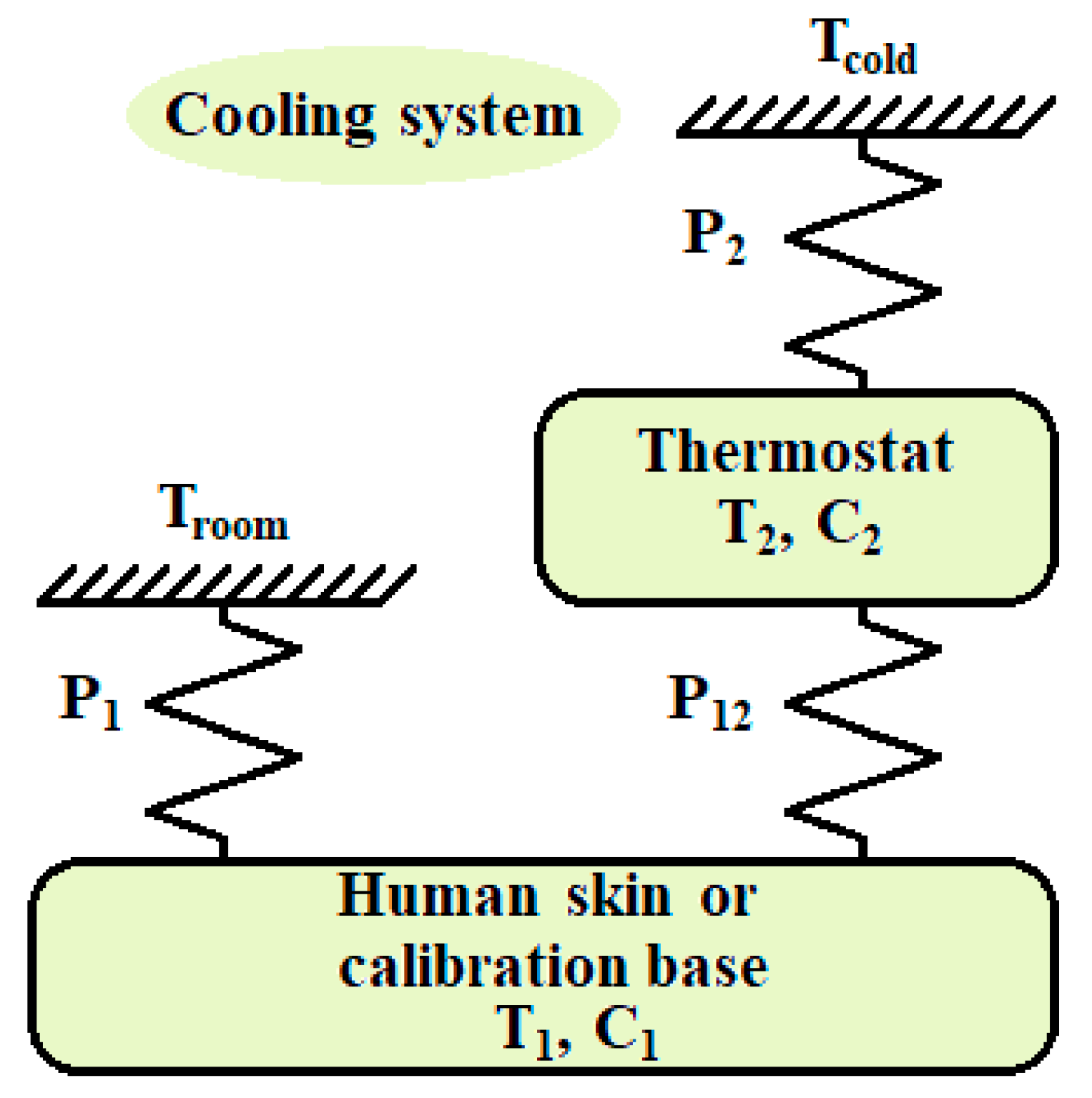
2.2. Calorimetric Model

The device is modelled as a two-inputs, two-outputs system. The inputs are the power that passes through the sensor and that is to be measured (W1), and the power dissipated in the thermostat (W2) that maintains the programmed temperature of the thermostat. The outputs are the calorimetric signal (y) and the thermostat temperature (T2).
The signal-to-noise ratio of the output signals in an experimental measurement on human skin varies from 300 to 3000, (50 dB to 70 dB). This signal-to-noise ratio allows the identification of up to two poles of the transfer functions (TFs) that link the inputs to the outputs. For this reason, a simple two-element model is proposed (Figure 2). This modelling, called localized constants, is frequently used in heat conduction calorimeters [30,31,32]. The first element represents the domain where the heat dissipation to be measured takes place (W1). When the sensor is applied to the human body, this domain is the human skin. When the sensor is in the calibration base, this domain is the copper plate where the Joule calibration resistor is located. The second element represents the thermostat. The power dissipated in this domain (W2) is determined by a PID controller that holds the programmed temperature. The elements have C1 and C2 heat capacities. As the thermal conductivity of these elements is infinite, this implies considering a temperature in each domain (T1 and T2). These elements are thermally coupled to the outside and to each other by P12, P1 and P2 thermal conductance couplings. The outside is configured by the environment that is at a Troom temperature, and the cooling system that is at a Tcold temperature (see Figure 2).
The power developed in each element (W1 and W2) is equal to the accumulated heat power in the domain plus the power transmitted by conduction to the neighbouring domains. The following equations (Equation (1)) describe the energy balance that relates the powers to the temperatures of each domain [19].
W 1 ( t ) = C 1 d T 1 d t + P 1 ( T 1 T r o o m ) + P 12 ( T 1 T 2 ) W 2 ( t ) = C 2 d T 2 d t + P 2 ( T 2 T c o l d ) + P 12 ( T 2 T 1 )
The calorimetric signal is a linear combination of the temperatures of the bodies that are in contact with each face of the measuring thermopile. That is, y = k(T1T2).
Considering that the ambient temperature and the temperature of the cold focus (Troom and Tcold) are constant during the measurement and correcting the baselines of the variables (T1, T2, W1 and W2), we obtain an equivalent system of equations (Equation (2)) in which Troom and Tcold do not appear. In this case the values of the curves ΔT1, ΔT2, Δy, ΔW1 and ΔW2 are zero at the initial instant [19].
Δ W 1 ( t ) = C 1 d Δ T 1 d t + P 1 Δ T 1 + P 12 ( Δ T 1 Δ T 2 ) Δ W 2 ( t ) = C 2 d Δ T 2 d t + P 2 Δ T 2 + P 12 ( Δ T 2 Δ T 1 ) ;     Δ y = k ( Δ T 1 Δ T 2 )
When the sensor is placed on its base, the ambient temperature Troom remains practically constant. However, when the sensor is applied to the skin there are two significant changes. The first one refers to C1; now, this element is not the base but the area of the skin where the dissipation is being measured. This heat capacity is unknown and different in each area of the human body. The second change is related to the ambient room temperature around the sensor. This temperature in the neighbourhood of the skin is higher than the ambient temperature in the environment of the base. When the baselines of the experimental curves are corrected, the initial situation is corrected, eliminating the terms Troom and Tcold at the base, but the “new ambient temperature” in the neighbourhood of human skin is not taken into account. Therefore, we assume that the ambient temperature in the vicinity of the skin is higher by a ΔT0 value.
We assume that this increase in temperature ΔT0 also affects the temperature of the cold focus, since Tcold = Troom + ΔTPeltier, where ΔTPeltier is the decrease in temperature produced by the cooling system. The value of ΔTPeltier depends on the supply voltage (VPeltier) of the thermopile and comes from Equation (3), whose parameters are determined experimentally [19,21].
Δ T P e l t i e r = a 0 + a 1 V P e l t i e r + a 2 V P e l t i e r 2
In our case, a0 =1.7 K, a1 = −9.2 KV−1; a2 = 1.0 KV−2. In each measure VPeltier is constant and consequently ΔTPeltier is also constant. Thus, if there is a change in Tcold, it is due only to changes in Troom. When the sensor is placed on the skin, the outer surface of the thermal insulation maintains the initial temperature and gradually adapts to the new situation. This thermal adaptation of the surface is not instantaneous, and in the calculation, we will assume that this adaptation follows a variation given by (Equation (4)). The validity of this expression is checked by adjusting the experimental curves with the curves determined by the model.
Δ T 0 = A ( 1 e t / τ T ) + B ( t / t e n d )
The parameters A, B and the time constant τT are determined in each measurement. Time (t) begins when the sensor is applied to the skin and ends (tend) when the sensor is placed back on its base. The new equations (Equation (5)) incorporate this variation in the ambient temperature (ΔT0).
Δ W 1 ( t ) = C 1 d Δ T 1 d t + P 1 Δ T 1 + P 12 ( Δ T 1 Δ T 2 ) P 1 Δ T 0 Δ W 2 ( t ) = C 2 d Δ T 2 d t + P 2 Δ T 2 + P 12 ( Δ T 2 Δ T 1 ) P 2 Δ T 0 ;     Δ y = k ( Δ T 1 Δ T 2 )
By sorting this system of equations, and applying and operating the Laplace transform, six TFs (Equation (6)) are obtained that relate the inputs ΔW1(s), ΔW2(s) and ΔT0(s) with the outputs ΔY(s) and ΔT2(s), where s is the Laplace variable. It is assumed that the initial value of all variables is zero and its derivative at the time origin is also zero and, for this reason, it is important to have a good initial baseline.
( Δ Y ( s ) Δ T 2 ( s ) ) = ( k C 2 s + P 2 Q ( s ) k C 1 s + P 1 Q ( s ) k ( P 1 C 2 P 2 C 1 ) s Q ( s ) P 12 Q ( s ) C 1 s + P 12 + P 1 Q ( s ) P 2 ( C 1 s + P 12 + P 1 ) + P 1 P 12 Q ( s ) ) ( Δ W 1 Δ W 2 Δ T 0 )   being ,   Q ( s ) = ( C 1 s + P 1 + P 12 ) ( C 2 s + P 2 + P 12 ) P 12 2
As can be seen in (Equation (6)), the denominators of the six TFs are the same, which implies that the poles of all the TFs are the same. However, the numerators of each TF are different. It can be verified that the transient response of the calorimetric signal and the temperature of the thermostat depend on the heat capacity C1 where dissipation occurs. In general, an increase in C1 implies higher values of the time constants, which results in a slower transient response. Nevertheless, this will be discussed further in the simulation section.

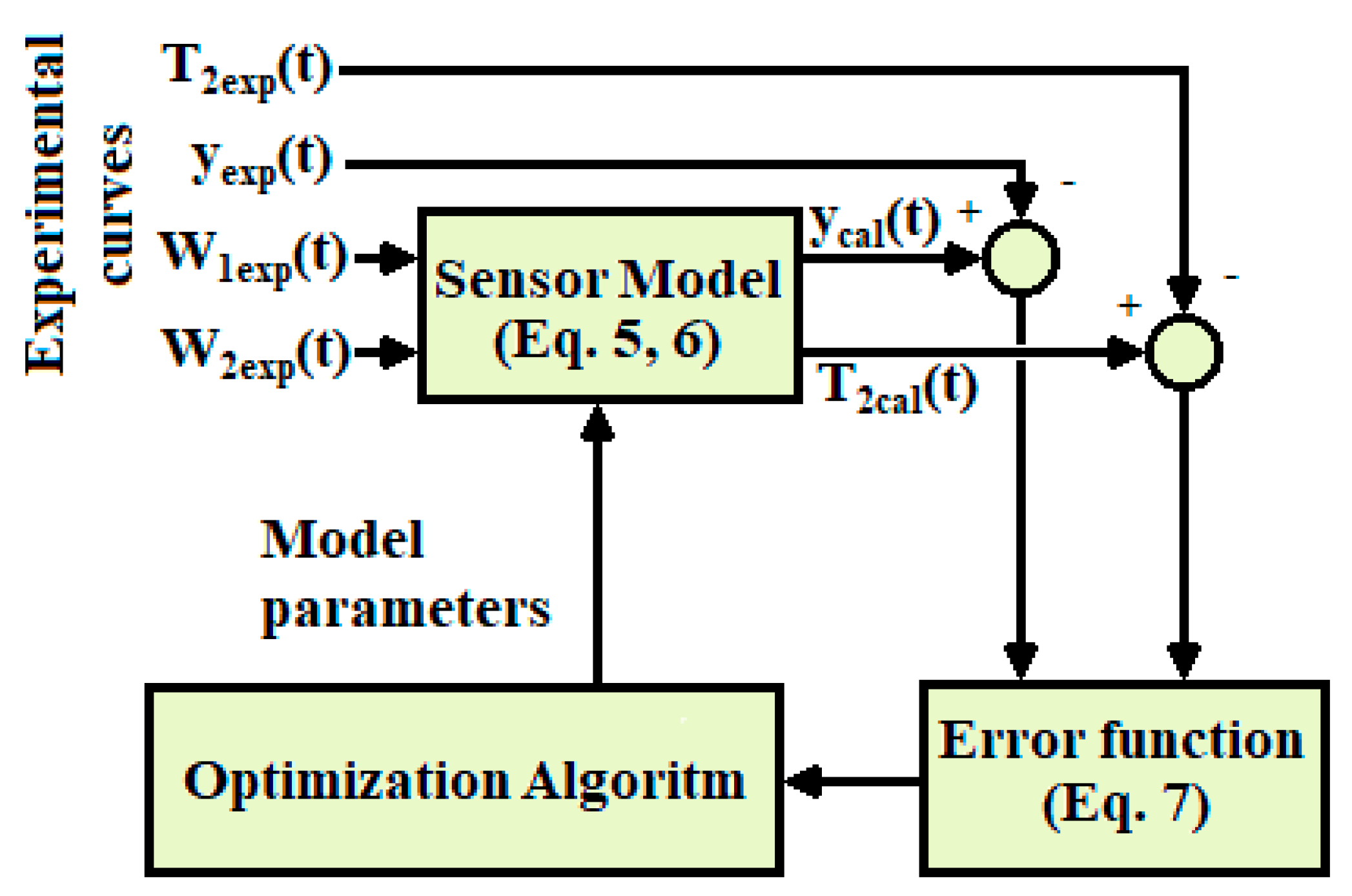
2.3. Identification of the Model

The hypothesis proposed in the model implies that the parameters C2, P1, P12, P2 and k are characteristic of the sensor and invariant. On the other hand, the calorimetric signal (y), the temperature of the thermostat (T2) and the power dissipated in the thermostat (W2) are known. However, C1 depends on the area where dissipation W1 takes place. This power W1 is only known when performing calibration measurements: these measurements allow determining the invariant parameters of the model.
For calibration, the sensor is placed on its base and measurements similar to those made on human skin are programmed. Initially, a constant temperature of the thermostat T20 is programmed, and when the steady state is reached, a constant power W10 in the base is dissipated for 300 s. Then, for 150 s, a linear increase in the thermostat temperature is programmed until T2end and simultaneously the dissipation in the base is linearly decreased from W10 to W1end. Finally, and for 300 s, the temperature of the thermostat T2end is kept constant, also keeping the dissipation W1end constant.
In Figure 3 the experimental curves of the input powers (W1 and W2) and the experimental curves of the output signals are represented: the calorimetric signal (y) and the thermostat temperature (T2). Two cases are shown: in the first one (green curves) the temperature increase in the thermostat is 10 K (from 26 to 36 °C); and in the second case (blue curves) the increase is 5 K (from 26 to 31 °C). In both cases the power W1 dissipated at the base (red curve) is 300 mW at the beginning and 100 mW at the end.
A minimization method based on the Nelder–Mead simplex algorithm [33,34,35] is used to identify the model parameters. The error criterion used is the sum of the roots of the root mean square errors (RMSE), weighted (Equation (7)). The root mean square error is calculated with the experimental curves (subscript exp) and those calculated by the model (subscript cal).
N is the number of points and α is a weighting coefficient (N = 1800, α = 4). The calculated curves are determined with the system of equations (Equation (6)). The sampling period is 0.5 s.
ε = ε y + α ε T 2 = 1 N i = 1 N ( y exp [ i ] y c a l [ i ] ) 2 + α N i = 1 N ( T 2 , exp [ i ] T 2 , c a l [ i ] ) 2
The calculation starts with some initial values of the model parameters (C1, C2, P1, P2, P12 and k). With these parameters the TFs that relate the inputs to the outputs (Equation (6)) are constructed, and the outputs calculated with the model (ycal and T2cal) are determined for the known inputs W1 and W2. Then the error criterion is applied (Equation (7)) and the Nelder–Mead method that provides new parameter values (C1, C2, P1, P2, P12 and k) is applied. The iterative process decreases the error (Equation (7)) until the fit between the calculated and experimental curves cannot be further improved. Figure 4 shows a diagram of the calculation procedure.
Table 1 shows the values of the parameters (C1, C2, P1, P2, P12, k) obtained in the calibration measurements. These results correspond to a series of 20 measurements in which the power dissipated in the base (400, 300 and 100 mW) and the increase in temperature of the thermostat (5 and 10 K) have been varied. The maximum RMSE in the calorimetric signal fittings is 14 µV over a 100mV peak-to-peak signal; and 4 mK on a 10 K peak-to-peak signal at the thermostat temperature fitting.

2.4. Simulation

Calibration of the sensor allows determining the model parameters that best fit the experimental measurements (Table 1). In this section the operation of the sensor is studied from simulations. (Equation (8)) shows the relationship between the inputs and outputs of the model by means of six transfer functions (TFi) whose expressions are indicated in the system of equations in (Equation (6)).
( Δ Y ( s ) Δ T 2 ( s ) ) = ( T F 1 ( s ) T F 2 ( s ) T F 3 ( s ) T F 4 ( s ) T F 5 ( s ) T F 6 ( s ) ) ( Δ W 1 Δ W 2 Δ T 0 )

2.4.1. Variation of the FT of the Model Depending on the Heat Capacity

A comparison of the TF is presented for different values of heat capacity. Figure 5 and Figure 6 represent the modulus of each TFi as a function of frequency, for extreme cases of heat capacity C1 = 3 JK−1 and C1 = 9 JK−1. The normalized module is represented to compare the dynamic responses with the same vertical scale.
In the calorimetric response, we observe that when C1 increases, the system responds slower, which is verified in TF1 and TF3; however, the dynamics of TF2 remains unchanged. On the other hand, the dynamic response of the thermostat temperature is less affected with the variation of C1, but as expected, the response of TF4 is slower with increasing values of C1. TF5 and TF6 are less altered with the variation of C1.

2.4.2. Simulations in the Calibration Base and in the Human Body

The simulations are performed from the systems of equations (Equation (5) or Equation (6)). First, we simulate the operation of the sensor when it is located in its base, which is completed for different heat capacities of the base: C1 = 3, 6 and 9 JK−1. The thermostat temperature is kept constant; when the sensor reaches steady state, it increases linearly to +10 K for 150 s and finally remains constant until the end. At the base, a constant power of W1 = 0.3 W is dissipated for 300 s, and when the thermostat temperature increases, it decreases linearly until W1 = 0.1 W, which remains constant until the end of the simulation. Figure 7 shows the thermostat temperature (T2), the calorimetric signals (y), the power dissipated in the base (W1) and the power dissipated in the thermostat (W2). Additionally, a 0.5 K linear increase in ambient temperature (ΔT0) has also been simulated. As expected, a higher value of the heat capacity C1 implies a slower transient response of the calorimetric signal.
Figure 8 shows the simulation of a measurement on the surface of the human body. The simulation takes into account that the sensor is initially at its base (C1 = 3 JK−1) and then it is applied to the skin, which has the same or different C1 heat capacity. When placing the sensor on the skin, three phenomena appear that make this measurement different from a calibration measurement at its base:
(1)
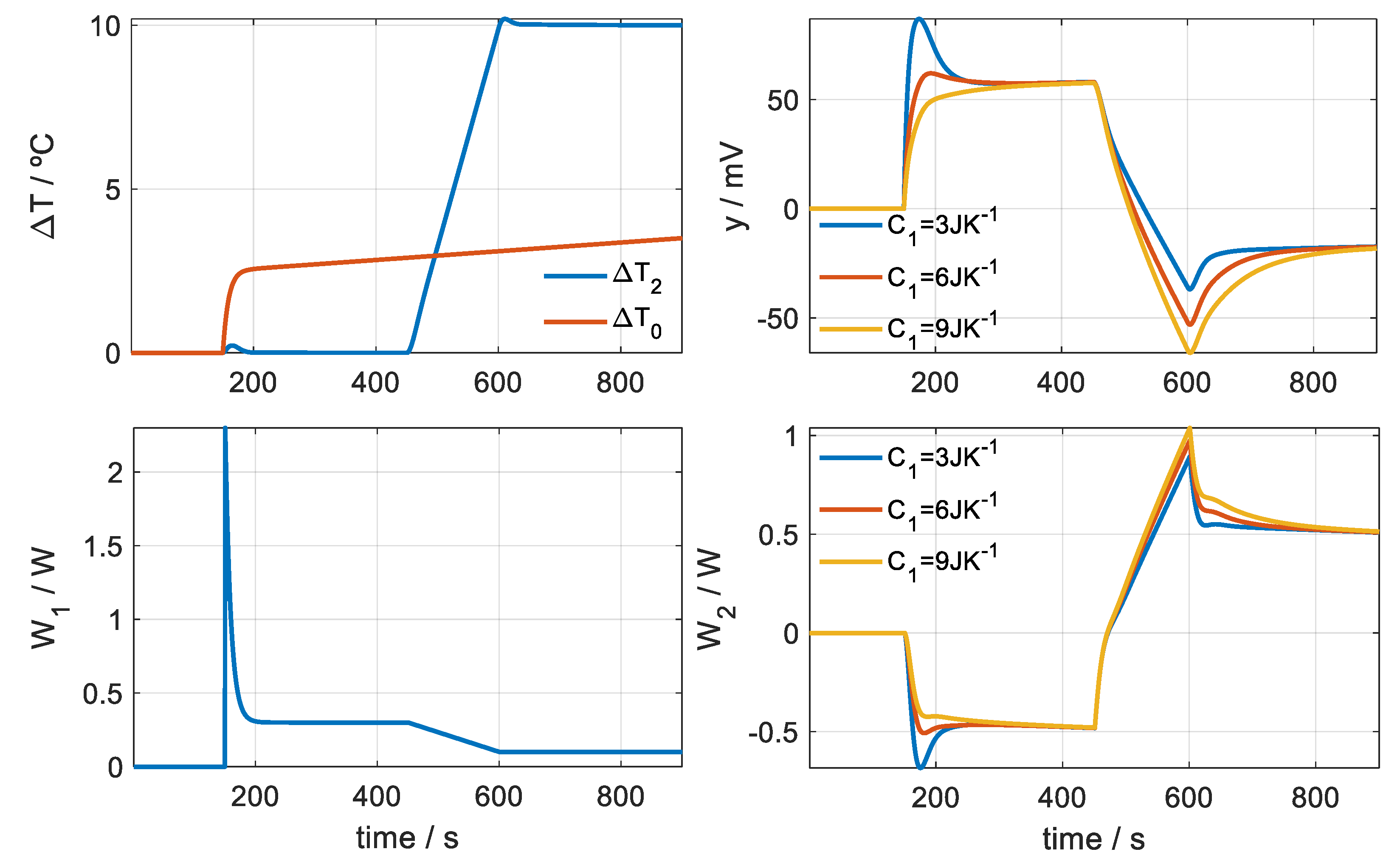
There is an instantaneous contact between the sensor surface and the skin surface that are at different temperatures. This produces a peak in the calorimetric signal, caused by an instantaneous power that is transmitted from the highest temperature surface to the lowest temperature. This instantaneous power that is transmitted from the skin to the sensor is represented with an exponential function of the form
W 1 ( t ) = A 0 + A 1 exp ( t / τ 1 )
where A0 is the power transmitted in steady state and A1 is the amplitude of the decreasing exponential due to instantaneous contact between the sensor surfaces and the skin. In the simulated case represented in Figure 8, we assume a power of A0 = 0.3 W for the initial temperature of the thermostat and a power of A0 = 0.1 W for the final temperature. We assume an amplitude of A1 = 2 W and a time constant of τ1 = 9 s.
(2)
The temperature surrounding the sensor has changed and is not the same temperature surrounding the sensor when it is in the base. In general, the temperature in the neighbourhood of the skin is higher. This temperature difference is represented by ΔT0 and responds to the expression given by (Equation (4)). In the simulated case A = 2.5 K, B = 1 K and a time constant of 9 s are considered.
(3)
The skin has a heat capacity typical of the area where it is being measured and therefore the transient response will depend on that heat capacity. Figure 8 shows these differences in the calorimetric signal. Three heat capacities for the skin have been used in the simulation: 3, 6 and 9 JK−1.

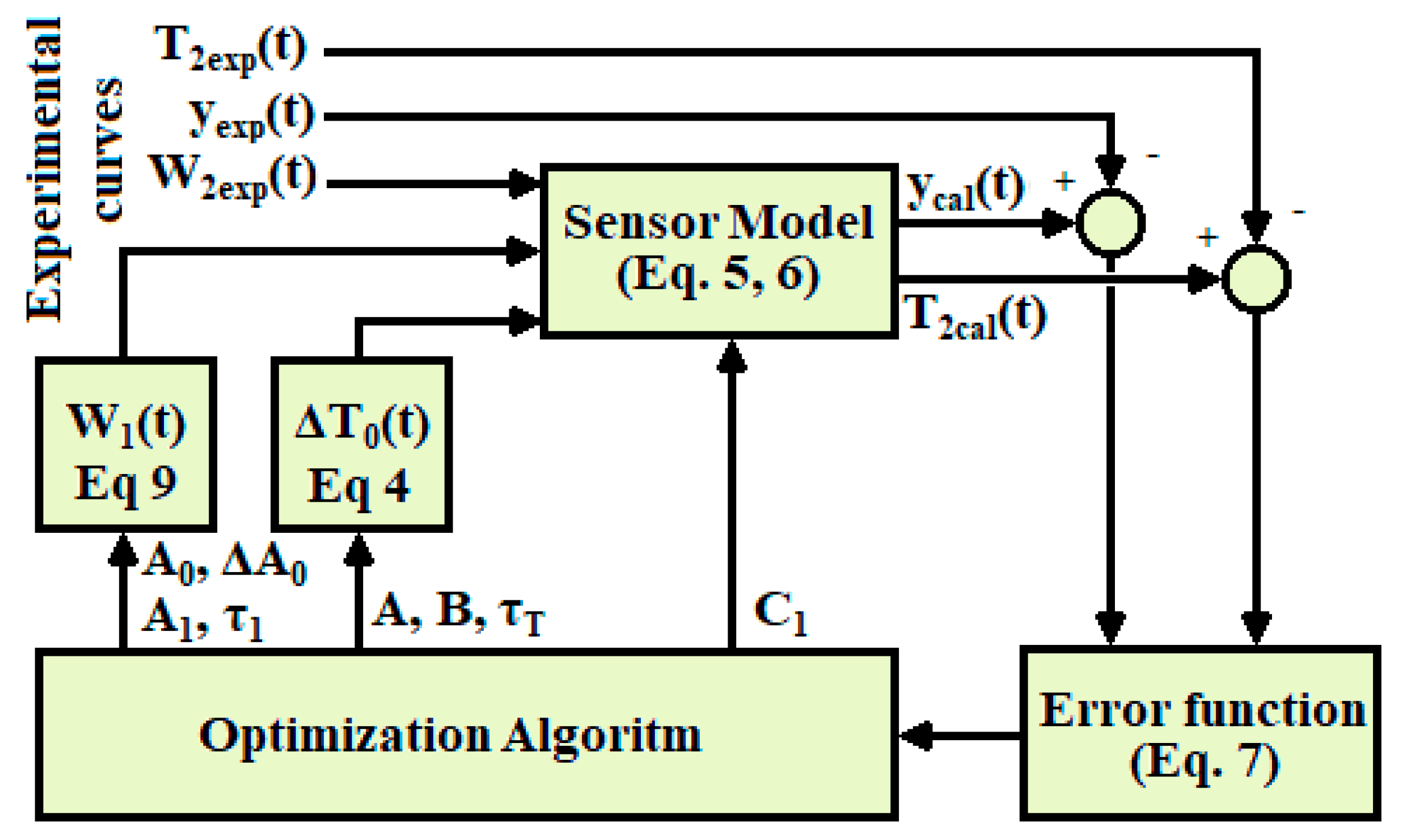
2.5. Method for Determining Heat Flux and Heat Capacity

This section describes the calculation method to determine the heat capacity and heat flow on a localized surface of the human body. The effectiveness of this method is verified from the curves simulated in the previous section. The following hypotheses are considered in the simulation of measurements on human skin:
(1)
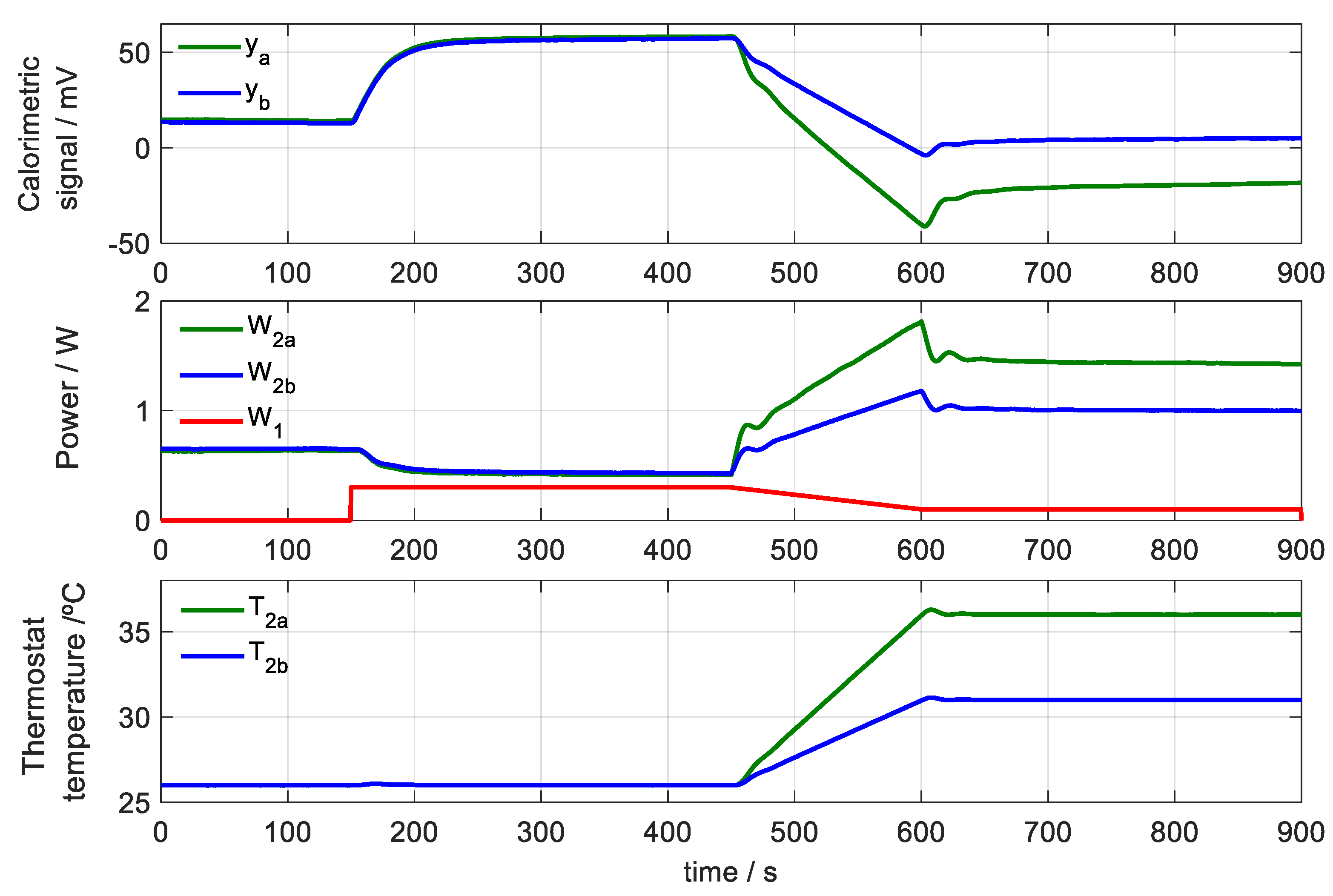
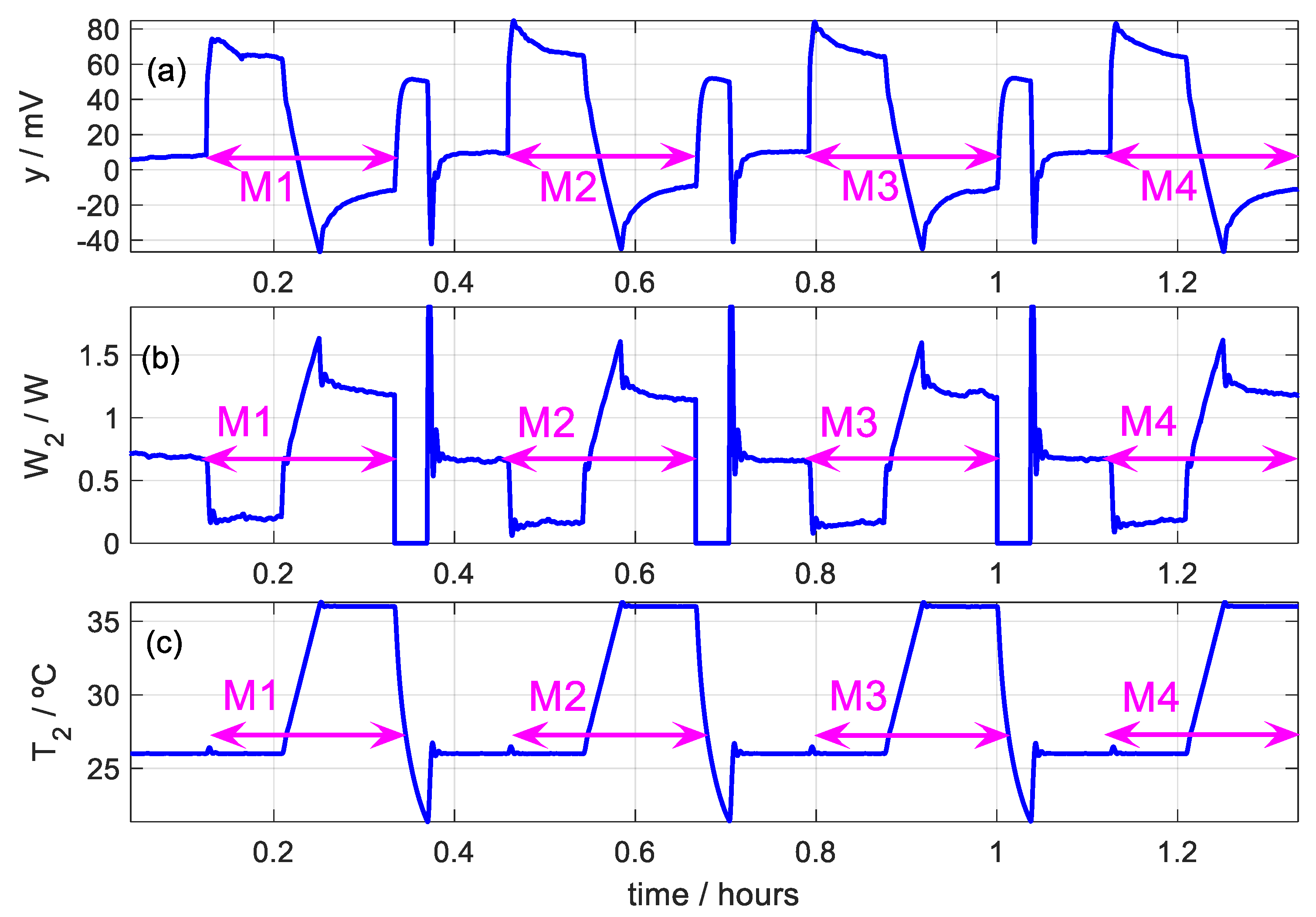
When the temperature of the thermostat is constant (T2initial) and the sensor is applied to the skin, the heat flow W1 that passes through the sensor obeys (Equation (9)). Contrastingly, when there is a linear variation in the temperature of the thermostat (from T2initial to T2end), we assume that the power W1 decreases linearly to a final value, which remains constant while the temperature of the thermostat remains constant at its final value (T2end). Thus, the heat flux can be described with (Equation (10)):
W 1 ( t ) = 0 f o r   t < t 1   W 1 ( t ) = A 0 + A 1 exp ( ( t t 1 ) / τ 1 ) f o r   t 1 t t 2 W 1 ( t ) = W 1 ( t 2 ) + Δ A 0 ( t t 2 ) / ( t 3 t 2 ) f o r   t 2 t t 3 W 1 ( t ) = W 1 ( t 3 ) f o r   t 3 t t e n d
In this equation, t1 is the instant in which the sensor is applied to the skin, t2 is the instant in which the linear increase in the temperature of the thermostat begins, t3 is the instant in which the aforementioned linear variation ends and starts to keep the temperature constant, and tend is the final instant of the measurement.
(2)
The difference in ambient temperature ΔT0 obeys (Equation (4)).
(3)
The relationships between all the system variables obey the equations of the model (Equation (5)). The model parameters have been determined in the calibration (Table 1) except for the value of C1 which depends on the place of measurement.
The chosen calculation method is similar to that used in model identification and discussed in Section 2.3 of this work. The method consists of determining eight parameters: the first four (A0, A1, τ1, ΔA0) allow us to reconstruct the power W1(t). The next three (A, B, τT) allow us to build the function ΔT0, and the last one (C1) completes the model described by (Equation (5)).
The procedure begins with initial values of the first seven parameters with which the curves W1(t) (Equation (9)) and ΔT0(t) (Equation (4)) are constructed. From these temporal functions, the power W2(t) (known) and the initial value of the eighth parameter (C1), the temperature and calorimetric curve of the thermostat are reconstructed using the system of equations (Equation (5)). From these reconstructions, the error criterion given by Equation (7)) is determined. Using the Nelder–Mead simplex algorithm [33,34,35], the new parameter values are determined. Figure 9 shows a diagram of the calculation procedure.
Table 2 shows the results obtained for the three simulated measurements represented in Figure 8. The errors in the determination of the heat flow A0 and ΔA0 are less than 0.3%, and in the determination of the heat capacity it is less than 0.4%. The errors (RMSE) in adjusting the calorimetric signal and the thermostat temperature (less than 9 µV and 0.15 mK) are very small in relation to the peak-to-peak value of these curves (120 mV and 10 K). These results on the simulated measurements demonstrate that the proposed method is adequate.

3. Results

In this section the results corresponding to measurements carried out on two healthy subjects are presented, the characteristic data of both subjects are indicated in Table 3. Both subjects are healthy, although the senior subject suffers from Hashimoto’s thyroiditis and is currently receiving treatment.

3.1. Measurements in the Junior Subject

Once the suitability of the method in Section 2.5 has been verified, the proposed method is applied to an experimental measurement on human skin. We present a measurement made on the temple of the junior subject. The subject is sitting and resting during the measurement. Four identical consecutive measurements are made. Each of them is of the same type as those performed in the simulation. Figure 10 shows the experimental curves of the calorimetric signal (y), power dissipated in the thermostat (W2) and temperature of the thermostat (T2). Figure 11 shows the placement of the sensor on the subject’s temple. The measurements were made in the laboratory with an ambient temperature of 22.6 °C and a relative humidity of 53%.
We apply the calculation method to each measurement. The results obtained are shown in Table 4 where the values of the eight parameters are indicated. Firstly, the parameters (A0, A1, τ1, ΔA0) related to the reconstruction of the heat flow through the sensor as a function of time when applied to human skin. Next, the value of the heat capacity of the area of the human body where the measurement is made is observed, the obtained average value being 5.91 JK−1. Finally, the parameters (A, B, τT) that allow us to reconstruct ΔT0, which is the equalization of the temperature around the sensor when it is applied to human skin, are obtained. Adjustment errors are less than 35 µV for a 120 mV peak-to-peak calorimetric signal, and 4 mK for a 10 K peak-to-peak thermostat temperature.
Figure 12a shows the heat flow measured by the sensor in the first measurement made on the subject’s temple. The initial transient can be observed when applied from the sensor due to the instantaneous contact between the sensor surfaces and the skin. Next, the heat flow reaches a steady state of 288 mW for the thermostat temperature of 26 °C. This power decreases linearly as the thermostat temperature increases, reaching a value of 67 mW for the thermostat temperature of 36 °C. The reconstruction of the calorimetric signal and the thermostat temperature can be seen in Figure 12b, while Figure 12c displays the experimental and calculated curves indicated with the subscripts exp and cal, respectively. The variation ΔT0 as a function of time is also represented in Figure 12c.
The power dissipated by the subject depends on the physical situation of the subject, the ambient, the temperature and the humidity, among other factors. We consider that a rigorous thermal characterization of the skin requires, in addition to knowledge of heat flow, data on the heat capacity and thermal conductance of the skin. The heat capacity and heat flux are determined directly by the calculation method. Thermal conductance (or inverse, thermal resistance), can be characterized from the variation of heat flow with the temperature of the thermostat. The inverse of the slope of this line has units of thermal resistance, therefore we define an equivalent thermal resistance of the skin Rskin with the expression given by (Equation (11)).
R s k i n = Δ T 2 Δ W 1 R s e n s o r
The thermal resistance of the sensor Rsensor is the inverse of the thermal conductivity P12. In this case, Rsensor = 1/P12 = 10.41 K/W, ΔT2 = 10 K, ΔW1 = ΔA0. Substituting the values from Table 4, we obtain Rskin = 36.5 ± 1.7 K/W. The uncertainty of the values obtained for the thermal properties of the skin in this series of measurements is 3.5% for heat capacity and 4.7% for equivalent thermal resistance.

3.2. Measurements in Senior Subject

In this section, eight measurements performed on different days in the temple of the healthy 62 year-old male are presented. Table 5 shows the results obtained. Figure 13 shows the variation of the heat flow of each day as a function of time and the temperature of the thermostat. The heat flow is very similar on both days, although on the first day it is slightly higher. This could be because the ambient temperature is lower, which produces greater dissipation. As for the thermal properties of the skin in the measured area, the average heat capacity obtained on the first day is 5.7 J/K, on the second day it is 5.9 J/K, and the mean value is C1 = 5.8 ± 0.2 J/K. The average equivalent thermal resistance obtained on the first day is 31 K/W, on the second day it is 29 K/W, and the average value between the two days is 30 ± 2 K/W. The uncertainty in determining the thermal properties of the skin is 3.4% for heat capacity and 6.7% for thermal resistance.
Table 6 shows results of two series of measurements performed on the right hand on two different days. In this case there, is a clear difference in the series of measurements from the first day given that the subject had an unusually low dissipation. The temperature around the sensor in the first day is Troom + A = 21.3 + 0.61 = 21.91 °C, however, in the second day it is 23.68 °C. These values clearly show that the surface temperature of the skin is lower in the first case. On the other hand, we can compare the area A1τ1 which represents the over-energy of the transitory phenomenon. In the measurements of the first day, said energy is negative or very small compared to that of the second day. This is because the surface temperature of the skin before applying the sensor to the skin is lower on the first day. We also compared the heat capacities and equivalent thermal resistances obtained: on the first day C1 = 5.05 ± 0.20 JK−1, Rskin = 38.9 ± 0.7 KW−1, and on the second day C1 = 5.43 ± 0.49 JK−1, Rskin = 28.9 ± 1.3 KW−1. The heat capacities obtained in both measurements are less than in the temple and the values obtained in each day are of the same order of magnitude as those that occurred in the measurements made in the temple. Thus, we can consider an average heat capacity in the hand of 5.3 ± 0.4 J/K with an uncertainty of 8%. However, the equivalent thermal resistance obtained in these two measurements is clearly different, so that on the first measured day, with less heat dissipation, the equivalent thermal resistance is 35% greater than that obtained on the second day. With this discussion on the results obtained, we want to indicate that while the heat capacity in an area of the skin keeps its value in a range of ±8%, the thermal resistance can change greatly depending on the physical situation of the subject.

3.3. Discussion

The magnitude of equivalent thermal resistance and heat capacity exposed in this work is global and of non-specific values, and is associated with the measured 2 × 2 cm2 skin area. The coefficient of variation is 3.5% for heat capacity and 6% for equivalent thermal resistance. These indicators are similar to values obtained in other works [10,15,16]. To compare our values with those in the literature, it is necessary to consider the thermal penetration depth. In our case, this is 3–4 mm depending on the measured area. From this condition, the specific heat capacities and thermal conductivities obtained from our experimental results are consistent with the literature. For example, for a skin volume of 2 × 2 × 0.4 cm3, considering an average specific heat capacity of 3.40 Jg−1K−1 and an average density of 1.15 g/cm3 [36,37], we obtain an absolute heat capacity of 6.26 JK−1. For an average thermal conductivity of 0.30 Wm−1K−1 [36,37], the thermal resistance would be 33.3 KW−1. These values are similar to our results.
The results obtained in this work have been obtained from experimental measurements made with a previously calibrated instrument. A more precise interpretation of the experimental results requires a better study of the skin’s thermal model. An increase in thermal penetration depth implies an increase in the heat capacity and thermal resistance of the zone. Other variables that affect the thermal properties are the physical state of the subject and the presence of lesions in the measurement zone. The physical state of the subject significantly affects the equivalent thermal resistance and, to a lesser extent, the heat capacity.

4. Conclusions

In this work a calorimetric sensor has been used to measure, by applying it to the skin, the heat flow dissipated by the human body. A non-invasive method is proposed to determine the heat capacity and equivalent thermal resistance of the measured skin area. The modelling of the sensor is effective since it is capable of relating the signals measured by the sensor with the heat flow that passes through the sensor. A sensor calibration has been carried out to determine the invariant parameters of the model. A calculation method that allows one to reliably determine the heat flow and the thermal properties of the skin in the measured area has been proposed. We have verified that the heat capacity of the skin is a property whose value remains at a value that can vary by 8%. However, the equivalent thermal resistance of the skin has a greater variability due to its great dependence on the physical situation of the subject.
With this work, we show the ability of the sensor to determine in vivo the heat flow, the equivalent thermal resistance and the heat capacity of the skin using a non-invasive technique. These physical magnitudes show a great variability and depend on physiological and environmental factors. While this fact could be interpreted as a problem of uncertainty, it is an opportunity to advance the study of human physiology with new data provided by the sensor utilised in this work. The repeatability experiments made in each series show that the variability of the results responds more to changes in the subject and the environment than to changes in the device.
Manually clamping of the sensor on the skin is an inconvenience as it requires specialized personal. Currently, in order to determine the absolute values of the heat flow, it is necessary to transfer the sensor from its base to the skin, and this is carried out manually. However, for the determination of equivalent thermal resistance and heat capacity, it is not necessary for the sensor to be previously on the base; instead, it can be permanently placed on the skin by means of an adapted clamp. We are currently working on this possibility by thermally exciting the skin with sinusoidal thermal dissipations.

Author Contributions

F.S., M.R.d.R. (Manuel Rodríguez de Rivera) and P.J.R.d.R. contributed equally to the investigation. M.R.d.R. (Miriam Rodríguez de Rivera) contributed to the medical methodology of the work. G.M.C. contributed to the validation and supervision of the research. All authors have read and agreed to the published version of the manuscript.

Funding

This research was funded by the “Ministerio de Ciencia, Innovación y Universidades (Spain), grant number FPU18/02990. Grant holder: P.J.R.d.R. (pre-doctoral grant)”.

Conflicts of Interest

The authors declare no conflict of interest.

References

  1. Brooks, A.G.; Withers, R.T.; Gore, C.J.; Vogler, A.J.; Plummer, J.; Cormack, J. Measurement and prediction of METs during household activities in 35- to 45-year-old females. Eur. J. Appl. Physiol. 2004, 91, 638–648. [Google Scholar] [CrossRef] [PubMed]
  2. Taylor, N.A.S.; Tipton, M.J.; Kenny, G.P. Considerations for the measurement of core, skin and mean body temperatures. J. Therm. Biol. 2014, 46, 72–101. [Google Scholar] [CrossRef] [Green Version]
  3. Wiegand, N.; Naumov, I.; Nőt, L.G.; Vámhidy, L.; Lőrinczy, D. Differential scanning calorimetric examination of pathologic scar tissues of human skin. J. Therm. Anal. Calorim. 2013, 111, 1897–1902. [Google Scholar] [CrossRef]
  4. Mehdi, M.; Fekecs, T.; Zapf, I.; Fekecs, T.; Lőrinczy, D. Differential scanning calorimetry (DSC) analysis of human plasma in different psoriasis stages. J. Therm. Anal. Calorim. 2013, 111, 1801–1804. [Google Scholar] [CrossRef]
  5. Deng, Z.-S.; Liu, J. Blood perfusion-based model for characterizing the temperature fluctuation in living tissues. Physica A 2001, 300, 521–530. [Google Scholar] [CrossRef]
  6. Hassanpour, S.; Saboonchi, A. Modeling of heat transfer in a vascular tissue-like medium during an interstitial hyperthermia process. J. Therm. Biol. 2016, 62, 150–158. [Google Scholar] [CrossRef]
  7. Agrawal, M.; Pardasani, K.R. Finite element model to study temperature distribution in skin and deep tissues of human limbs. J. Therm. Biol. 2016, 62, 98–105. [Google Scholar] [CrossRef]
  8. Lee, E.K.; Kim, M.K.; Lee, C.H. Skin-Mountable Biosensors and Therapeutics: A Review. Annu. Rev. Biomed. Eng. 2019, 21, 299–323. [Google Scholar] [CrossRef]
  9. Liu, Y.; Wang, H.; Zhao, W.; Zhang, M.; Qin, H.; Xie, Y. Flexible, Stretchable Sensors for Wearable Health Monitoring: Sensing Mechanisms, Materials, Fabrication Strategies and Features. Sensors 2018, 18, 645. [Google Scholar] [CrossRef] [Green Version]
  10. Okabe, T.; Fujimura, T.; Okajima, J.; Aiba, S.; Maruyama, S. Non-invasive measurement of effective thermal conductivity of human skin with a guard-heated thermistor probe. Int. J. Heat Mass Tran. 2018, 126, 625–635. [Google Scholar] [CrossRef]
  11. Gunga, H.-C.; Werner, A.; Stahn, A.; Steinach, M.; Schlabs, T.; Koralewski, E.; Kunz, D.; Belavy, D.L.; Felsenberg, D.; Sattler, F.; et al. The Double Sensor—A non-invasive device to continuously monitor core temperature in humans on earth and in space. Respir. Physiol. Neurobiol. 2009, 169, S63–S68. [Google Scholar] [CrossRef] [PubMed]
  12. Mazgaoker, S.; Ketko, I.; Yanovich, R.; Heled, Y.; Epstein, Y. Measuring core body temperature with a non-invasive sensor. J. Therm. Biol. 2017, 66, 17–20. [Google Scholar] [CrossRef] [PubMed]
  13. Marchiori, B.; Regal, S.; Arango, Y.; Delattre, R.; Blayac, S.; Ramuz, M. PVDF-TrFE-Based Stretchable Contact and Non-Contact Temperature Sensor for E-Skin Application. Sensors 2020, 20, 623. [Google Scholar] [CrossRef] [PubMed] [Green Version]
  14. Gao, L.; Zhang, Y.; Malyarchuk, V.; Jia, L.; Jang, K.-I.; Webb, R.C.; Fu, H.; Shi, Y.; Zhou, G.; Shi, L.; et al. Epidermal photonic devices for quantitative imaging of temperature and thermal transport characteristics of the skin. Nat. Commun. 2014, 5, 4938. [Google Scholar] [CrossRef] [PubMed] [Green Version]
  15. Webb, R.C.; Pielak, R.M.; Bastien, P.; Ayers, J.; Niittynen, J.; Kurniawan, J.; Manco, M.; Lin, A.; Cho, N.H.; Malyrchuk, V.; et al. Thermal transport characteristics of human skin measured in vivo using ultrathin conformal arrays of thermal sensors and actuators. PLoS ONE 2015, 10, e0118131. [Google Scholar] [CrossRef]
  16. Tian, L.; Li, Y.; Webb, R.C.; Krishnan, S.; Bian, Z.; Song, J.; Ning, X.; Crawford, K.; Kurniawan, J.; Bonifas, A.; et al. Flexible and stretchable 3ω sensors for thermal characterization of human skin. Adv. Funct. Mater. 2017, 27, 1701282. [Google Scholar] [CrossRef]
  17. Jesús, C.; Socorro, F.; Rodríguez de Rivera, M. Development of a calorimetric sensor for medical application. Part III. Operating methods and applications. J. Therm. Anal. Calorim. 2013, 113, 1009–1013. [Google Scholar] [CrossRef]
  18. Jesús, C.; Socorro, F.; Rodríguez de Rivera, H.J.; Rodriguez de Rivera, M. Development of a calorimetric sensor for medical application. Part IV. Deconvolution of the calorimetric signal. J. Therm. Anal. Calorim. 2014, 116, 151–155. [Google Scholar] [CrossRef]
  19. Socorro, F.; Rodríguez de Rivera, P.J.; Rodríguez de Rivera, M. Calorimetric minisensor for the localized measurement of surface heat dissipated from the human body. Sensors 2016, 16, 1864. [Google Scholar] [CrossRef] [Green Version]
  20. Socorro, F.; Rodríguez de Rivera, P.J.; Rodríguez de Rivera, M.; Rodríguez de Rivera, M. Mathematical model for localised and surface heat flux of the human body obtained from measurements performed with a calorimetry minisensor. Sensors 2017, 17, 2749. [Google Scholar] [CrossRef] [Green Version]
  21. Rodríguez de Rivera, P.J.; Rodríguez de Rivera, M.; Socorro, F.; Rodríguez de Rivera, M. Method for transient heat flux determination in human body surface using a direct calorimetry sensor. Measurement 2019, 39, 1–9. [Google Scholar] [CrossRef]
  22. Rodríguez de Rivera, P.J.; Rodríguez de Rivera, M.; Socorro, F.; Rodríguez de Rivera, M. Measurement of human body surface heat flux using a calorimetric sensor. J. Therm. Biol. 2019, 81, 178–184. [Google Scholar] [CrossRef]
  23. Rodríguez de Rivera, M.; Socorro, F. Baseline changes in an isothermal titration microcalorimeter. J. Therm. Anal. Calorim. 2005, 80, 769–773. [Google Scholar] [CrossRef]
  24. Lahiri, B.B.; Bagavathiaappan, S.; Jayakumar, T.; Philip, J. Medical applications of infrared thermography: A review. Infrared Phys. Technol. 2012, 55, 221–235. [Google Scholar] [CrossRef] [PubMed]
  25. Godoy, S.E.; Hayat, M.M.; Ramirez, D.A.; Myers, S.A.; Padilla, R.S.; Krishna, S. Detection theory for accurate and non-invasive skin cancer diagnosis using dynamic thermal imaging. Biomed. Opt. Express. 2017, 8, 2301–2323. [Google Scholar] [CrossRef] [PubMed] [Green Version]
  26. Haidar, S.G.; Charity, R.M.; Bassi, R.S.; Nicolai, P.; Singh, B.K. Knee skin temperature following uncomplicated total knee replacement. Knee 2006, 13, 422–426. [Google Scholar] [CrossRef] [PubMed]
  27. Rajapakse, C.; Grennan, D.M.; Jones, C.; Wilkinson, L.; Jayson, M. Thermography in the assessment of peripheral joint inflammation—A re-evaluation. Rheumatol. Rehabil. 1981, 20, 81–87. [Google Scholar] [CrossRef]
  28. Rokita, E.; Rok, T.; Taton, G. Application of thermography for the assessment of allergen-induced skin reactions. Med. Phys. 2011, 38, 765–772. [Google Scholar] [CrossRef]
  29. Vecchio, P.C.; Adebajo, A.O.; Chard, M.D.; Thomas, P.P.; Hazleman, B.L. Thermography of frozen sholder and rotator cuff tendinitis. Clin. Rheumatol. 1992, 11, 382–384. [Google Scholar] [CrossRef]
  30. Rodríguez de Rivera, M.; Socorro, F.; Dubes, J.P.; Tachoire, H.; Torra, V. Microcalorimetrie: Identification et déconvolotion automatique à l’aide de modéles physiques. Thermochim. Acta 1989, 150, 11–25. [Google Scholar] [CrossRef]
  31. Socorro, F.; Rodríguez de Rivera, M.; Jesús, C. A thermal model of a flow calorimeter. J. Therm. Anal. Calorim. 2001, 64, 357–366. [Google Scholar] [CrossRef]
  32. Auguet, C.; Lerchner, J.; Marinelli, P.; Martorell, F.; Rodríguez de Rivera, M.; Torra, V.; Wolf, G. Identification of micro-scale calorimetric devices IV. Descriptive models in 3-D. J. Therm. Anal. Calorim. 2003, 71, 951–966. [Google Scholar] [CrossRef]
  33. Lagarias, J.C.; Reeds, J.A.; Wright, M.H.; Wright, P.E. Convergence Properties of the Nelder-Mead Simplex Method in Low Dimensions. SIAM J. Opt. 1998, 9, 112–147. [Google Scholar] [CrossRef] [Green Version]
  34. Nelder, J.A.; Mead, C. A simplex method for function minimization. Comput. J. 1965, 7, 308–313. [Google Scholar] [CrossRef]
  35. Optimization ToolboxTM User’s Guide; 5th Printing; Revised for Version 3.0 (Release 14); The MathWorks, Inc.: Natic, MA, USA, June 2004.
  36. Cetingul, M.P.; Herman, C. A heat transfer model of skin tissue for the detection of lesions: Sensitivity analysis. Phys. Med. Biol. 2010, 55, 5933–5951. [Google Scholar] [CrossRef] [PubMed]
  37. McBride, A.; Bargmann, S.; Pond, D.; Limbert, G. Thermoelastic modelling of the skin at finite deformations. J. Therm. Biol. 2016, 62, 201–209. [Google Scholar] [CrossRef] [PubMed] [Green Version]
Figure 1. Diagram of the sensor in its calibration base. (1) aluminium plate, (2) measuring thermopile, (3) thermostat, (4) cooling thermopile, (5) aluminium heatsink, (6) fan, (7) thermal insulation, (8) calibration base (insulating material), (9) copper plate containing the calibration resistance, (10) magnets to hold the sensor in the base.
Sensors 20 03431 g001
Figure 2. Calorimetric sensor model.
Sensors 20 03431 g002
Figure 3. Experimental calibration measurements. Power dissipated in the base (W1), power dissipated in the thermostat (W2a and W2b), calorimetric signal (ya and yb) and temperature of the thermostat (T2a and T2b). The green curves represent the case of an increase of 10 K in temperature of the thermostat (from 26 to 36 °C), and the blue curves an increase of 5 K (from 26 to 31 °C). Troom = 23.4 °C.
Sensors 20 03431 g003
Figure 4. Model calculation procedure.
Sensors 20 03431 g004
Figure 5. Bode representation of the magnitude of the TFi that relates the calorimetric signal to the inputs of the calorimetric system.
Sensors 20 03431 g005
Figure 6. Bode representation of the magnitude of the TFi that relates the temperature of the thermostat with the inputs of the calorimetric system.
Sensors 20 03431 g006
Figure 7. Simulations for the case of calibrations on a base that has different heat capacities. Curve baselines have been corrected.
Sensors 20 03431 g007
Figure 8. Simulation of a measurement on human skin for different heat capacities of the skin. Curve baselines have been corrected.
Sensors 20 03431 g008
Figure 9. Heat capacity and heat flux calculation procedure.
Sensors 20 03431 g009
Figure 10. Series of four consecutive measurements (M1, M2, M3 and M4) performed on the temple of a healthy 28-year-old male subject (junior subject). (a) Calorimetric signal. (b) Power dissipated in the thermostat. (c) Thermostat temperature (Troom = 22.6 ± 0.5 °C, 53% RH).
Sensors 20 03431 g010
Figure 11. Sensor application to the skin.
Sensors 20 03431 g011
Figure 12. (a) Heat flow obtained from measurement M1 in Figure 10. (b) Adjustment of the calorimetric signal Δy. (c) Thermostat temperature fitting ΔT2 and representation of ΔT0.
Sensors 20 03431 g012
Figure 13. Heat flux transmitted from the temple to the sensor thermostat on different days and for different thermostat temperatures. Senior subject.
Sensors 20 03431 g013
Table 1. Model parameters (Figure 2 and (Equations (5) and (6)) obtained in the calibration measurements.
ParameterC1/JK−1C2/JK−1P1/mWK−1P2/mWK−1P12/mWK−1k/mVK−1
Mean3.003.9833.3864.8396.0719.02
SD0.110.102.773.917.191.09
SD: Standard deviation. Number of measurements: 20. Maximum RMSE: εy = 14 μV, εT2 = 4 mK (Equation (7))
Table 2. Results of the calculation on the simulated measurements with C1 = 3, 6 and 9 JK−1 (Figure 8).
Heat Flux
(Equation (9))
Model
(Equation (5))
ΔT0
(Equation (4))
Errors
(Equation (7))
A0/mWA1/mWτ1/sΔA0/mWC1/JK−1A/KB/KτTεy/µVεT/mK
(1)300.52125.98.4−200.33.012.510.999.08.880.13
(2)300.42125.58.4−200.56.002.500.999.04.700.09
(3)300.32123.68.4−200.68.982.500.999.03.290.08
Table 3. Data of the subjects.
SubjectGenderAgeWeight (kg)Height (m)
JuniorMale28671.72
SeniorMale62711.65
Table 4. Results in four consecutive measurements performed on the temple (junior subject, Figure 9).
MeasureHeat Flux
(Equation (9))
Model
(Equation (5))
ΔT0
(Equation (4))
Errors
(Equation (7))
A0/mWA1/Wτ1/sΔA0/mWC1/JK−1A/KB/KτTεy/µVεT/mK
M12882.737.9−2215.692.461.2316.629.71.47
M22793.248.1−2165.822.681.609.0033.52.03
M32723.388.0−2035.962.801.059.0034.73.78
M42723.827.0−2146.172.861.119.0029.12.55
Mean2783.297.8−2145.912.701.2510.9
SD7.60.450.57.60.210.180.153.80
Table 5. Results of measurements made on the temple in the senior subject on two different days (day 1: Troom = 23.3 °C, day 2: Troom = 23.5 °C).
Measure DayHeat Flux
(Equation (9))
Model
(Equation (5))
ΔT0
(Equation (4))
Errors
(Equation (7))
A0/mWA1/Wτ1/sΔA0/mWC1/JK−1A/KB/KτTεy/µVεT/mK
M11310.43.037.3−223.65.532.100.809.0024.42.59
M2325.94.895.3−251.26.082.411.469.0032.31.75
M3338.23.217.4−250.85.372.261.1630.032.62.00
M4324.83.557.0−241.35.912.570.6921.028.32.69
M12295.42.987.5−240.25.912.590.8430.029.21.15
M2316.42.829.1−253.25.832.450.819.0035.72.02
M3330.93.736.6−255.16.003.080.6030.025.81.54
M4340.13.298.0−276.45.852.711.0922.932.11.31
Table 6. Results of measurements made on the right hand in the senior subject in two different days (day 1: Troom = 21.3 °C, day 2: Troom = 21.8 °C).
Measure DayHeat Flux
(Equation (9))
Model
(Equation (5))
ΔT0
(Equation (4))
Errors
(Equation (7))
A0/mWA1/Wτ1/sΔA0/mWC1/JK−1A/KB/KτTεy/µVεT/mK
M1315.5−0.2715.0−202.05.080.610.499.3042.31.60
M212.9−0.03717.9−200.35.230.630.609.0023.61.96
M326.10.05510.7−205.84.830.930.939.8017.00.97
M14295.52.1146.9−248.44.851.880.969.0026.31.70
M2300.43.2176.4−247.26.041.960.7330.035.32.75
M3284.12.3357.7−259.85.501.730.719.6024.11.62
M4246.91.9358.3−263.75.311.430.819.0026.62.42

