A Detection and Tracking Algorithm for Resolvable Group with Structural and Formation Changes Using the Gibbs-GLMB Filter


Abstract
1. Introduction
2. Backgrounds
2.1. Labeled Random Finite Set (Labeled RFS)
2.2. Graph Theory
2.3. Graph Theory Model of Labeled RFS
2.4. Revolvable Group Tracking with Maneuver and the Efficient Implementation for the GLMB Filter
3. Analysis of the Structure and Formation of Discernible Group Targets
3.1. The Structure and Formation of Resolvable Group Targets
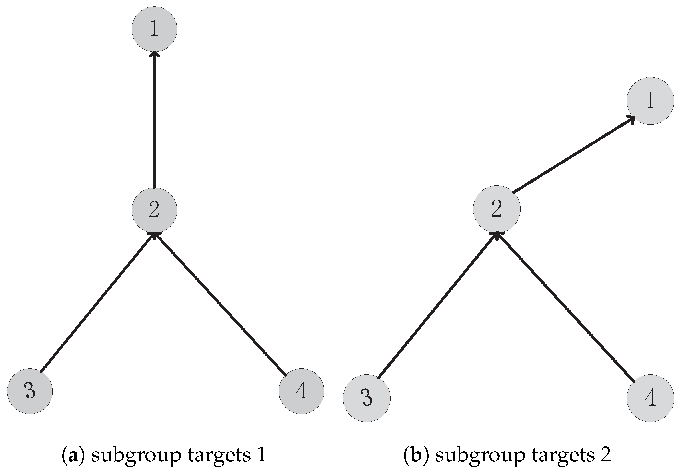
3.1.1. Structure
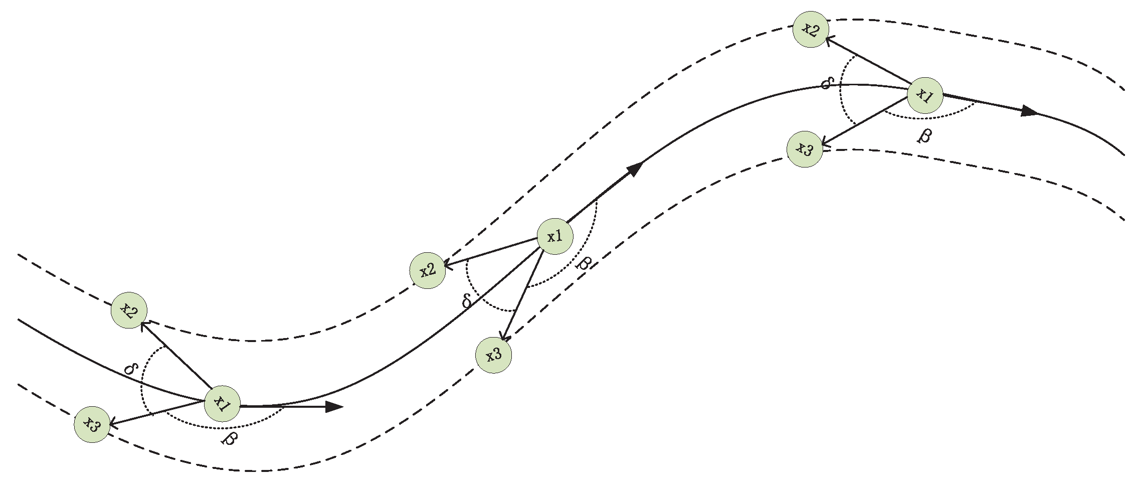
3.1.2. Formation
3.2. The Determination of Distinguishable Group Target Structure and Formation
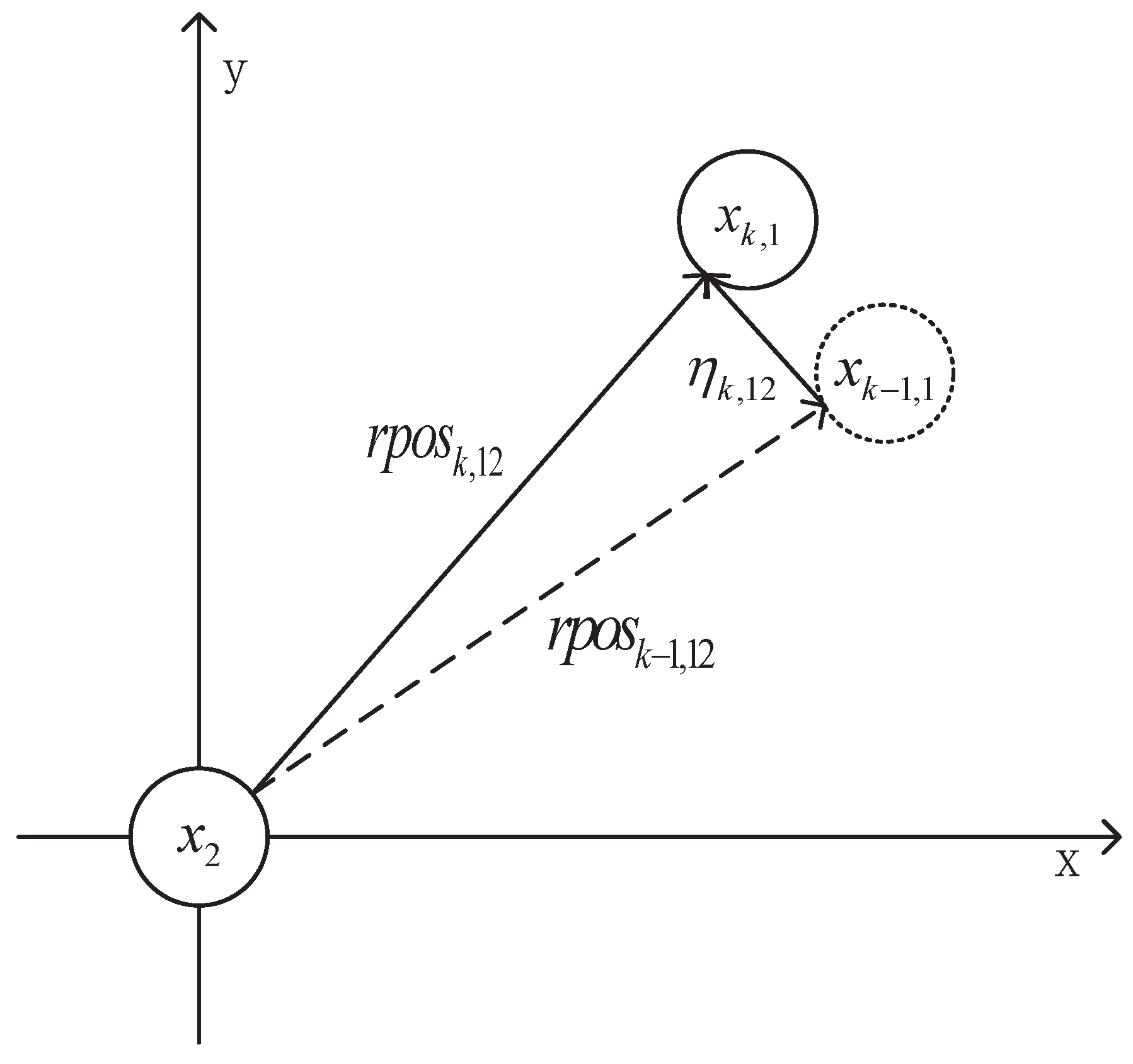
3.2.1. Determination of Group Target Structure in Continuous State
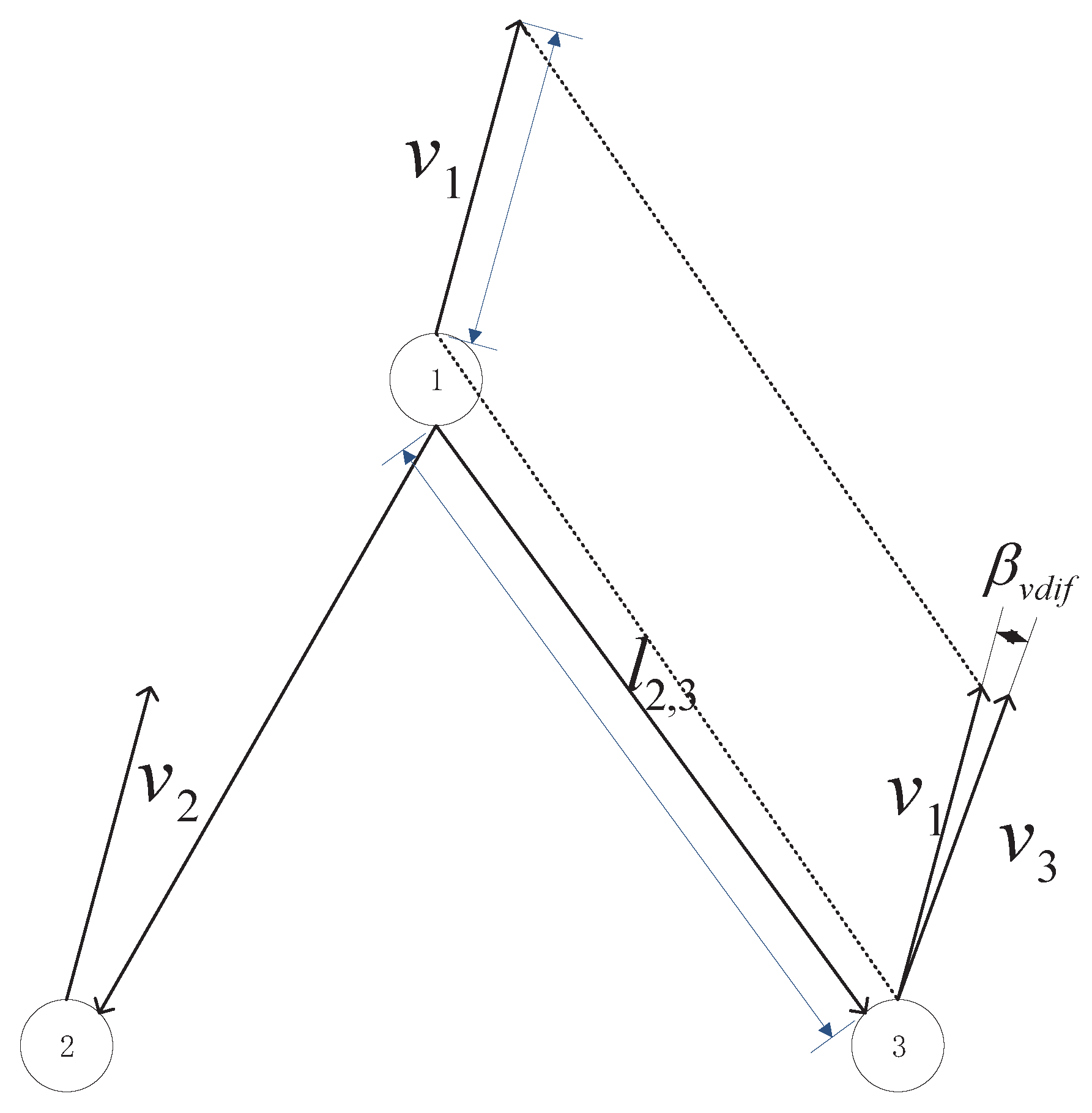
3.3. Determination of Group Target Formation in a Continuous State
4. Simulations
4.1. Experiment 1
4.1.1. Configuration Parameters for Experiment 1
4.1.2. The Result of the Experiment 1
4.2. Experiment 2
4.2.1. Configuration Parameters for Experiment 2
4.2.2. The Result of the Experiment 2
5. Conclusions
Author Contributions
Funding
Conflicts of Interest
References
- Clausen, U.; Klingner, M. Automated Driving: Computers take the wheel. In Digital Transformation; SpringVieweg: Berlin, Germany, 2019. [Google Scholar]
- Vo, B.N.; Dam, N.; Phung, D.; Tran, Q.N.; Vo, B.T. Model-based learning for point pattern data. Pattern Recognit. 2018, 84, 136–151. [Google Scholar] [CrossRef]
- Maggio, E.; Taj, M.; Cavallaro, A. Efficient multitarget visual tracking using random finite sets. IEEE Trans. Circuits Syst. Video Technol. 2008, 18, 1016–1027. [Google Scholar] [CrossRef]
- Meissner, D.; Reuter, S.; Dietmayer, K. Road user tracking at intersections using a multiple-model PHD filter. In Proceedings of the 2013 IEEE Intelligent Vehicles Symposium (IV), Gold Coast, QLD, Australia, 23–26 June 2013; pp. 377–382. [Google Scholar]
- Ristic, B.; Vo, B.N. Sensor control for multi-object state-space estimation using finite sets. Automatica 2010, 46, 1812–1818. [Google Scholar] [CrossRef]
- Ristic, B.; Vo, B.N.; Clark, D. A note on the reward function for PHD filters with sensor control. IEEE Trans. Aerosp. Electron. Syst. 2011, 47, 1521–1529. [Google Scholar] [CrossRef]
- Hoang, H.G.; Vo, B.T. Sensor management for multi-target tracking via multi-Bernoulli filtering. Automatica 2014, 50, 1135–1142. [Google Scholar] [CrossRef]
- Gostar, A.K.; Hoseinnezhad, R.; Bab-Hadiashar, A. Robust multi-Bernoulli sensor selection for multi-target tracking in sensor networks. IEEE Signal Process. Lett. 2013, 20, 1167–1170. [Google Scholar] [CrossRef]
- Hoang, H.G.; Vo, B.N.; Vo, B.T.; Mahler, R. The Cauchy–Schwarz divergence for Poisson point processes. IEEE Trans. Inf. Theory 2015, 61, 4475–4485. [Google Scholar] [CrossRef]
- Gostar, A.K.; Hoseinnezhad, R.; Bab-Hadiashar, A. Multi-Bernoulli sensor-selection for multi-target tracking with unknown clutter and detection profiles. Signal Process. 2016, 119, 28–42. [Google Scholar] [CrossRef]
- Gostar, A.K.; Hoseinnezhad, R.; Bab-Hadiashar, A.; Liu, W. Sensor-management for multitarget filters via minimization of posterior dispersion. IEEE Trans. Aerosp. Electron. Syst. 2017, 53, 2877–2884. [Google Scholar] [CrossRef]
- Beard, M.; Vo, B.T.; Vo, B.N.; Arulampalam, S. Void probabilities and Cauchy–Schwarz divergence for generalized labeled multi-Bernoulli models. IEEE Trans. Signal Process. 2017, 65, 5047–5061. [Google Scholar] [CrossRef]
- Fantacci, C.; Vo, B.N.; Vo, B.T.; Battistelli, G.; Chisci, L. Robust fusion for multisensor multiobject tracking. IEEE Signal Process. Lett. 2018, 25, 640–644. [Google Scholar] [CrossRef]
- Li, S.; Yi, W.; Hoseinnezhad, R.; Battistelli, G.; Wang, B.; Kong, L. Robust distributed fusion with labeled random finite sets. IEEE Trans. Signal Process. 2017, 66, 278–293. [Google Scholar] [CrossRef]
- Yi, W.; Li, S.; Wang, B. Computationally Efficient Distributed Multi-sensor Fusion with Multi-Bernoulli Filter. IEEE Trans. Signal Process. 2019, 68, 241–256. [Google Scholar]
- Papi, F.; Vo, B.N.; Vo, B.T.; Fantacci, C.; Beard, M. Generalized labeled multi-Bernoulli approximation of multi-object densities. IEEE Trans. Signal Process. 2015, 63, 5487–5497. [Google Scholar] [CrossRef]
- Papi, F.; Kim, D.Y. A particle multi-target tracker for superpositional measurements using labeled random finite sets. IEEE Trans. Signal Process. 2015, 63, 4348–4358. [Google Scholar] [CrossRef]
- Beard, M.; Reuter, S.; Granström, K.; Vo, B.T.; Vo, B.N.; Scheel, A. Multiple extended target tracking with labeled random finite sets. IEEE Trans. Signal Process. 2015, 64, 1638–1653. [Google Scholar] [CrossRef]
- Zhu, S.; Liu, W.; Cui, H. Multiple Resolvable GroupsTracking Using the GLMB Filter. Acta Autom. Sin. 2017, 43, 2178–2189. [Google Scholar]
- Beard, M.; Vo, B.T.; Vo, B.N. Bayesian multi-target tracking with merged measurements using labelled random finite sets. IEEE Trans. Signal Process. 2015, 63, 1433–1447. [Google Scholar] [CrossRef]
- Mahler, R. An introduction to Multisource-Multitarget Statistics And Applications; Lockheed Martin: Bethesda, MD, USA, 2000. [Google Scholar]
- Mahler, R.P. Multitarget Bayes filtering via first-order multitarget moments. IEEE Trans. Aerosp. Electron. Syst. 2003, 39, 1152–1178. [Google Scholar] [CrossRef]
- Goodman, I.R.; Mahler, R.P.; Nguyen, H.T. Mathematics of Data Fusion; Springer Science & Business Media: Dordrecht, The Netherlands; Boston, MA, USA; London, UK, 1997; Volume 37. [Google Scholar]
- Mahler, R.; Hall, D.; Llinas, J. Random Set Theory for Target Tracking and Identification. In In Data Fusion Handbook; CRC Press: Boca Raton, FL, USA, 2001. [Google Scholar]
- Panta K, C.D.E. Data association and track management for the gaussian mixture probability hypothesis density filter. IEEE Trans. Aerosp. Electron. Syst. 2009, 45, 1003–1016. [Google Scholar] [CrossRef]
- Mahler, R. PHD filters of higher order in target number. IEEE Trans. Aerosp. Electron. Syst. 2007, 43, 1523–1543. [Google Scholar] [CrossRef]
- Kumaradevan Punithakumar, T.K. A multiple-model probability hypothesis density filter for tracking maneuvering targets. Signal Data Process. Small Targets 2004, 44, 3553–3567. [Google Scholar] [CrossRef]
- Mahler, R.P. Statistical Multisource-Multitarget Information Fusion; Artech House: Norwood, MA, USA, 2007. [Google Scholar]
- Vo, B.T.; Vo, B.N.; Cantoni, A. The Cardinality Balanced Multi-Target Multi-Bernoulli Filter and Its Implementations. IEEE Trans. Signal Process. 2009, 57, 409–423. [Google Scholar] [CrossRef]
- Vo, B.T.; Vo, B.N. Labeled random finite sets and multi-object conjugate priors. IEEE Trans. Signal Process. 2013, 61, 3460–3475. [Google Scholar] [CrossRef]
- Vo, B.N.; Vo, B.T.; Phung, D. Labeled random finite sets and the Bayes multi-target tracking filter. IEEE Trans. Signal Process. 2014, 62, 6554–6567. [Google Scholar] [CrossRef]
- Vo, B.N.; Vo, B.T.; Hoang, H.G. An efficient implementation of the generalized labeled multi-Bernoulli filter. IEEE Trans. Signal Process. 2016, 65, 1975–1987. [Google Scholar] [CrossRef]
- Liu, W.; Chi, Y. Resolvable Group State Estimation with Maneuver Based on Labeled RFS and Graph Theory. Sensors 2019, 19, 1307. [Google Scholar] [CrossRef]
- Liu, W.; Zhong, C.; Wen, L. Multi-measurement target tracking by using random sampling approach. Acta Automatica Sinica 2013, 39, 164–174. [Google Scholar] [CrossRef]
- Zhu, S.; Liu, W.; Weng, C.; Cui, H. Multiple group targets tracking using the generalized labeled multi-Bernoulli filter. In Proceedings of the 2016 35th Chinese Control Conference (CCC), Chengdu, China, 27–29 July 2016. [Google Scholar]
- Liu, W.; Zhu, S.; Wen, C.; Yu, Y. Structure modeling and estimation of multiple resolvable group targets via graph theory and multi-Bernoulli filter. Automatica 2018, 89, 274–289. [Google Scholar] [CrossRef]
- Chen, L.; Liu, W. Finite mixture modeling and tracking algorithm based on GLMB filtering and Gibbs sampling. Acta Autom. Sin. 2019. [Google Scholar] [CrossRef]


| No. | 1 | 2 | 3 | 4 | 5 | 6 | 7 | 8 | 9 | 10 |
|---|---|---|---|---|---|---|---|---|---|---|
| precision | 78.57% | 64.71% | 84.62% | 68.75% | 64.71% | 81.82% | 73.33% | 78.57% | 73.33% | 78.57% |
| average | 74.70% | |||||||||
© 2020 by the authors. Licensee MDPI, Basel, Switzerland. This article is an open access article distributed under the terms and conditions of the Creative Commons Attribution (CC BY) license (http://creativecommons.org/licenses/by/4.0/).
Share and Cite
Ru, X.; Chi, Y.; Liu, W. A Detection and Tracking Algorithm for Resolvable Group with Structural and Formation Changes Using the Gibbs-GLMB Filter. Sensors 2020, 20, 3384. https://doi.org/10.3390/s20123384
Ru X, Chi Y, Liu W. A Detection and Tracking Algorithm for Resolvable Group with Structural and Formation Changes Using the Gibbs-GLMB Filter. Sensors. 2020; 20(12):3384. https://doi.org/10.3390/s20123384
Chicago/Turabian StyleRu, Xinfeng, Yudong Chi, and Weifeng Liu. 2020. "A Detection and Tracking Algorithm for Resolvable Group with Structural and Formation Changes Using the Gibbs-GLMB Filter" Sensors 20, no. 12: 3384. https://doi.org/10.3390/s20123384
APA StyleRu, X., Chi, Y., & Liu, W. (2020). A Detection and Tracking Algorithm for Resolvable Group with Structural and Formation Changes Using the Gibbs-GLMB Filter. Sensors, 20(12), 3384. https://doi.org/10.3390/s20123384