Statistical Analysis of Bistatic Radar Ground Clutter for Different German Rural Environments


Abstract
:1. Introduction
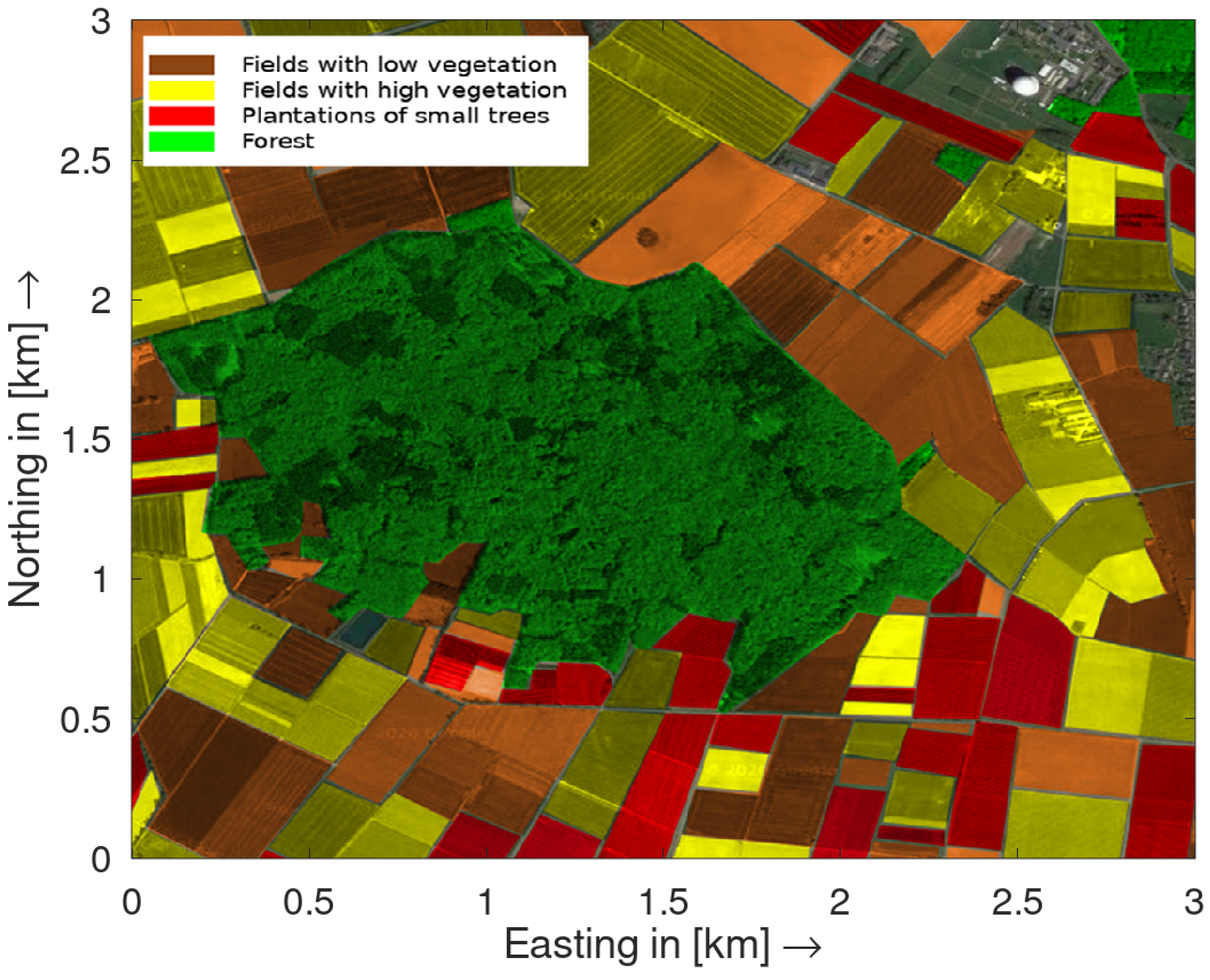
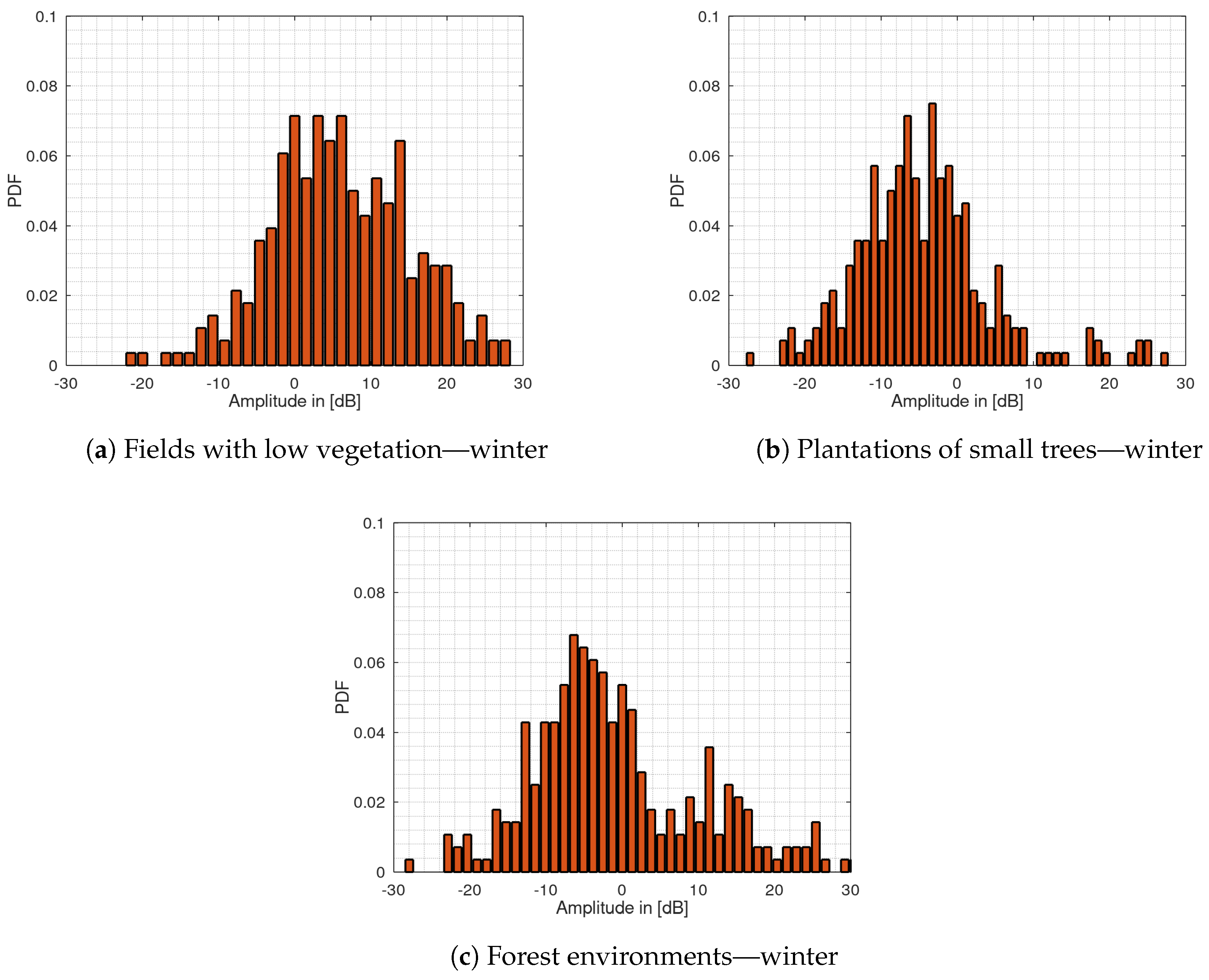
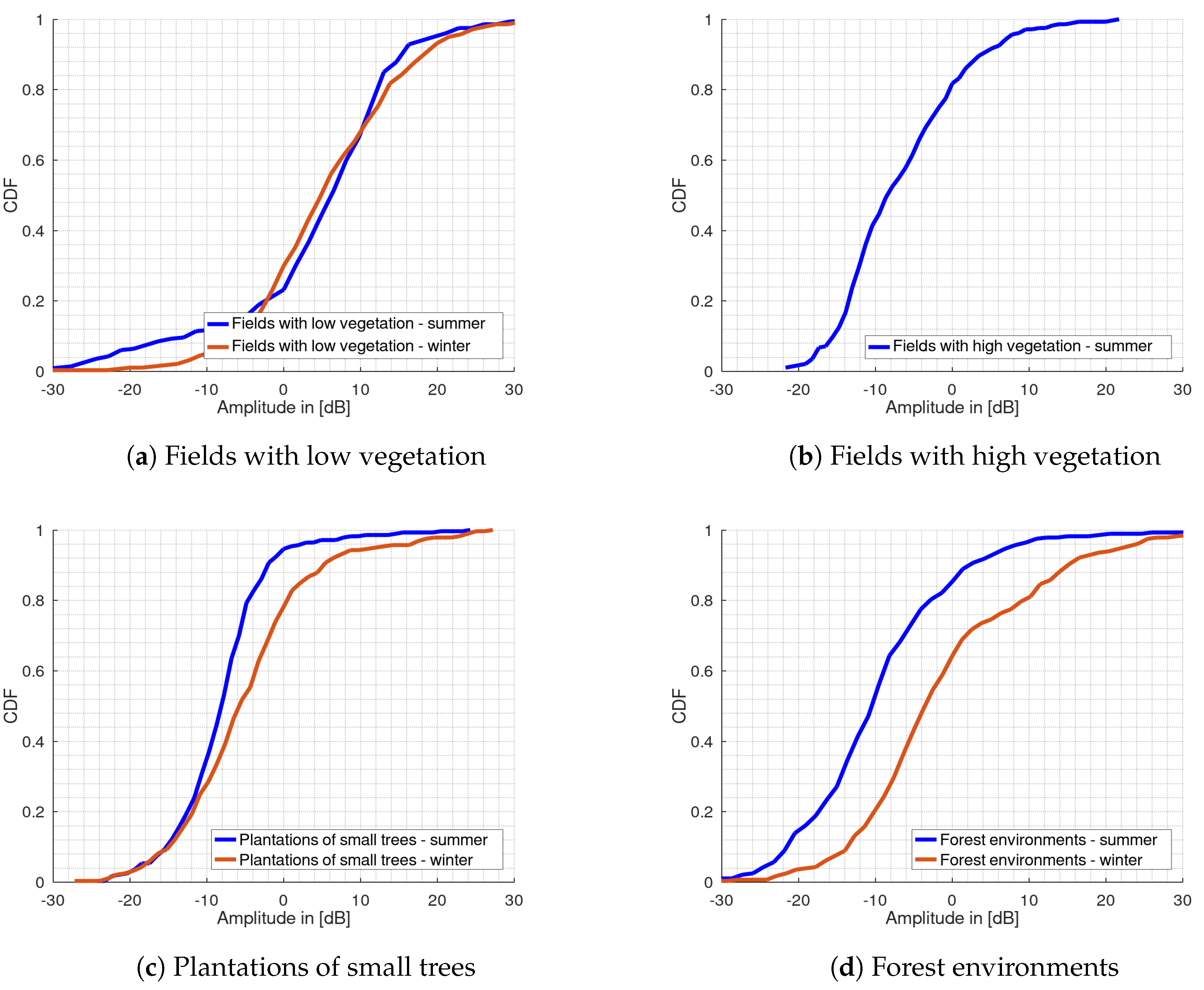
- Fields with low vegetation
- Fields with high vegetation
- Plantations with small trees
- Forest environments
2. Materials and Methods
2.1. Measurement Campaigns
2.2. The Bistatic Radar Setup
2.2.1. The Dual-Channel Bistatic Receiver
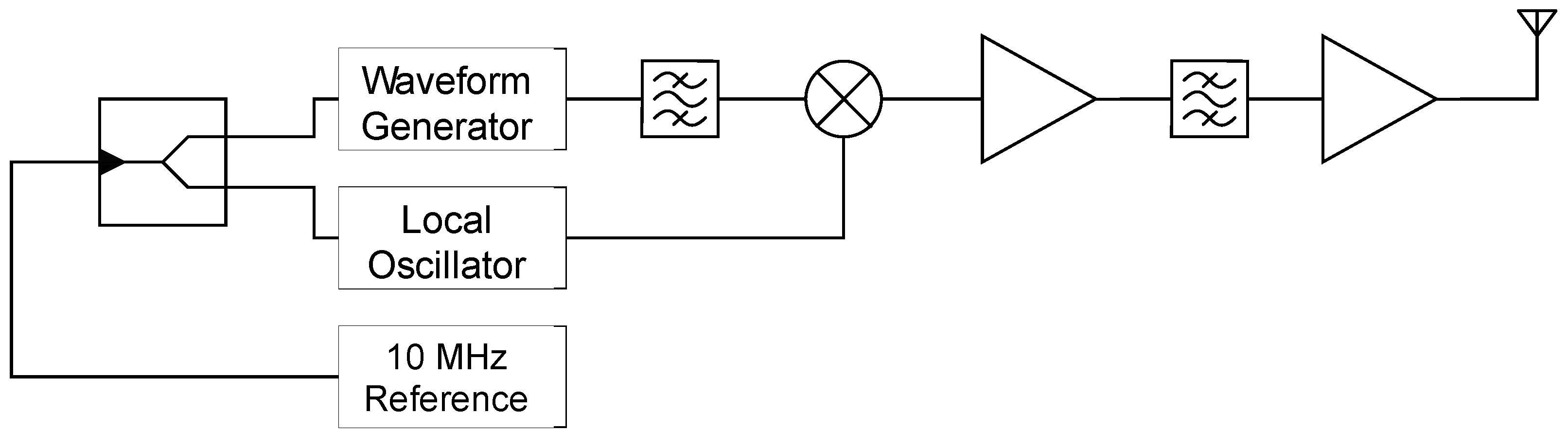
2.2.2. The X-Band Transmitter Used as Illuminator
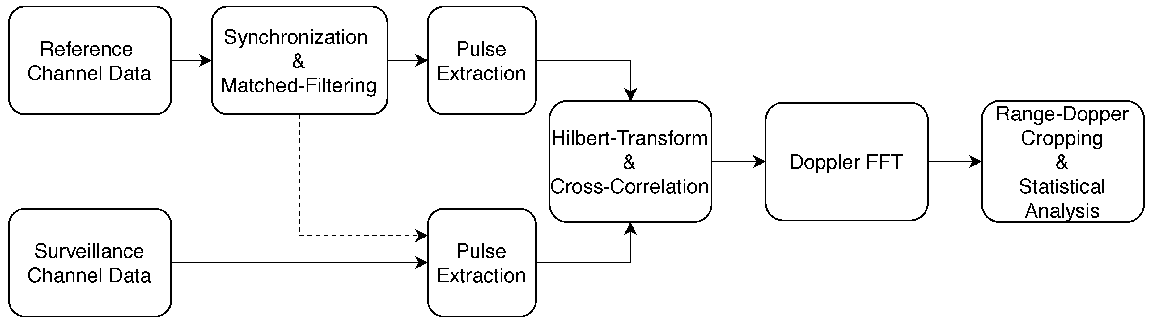
2.3. The Coherent Signal Processing Approach
2.4. Statistical Parameters
3. Results
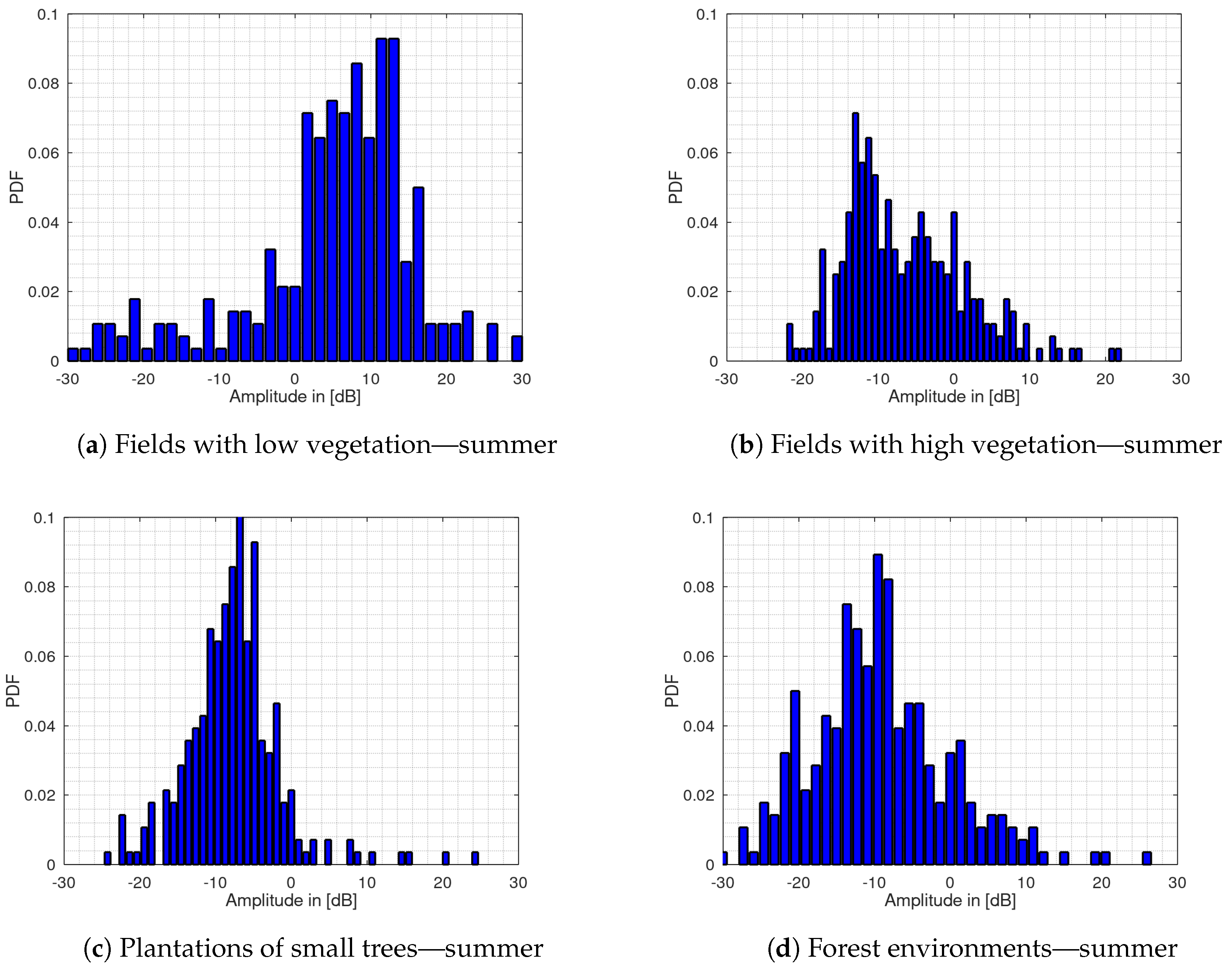
3.1. Histogram Plots
3.2. Clutter Cumulative Distribution Functions
3.3. Descriptive Clutter Statistics
4. Discussion
5. Conclusions
Author Contributions
Funding
Acknowledgments
Conflicts of Interest
Abbreviations
| PCL | Passive Coherent Location |
| SNIR | Signal-To-Interference-Plus-Noise Ratio |
| AWG | Arbitrary Waveform Generator |
| CPI | Coherent Processing Interval |
| FFT | Fast Fourier Transform |
| Probability Density Function | |
| PCC | Pearson Correlation Coefficient |
| CDF | Cumulative Distribution Function |
| IQR | Interquartile Range |
| CFAR | Constant False Alarm Rate |
| STAP | Space-Time Adaptive Processing |
References
- Willis, N.J.; Griffiths, H.D. Advances in Bistatic Radar; Institution of Engineering and Technology: London, UK, 2008. [Google Scholar]
- Griffiths, H.D. From a different perspective: Principles, practice and potential of bistatic radar. In Proceedings of the International Conference on Radar (IEEE Cat. No.03EX695), Adelaide, SA, Australia, 3–5 September 2003; pp. 1–7. [Google Scholar]
- Willis, N.J. Bistatic Radar; Institution of Engineering and Technology: London, UK, 2005. [Google Scholar]
- Colone, F.; O’hagan, D.W.; Lombardo, P.; Baker, C.J. A multistage processing algorithm for disturbance removal and target detection in passive bistatic radar. IEEE Trans. Aerosp. Electron. Syst. 2009, 45, 698–722. [Google Scholar] [CrossRef]
- Griffiths, H.D.; Baker, C.J. Passive coherent location radar systems. Part 1: Performance prediction. IEE Proc. Radar Sonar Navig. 2005, 152, 153–159. [Google Scholar] [CrossRef]
- Baker, C.J.; Griffiths, H.D.; Papoutsis, I. Passive coherent location radar systems. Part 2: Waveform properties. IEE Proc. Radar Sonar Navig. 2005, 152, 160–168. [Google Scholar] [CrossRef]
- Subotic, N.S.; Thelen, B.; Cooper, K.; Buller, W.; Parker, J.; Browning, J.; Beyer, H. Distributed RADAR waveform design based on compressive sensing considerations. In Proceedings of the 2008 IEEE Radar Conference, Rome, Italy, 26–30 May 2008; pp. 1–6. [Google Scholar]
- Cheng, X.; Aubry, A.; Ciuonzo, D.; De Maio, A.; Wang, X.S. Robust Waveform and Filter Bank Design of Polarimetric Radar. IEEE Trans. Aerosp. Electron. Syst. 2017, 53, 370–384. [Google Scholar] [CrossRef]
- Yang, Y.; Blum, R.S. MIMO radar waveform design based on mutual information and minimum mean-square error estimation. IEEE Trans. Aerosp. Electron. Syst. 2007, 43, 330–343. [Google Scholar] [CrossRef]
- Weiner, M.M.; Kaplan, P. Bistatic Surface Clutter Resolution Area at Small Grazing Angles; Technical report; Rome Air Development Center: Griffiss Air Force Base, NY, USA, 1982. [Google Scholar]
- Billingsley, J.B.; Farina, A.; Gini, F.; Greco, M.V.; Verrazzani, L. Statistical analyses of measured radar ground clutter data. IEEE Trans. Aerosp. Electron. Syst. 1999, 35, 579–593. [Google Scholar] [CrossRef]
- Billingsley, J.; Larrabee, J.F. Multifrequency Measurements of Radar Ground Clutter at 42 Sites. Volume 2. Appendices A through D; Technical report; Lincoln Laboratory: Lexington, MA, USA, 1991. [Google Scholar]
- Billingsley, J.B. Low-Angle Radar Land Clutter: Measurements and Empirical Models; Institution of Engineering and Technology: London, UK, 2002. [Google Scholar]
- Greco, M.; Gini, F.; Farina, A.; Billingsley, J.B. Validation of windblown radar ground clutter spectral shape. IEEE Trans. Aerosp. Electron. Syst. 2001, 37, 538–548. [Google Scholar] [CrossRef]
- Billingsley, J.; Larrabee, J. Measured spectral extent of L-and X-radar reflections from windblown trees. Proj. Rep. 1987. [Google Scholar] [CrossRef]
- Billingsley, J.B. Exponential Decay in Windblown Radar Ground Clutter Doppler Spectra: Multifrequency Measurements and Model; Technical report; Lincoln Laboratory: Lexington, MA, USA, 1996. [Google Scholar]
- Lombardo, P.; Billingsley, J.B. A new model for the Doppler spectrum of windblown radar ground clutter. In Proceedings of the 1999 IEEE Radar Conference. Radar into the Next Millennium (Cat. No.99CH36249), Waltham, MA, USA, 20–22 April 1999; pp. 142–147. [Google Scholar]
- Chen, K.S.; Fung, A.K. Frequency dependence of backscattered signals from forest components. IEE Proc. Radar Sonar Navig. 1995, 142, 301–305. [Google Scholar] [CrossRef]
- Jao, J. Amplitude distribution of composite terrain radar clutter and the K-Distribution. IEEE Trans. Antennas Propag. 1984, 32, 1049–1062. [Google Scholar]
- Billingsley, J.B. Radar Ground Clutter Measurements and Models. Part 1. Spatial Amplitude Statistics; Technical report; Lincoln Laboratory: Lexington, MA, USA, 1991. [Google Scholar]
- Chan, H. Spectral Characteristics of Llow-Angle Radar Ground Clutter; Technical report; Defence Research Establishment Ottawa: Ottawa, ON, Canada, 1989. [Google Scholar]
- Zhu, G.; Chen, Y.; Yin, H. Analiysis of typical ground clutter statistical characteristics. In Proceedings of the 2017 International Applied Computational Electromagnetics Society Symposium (ACES), Suzhou, China, 1–4 August 2017; pp. 1–2. [Google Scholar]
- Menon, K.R.; Balakrishnan, N.; Janahraman, M.; Ramchand, K. Characterization of fluctuation statistics of radar clutter for Indian terrain. IEEE Trans. Geosci. Remote Sens. 1995, 33, 317–324. [Google Scholar] [CrossRef]
- Ulaby, F.; Dobson, M.C.; Álvarez-Pérez, J.L. Handbook of Radar Scattering Statistics for Terrain; Artech House: Miami, FL, USA, 2019. [Google Scholar]
- Strydom, J.J.; de Witt, J.J.; Cilliers, J.E. High range resolution X-band urban radar clutter model for a DRFM-based hardware in the loop radar environment simulator. In Proceedings of the 2014 International Radar Conference, Lille, France, 13–17 October 2014; pp. 1–6. [Google Scholar]
- Melebari, A.; Gaffar, M.Y.A.; Strydom, J.J. Analysis of high resolution land clutter using an X-band radar. In Proceedings of the 2015 IEEE Radar Conference, Johannesburg, South Africa, 27–30 October 2015; pp. 139–144. [Google Scholar]
- Boothe, R.R. The Weibull Distribution Applied to the Ground Clutter Backscatter Coefficient; Technical report; Defense Technical Information Center: Redstone Arsenal, AL, USA, 1969. [Google Scholar]
- Schleher, D.C. Radar Detection in Weibull Clutter. IEEE Trans. Aerosp. Electron. Syst. 1976, AES-12, 736–743. [Google Scholar] [CrossRef]
- Melebari, A.; Mishra, A.K.; Abdul Gaffar, M.Y. Statistical analysis of measured high resolution land clutter at X-band and clutter simulation. In Proceedings of the 2015 European Radar Conference (EuRAD), Paris, France, 9–11 September 2015; pp. 105–108. [Google Scholar]
- Bundesamt, S. Bodenfläche Insgesamt Nach Nutzungsarten in Deutschland. 2020. Available online: https://www.destatis.de/DE/Themen/Branchen-Unternehmen/Landwirtschaft-Forstwirtschaft-Fischerei/Flaechennutzung/Tabellen/bodenflaeche-insgesamt.html (accessed on 17 May 2020).
- Für, E.; Landwirtschaft, B. Bodennutzung und Pflanzliche Erzeugung. 2020. Available online: https://www.destatis.de/DE/Themen/Branchen-Unternehmen/Landwirtschaft-Forstwirtschaft-Fischerei/Publikationen/Bodennutzung/bodennutzung-erzeugung-2030300147005.html (accessed on 17 May 2020).
- Für, E.; Landwirtschaft, B. Entwicklung der Gesamtfläche nach Nutzungsarten. 2020. Available online: https://www.bmel-statistik.de/landwirtschaft/ernte-und-qualitaet/bodennutzung/ (accessed on 17 May 2020).
- Kohler, M.; Weiss, M.; Saam, A.; Worms, J.; O’Hagan, D.W.; Bringmann, O. External Timebase Trials for Phase Coherency of a Bistatic Transfer Function Measurement Setup. In Proceedings of the 2019 Signal Processing Symposium (SPSympo), Krakow, Poland, 17–19 September 2019; pp. 319–322. [Google Scholar]
- Kohler, M.; Saam, A.; Worms, J.; O’Hagan, D.W.; Novacek, J.; Bringmann, O. Delay Estimation for Time Synchronization of a Bistatic Transfer Function Measurement Setup to Single Received Pulses. In Proceedings of the 2019 Signal Processing: Algorithms, Architectures, Arrangements, and Applications (SPA), Poznan, Poland, 18–20 September 2019; pp. 62–66. [Google Scholar]
- Duk, V.; Cristallini, D.; Wojaczek, P.; O’Hagan, D.W. Statistical Analysis of Clutter for Passive Radar on an Airborne Platform. In Proceedings of the 2019 International Radar Conference (RADAR), Toulon, France, 23–27 September 2019; pp. 1–6. [Google Scholar]
- Wang, Y.; Xia, W.; He, Z. CFAR Knowledge-Aided Radar Detection With Heterogeneous Samples. IEEE Signal Process Lett. 2017, 24, 693–697. [Google Scholar] [CrossRef]
- Wang, P.; Li, H.; Himed, B. A Bayesian Parametric Test for Multichannel Adaptive Signal Detection in Nonhomogeneous Environments. IEEE Signal Process Lett. 2010, 17, 351–354. [Google Scholar] [CrossRef]
- Ciuonzo, D.; Orlando, D.; Pallotta, L. On the Maximal Invariant Statistic for Adaptive Radar Detection in Partially Homogeneous Disturbance With Persymmetric Covariance. IEEE Signal Process Lett. 2016, 23, 1830–1834. [Google Scholar] [CrossRef]


| Terrain under Test | Fields with Low Vegetation Winter | Plantations of Small Trees Winter | Forest Environment Winter |
|---|---|---|---|
| Fields with low vegetation summer | 0.78 | 0.1 | 0.18 |
| Plantations of small trees summer | −0.16 | 0.76 | 0.59 |
| Forest environment summer | −0.04 | 0.84 | 0.64 |
| Terrain under Test | IQR | Skewness | Kurtosis | |
|---|---|---|---|---|
| Fields with low vegetation—summer | 11.8 dB | 10.8 dB | −0.98 | 1.7 |
| Fields with high vegetation—summer | 7.9 dB | 11.2 dB | 0.73 | 0.5 |
| Plantations of small trees—summer | 6.2 dB | 6.3 dB | 0.98 | 4.4 |
| Forest environment—summer | 10.0 dB | 11.1 dB | 0.88 | 2.3 |
| Fields with low vegetation—winter | 10.1 dB | 13.1 dB | −0.11 | 1.3 |
| Plantations of small trees—winter | 9.0 dB | 10.1 dB | 0.84 | 1.64 |
| Forest environment—winter | 11.7 dB | 14.4 dB | 0.62 | 0.33 |
© 2020 by the authors. Licensee MDPI, Basel, Switzerland. This article is an open access article distributed under the terms and conditions of the Creative Commons Attribution (CC BY) license (http://creativecommons.org/licenses/by/4.0/).
Share and Cite
Kohler, M.; O’Hagan, D.W.; Weiss, M.; Wegner, D.; Worms, J.; Bringmann, O. Statistical Analysis of Bistatic Radar Ground Clutter for Different German Rural Environments. Sensors 2020, 20, 3311. https://doi.org/10.3390/s20113311
Kohler M, O’Hagan DW, Weiss M, Wegner D, Worms J, Bringmann O. Statistical Analysis of Bistatic Radar Ground Clutter for Different German Rural Environments. Sensors. 2020; 20(11):3311. https://doi.org/10.3390/s20113311
Chicago/Turabian StyleKohler, Michael, Daniel W. O’Hagan, Matthias Weiss, David Wegner, Josef Worms, and Oliver Bringmann. 2020. "Statistical Analysis of Bistatic Radar Ground Clutter for Different German Rural Environments" Sensors 20, no. 11: 3311. https://doi.org/10.3390/s20113311
APA StyleKohler, M., O’Hagan, D. W., Weiss, M., Wegner, D., Worms, J., & Bringmann, O. (2020). Statistical Analysis of Bistatic Radar Ground Clutter for Different German Rural Environments. Sensors, 20(11), 3311. https://doi.org/10.3390/s20113311