Article

PortWeather: A Lightweight Onboard Solution for Real-Time Weather Prediction

1
Department of Informatics and Telecommunication, University of Ioannina, 45110 Ioannina, Greece
2
Department of Computer Science, University of Pisa, 56126 Pisa, Italy
3
Computer Technology & Press “Diophantus”, 26504 Patras, Greece
*
Author to whom correspondence should be addressed.
Sensors 2020, 20(11), 3181; https://doi.org/10.3390/s20113181
Submission received: 17 April 2020 / Revised: 29 May 2020 / Accepted: 30 May 2020 / Published: 3 June 2020

Abstract

:
Maritime journeys significantly depend on weather conditions, and so meteorology has always had a key role in maritime businesses. Nowadays, the new era of innovative machine learning approaches along with the availability of a wide range of sensors and microcontrollers creates increasing perspectives for providing on-board reliable short-range forecasting of main meteorological variables. The main goal of this study is to propose a lightweight on-board solution for real-time weather prediction. The system is composed of a commercial weather station integrated with an industrial IOT-edge data processing module that computes the wind direction and speed forecasts without the need of an Internet connection. A regression machine learning algorithm was chosen so as to require the smallest amount of resources (memory, CPU) and be able to run in a microcontroller. The algorithm has been designed and coded following specific conditions and specifications. The system has been tested on real weather data gathered from static weather stations and onboard during a test trip. The efficiency of the system has been proven through various error metrics.

1. Introduction

Meteorology is the study of weather events, having a significant focus on the forecasting of principal weather variables. Prediction on weather conditions is performed by using historical data or mathematical models [1] or a combination of both. There is great importance in quantifying meteorological variables such as temperature, humidity, air pressure, and wind flow; their variations and interactions and how they change over time. For this reason, various spatial scales have been proposed in order to describe and predict weather conditions on local, regional, or global levels [2,3].
Weather conditions have had a significant effect on sea-transportation and all the maritime affairs over time [4]. Maritime activities are related to maritime commerce and maritime leisure, but they also affect the environment and consequently atmosphere and so weather conditions. All are related and interconnected and seem to belong to a vicious circle that impact the quality of the environment and the maritime meteorological conditions [5,6]. The safety of maritime transportation is strictly related to weather information. International Maritime Organization (IMO) [7] and the World Meteorological Organization (WMO) [8] have proposed and defined regulation strategies on how to provide marine weather predictions to minimize accidents and economic losses.
For these reasons, as also reported in [4], there is an essential need for maritime weather prediction systems, which is connected to the sustainable development of sea commerce. The development of advanced, real-time and onboard forecast systems is becoming of significant importance in order to achieve high weather forecast quality (especially with regard to storms, heavy precipitation, wind, waves, and extreme temperatures).
In the era of Machine Learning (ML), there are available several methods that could be investigated, adapted, expanded and tested in order to be used for weather prediction. The main approaches for weather prediction could be classified in the following four categories [9]:
  • nowcast: which predicts the current wind speed;
  • short-term: where the weather parameters are predicted for the next 72 h [10];
  • medium-range: where the time scale increases to a period of 3–7 days and finally;
  • long-term: where the weather conditions are predicted for a period from one week to months or even years [11].
When it comes to forecasting meteorological parameters like wind speed and wind direction, special care must be taken in order to tackle the problem of the local environment and the complexity of these parameters [12,13] which can seriously affect the performance of the forecasting methods [14,15]. Hence, it is a common approach to test several machine learning techniques to solve the weather forecasting problem [16,17]. However, all these algorithms can be classified into two main categories: online and trained. Trained models are ML algorithms that require a data-heavy learning phase before being able to produce predictions. These models are typically well-performing, but their forecasts are strongly linked to the training-set, thus making them not usable in moving scenarios like onboard weather prediction. On the contrary, online learning models are algorithms that continuously learn and adapt their predictions capabilities to the flow of data. These algorithms are the best candidates for the development of an onboard weather prediction system for maritime applications because the vessel position change does not influence them.
Nowadays, the Internet of Things (IoT) initiative has allowed communication and interoperability between machines [18,19,20] and so, in the specific application area, meteorological data collection has become more accessible and performant [21,22,23]. The IoT is, in fact, one of the disruptive and essential technologies for fields such as meteorology, since it allows data from different machines to converge on servers through the use of various technologies such as wireless sensor networks (WSN) and Low Power Wide Area Network (LPWAN) [24]. Moreover, the increase in the computational capabilities of IoT devices enabled the local processing of data pushing the IoT toward the “edge” paradigm [25,26]. In the edge paradigm, sensors are also endowed with local processing capabilities, thus making them able to provide real-time analysis. In these scenarios, the connection with remote servers is used only for data storage and synchronization, making network stability and availability not necessary for the functioning of the system.
In the meteorological field, it is possible through the IoT-edge paradigm to develop low-cost solutions [27] both for the collection and display of data and for the forecasting based on machine learning algorithms executed directly on the IoT nodes. The junction of IoT and Artificial Intelligence has been named AIoT and is considered one of the most promising technologies for the development of innovative systems and services of the Industry 4.0 era [28].
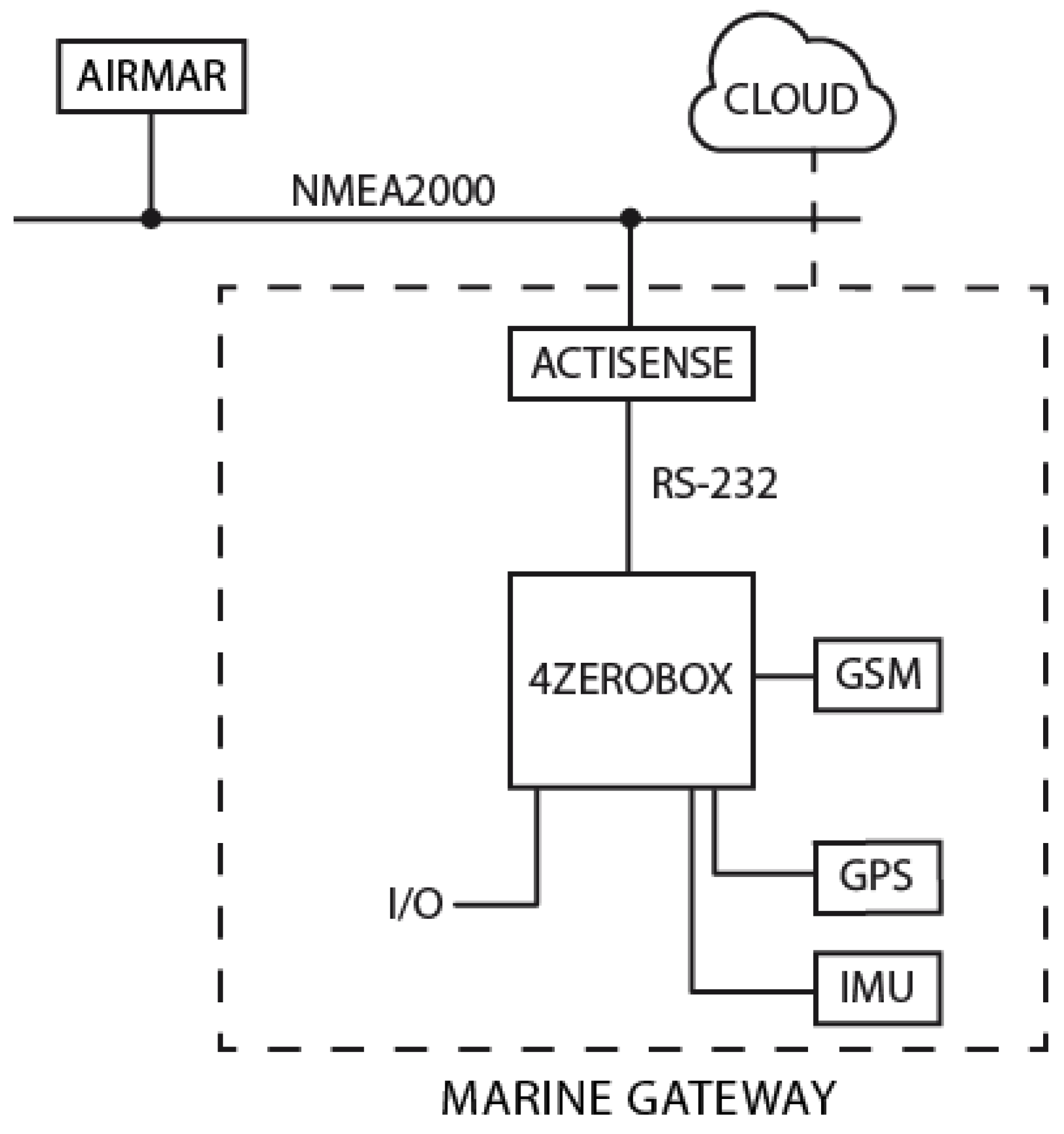
The goal of this work is to present a complete system named PortWeather, which forecasts the wind speed and direction at different horizons 30 min, 60 min, 90 min and two hours. The system consists of a commercial weather station which sends the current weather parameters to a local IOT unit based on a 32-bit micro-controller where the heart of the weather prediction algorithm runs without the need for a connection with a remote server.
The PortWeather system uses an online-learning ML weather forecast algorithm that does not require pre-train and the vessel position changes do not influence it. The system uses only local data to continuously train the weather predictor that produces the 30, 60, 90, and 120 min forecasts. Among various online learning algorithms developed for the weather forecast, a linear regression ML model has been chosen because it allows a lightweight implementation executable on a tiny microcontroller while still guaranteeing results comparable with more complex ML models.
Such integrated A-IoT edge solution has been designed for use on small professional and private boats that do not have the apparatus required for continuous connection to weather forecast remote services.
The PortWeather system has been tested on different datasets, including static data collected by ground weather stations and on a real sea trip where the system was installed on a test boat.
The PortWeather system can be easily installed on any typology of boats without requiring any training or ML/AI configuration. This feature makes the system easy to install, scalable, and also usable in long trips where the weather condition and micro-climate can change widely.
The manuscript is structured as follows: After the Introduction, Section 2 presents the state of the art in weather forecast systems and in ML algorithms currently used for weather prediction. Section 3 describes the PortWeather system, while Section 4 describes the preparation of the testing dataset and the results achieved by the forecast algorithm. Finally, Section 5 concludes the paper with some final remarks, recommendations, and suggestions for future work.

2. Related Works

2.1. Embedded Weather Forecasting Systems

Various weather station with forecasting capabilities are nowadays available on the market or have been developed as research activities. In [29], an Arduino based weather station is presented. The system collects data from various weather sensors processing them using a neural network. The network produces a “dressing index” that suggests to the users what would be the outdoor perceived temperature.
In [30,31], the creation of an embedded system for short-term weather forecast is presented. Like in the case of PortWeather, this system uses a tiny (PIC16F877) microcontroller as a computational unit. In this case, the forecast of meteorological variables (wind speed and direction, temperature, and relative humidity) is based on the juxtaposition of the data using five methods: Persistence Method, Trends Method, Climatology Method, Analog Method, and Numerical Weather Prediction Method. In this work, no machine learning method has been used, and no comparison to real data has been shown, making the system difficult to be compared with PortWeather or any other similar solution.
In [32], a low-power distributed IoT system has been developed for the prediction fo crop frost. The system is based on a network of weather parameters sensors connected through a Low Power Wide Area Network (LPWAN). In this work, all the sensors stream data to a central server that integrates them with data provided by public weather forecast services providing farmers and index of frost risk. Also in this case, the nodes use a microcontroller board, but no computation and processing of data are performed on-edge.
In [33], an interesting approach aimed at integrating Deep Learning (DL) weather forecast algorithms with IoT is presented. The system is composed of a series of data gathering node connected to a central server where the DL algorithm runs.
Most of the IOT and A-IOT (AI + IOT) systems for weather forecast have been designed as networks of sensors connected to a central server where all the AI/ML algorithms are executed. Moreover, most of these systems are based on ML algorithms that require data-intensive and difficult training phase.
To our knowledge, a system able to provide real-time local weather forecast using training-less ML algorithms executed on low-power, low-cost IOT units without the need of a continuous internet connection is still missing.

2.2. Machine Learning for Weather Prediction

A number of Machine Learning models have been already employed for the forecasting of different weather parameters. State-of-the-art techniques implemented successfully in this area include Artificial Neural Networks [34], Deep Learning techniques [35], Recursive Neural Networks [36], and Support Vector Machines [37]. On the other hand, there is a growing trend of combining various models or even ensemble methods [38].
All of these methods focus on batch learning where a ’batch’ of training data is provided, and the goal is to train the model that yields minimum error on predicting values. A significant disadvantage of these methods and their corresponding application is that they require big training dataset and enough memory to host them.
In [39], a performance analysis of time series forecasting models for short term wind speed prediction is presented. In this work, authors used a wind measurement station to collect: wind speed and direction, temperatures, humidity, and barometric pressure sensors. Six forecast algorithms have been tested: Random walk, Linear trend, Quadratic trend, Simple moving average, autoregressive moving average (ARIMA), and Nonlinear Autoregressive with an External Input (NARX) neural network model. The paper reports that the ARIMA and NARX models appear more successful than others demonstrating that regressive methods can be used for short time wind speed prediction.
In [40], another comparison of various algorithms for short-term weather prediction is reported. Authors highlight that online learning models such as Exponentially Weighted Moving Average (EWMA) and Simple Prior Moving Average (SPMA) perform better than static pre-trained neural networks while also allowing for avoiding the need of a training dataset for the priming of the model.
Indeed, there are specific types of machine learning processes where the model updates its parameters in a sequence of consecutive rounds. In these methods, there is no separation between the training phase and the testing phase, but the goal is to update the prediction model at the end of each trial to minimize the total loss over a sequence of trials [41]. Such type of learning process is called online learning [42] and arise in a variety of real-world applications, including prediction problems (e.g., forecasting the weather the next day) and decision/allocation problems (e.g., investing in different stocks or mutual funds) [43].
All these works highlight that online learning based prediction models are performing well in weather time series analysis and forecasting. Considering that they do not require a training phase and that are typically based on linear calculus, these models are good candidates for the development of server-free weather forecast IOT solutions.
In particular, linear regression models can be considered as an evolution of the Moving Average algorithm that allow a different weight for each parameter instead of the equal weight of each parameter in the case of the MA method. Moreover, Linear Regression allows a simple and lightweight implementation. For this reason, the PortWeather system prediction algorithm has been based on a linear regression model

3. The PortWeather System

Considering the complexity of performing weather forecasting on a boat without requiring an internet connection and algorithm pre-training, we decided to build a novel A-IOT system for sensor-driven real-time onboard weather prediction. The system is composed of: the weather station, which carries out continuous measurements of weather parameter and it is installed on the boat cabin roof; the data acquisition and elaboration unit and the machine learning algorithm that runs on the microcontroller of the data acquisition unit providing real-time weather predictions.

3.1. Hardware

The hardware involved in the construction of the system consists of two main parts: a weather station and the data acquisition and elaboration unit (called “Marine Gateway”). An architectural diagram of the PortWeather system is illustrated in Figure 1.

3.1.1. Weather Station

We installed a weather station (Airmar 220WX, Airmar Technology) on a tugboat unit. The Airmar station collects wind apparent speed and direction and, thanks to the availability of an integrated GPS and compass system, also calculates the real speed and direction of wind compensating the boat movement. Moreover, the data obtained from the GPS module are also used by the system for data and events chrono-referencing.
The weather station sends the data to the Marine Gateway using the NMEA 2000 protocol [44]. NMEA2000 is a widely used software protocol for maritime electronics that uses the CAN (Controller Area Network) as a transport protocol.
Table 1 reports technical details and features of the Airmar 220 weather station.
The weather station allows us to acquire a considerable amount of meteorological information in real time, through an all-in-one sensor system. Table 2 presents the data that the weather station gathers and provides:

3.1.2. Marine Gateway

The Marine Gateway is the acquisition and elaboration unit of the PortWeather system. The unit acquires data from the weather station via NMEA2000 and elaborates them using the integrated regression algorithm. All the computation, analysis, and forecasting is performed locally on the Marine Gateway using the integrated 32-bit microcontroller. If a GSM internet connection is available, data are also sent to the cloud [45], allowing further data analysis and visualization.
In order to interface the Marine Gateway with the Airmar weather station, an Actisense NMEA2000 to RS-232 protocol converter has been used.
The Marine Gateway core is an industrial-grade development board called 4ZeroBox. The 4ZeroBox (displayed in the Figure 2) is a modular hardware electronic unit that simplifies the development of Industrial IoT applications [19] allowing rapid and seamless interfacing with industrial sensors, actuators, and Cloud services [46].
The 4ZeroBox computational unit is based on the powerful 32-bit ESP32 microcontroller made by Espressif Systems (Shangai, China) (240 MHz, 4 Mb Flash, 512 KB SRAM). The 4zerobox is programmable in Python (or hybrid C/Python) thanks to the Zerynth software (v. 2.5.2, Zerynth, Pisa, Italy) [20,47].
The 4zerobox allows acquiring data from both digital and analog ports, thus making it possible to interface with digital connection enabled machines and apparatus (like in the case of the Airmar station) but also with auxiliary analog external sensors [24,48].
The 4ZeroBox supports Wi-fi, Bluetooth, Ethernet, LoRa (a modulation technique that guarantees long-range communications), RS485, and RS232 connection while also integrating an SD Card for local data storage. Moreover, the system also integrates two onboard MikroBUS sockets to extend the 4ZeroBox with hundreds of other sensors available as MikroElektronika click boards.
In the PortWeather configuration, the two MikroBus expansion sockets have been used for the GSM 3G modem and an IMU (Inertial Measurement Unit) sensor.
When the GSM connection is available, data stored temporarily on the SD card are transferred to the Zerynth Device [49] services using the MQTT (Message Queuing Telemetry Transport) protocol.
Table 3 presents the technical description of the 4ZeroBox.
Technical specification of the ESP32 microcontroller at the core of the 4ZeroBox is reported in Table 4.

3.2. Software

In the designing and the development of the PortWeather system, the problems of high overhead, low efficiency, and low speed were addressed. A small memory footprint Machine Learning algorithm was selected, developed, and implemented using a regression method allowing the execution on a low memory microcontroller.

3.2.1. Zerynth Platform

There are various hardware abstraction layer libraries, RTOSs, and interpreted language engines for the programming of microcontroller available on the market. However, considering the need for developing a Machine Learning model for weather prediction, we preferred to focus toward a complete and reliable developing framework able to support Python and, in particular, hybrid C/Python coding. For this reason, Zerynth [47] has been selected as the developing framework for the PortWeather project.
Zerynth [20] is a software suite composed of several tools that allow programming of 32-bit microcontrollers in Python or hybrid C/Python by also allowing a seamless connection of the implemented devices to various cloud platforms. Zerynth includes a compiler, debugger, and an editor, alongside various tutorials and example projects for a smooth learning experience. Moreover, Zerynth is natively supported by the 4ZeroBox, together with all various libraries necessary for the management of integrated peripherals, protocols, and sensors.

3.2.2. Regression Methods

Regression is a type of problem that aims at predicting an output from a number of inputs using a limited number of data. Here, we use the following notation, x R m , which describes the input features, and y i denotes the target/output value of a parameter like the wind speed (or the wind direction) that we need to forecast. Thus, { x i , y i } in our case will be training data and the list of training data is often called dataset. The dataset consists of a number n of training data { x i , y i | i = 1 , . . . , n } . R n · m denotes the input space, and R n the output space of n values. Regression is our basic problem since the target parameters y i (wind speed and direction) are continuous.
Thus, the whole problem is simply reduced to find a function like X n · m Y n · 1 , for which we minimize the error between the real wind speed value and the predicted wind speed value. In this study, the available features are Temperature, Humidity, Wind direction and speed, and Barometric Pressure, while the value to predict are the wind speed direction. We also keep a record of the previous four values of each parameter which are fed as input to the regression model. One of the simpler algorithms that can be used for this purpose is Linear Regression (LR), which, in our case, seeks to predict the wind speed and direction as a linear combination of the input features.
In order to approximate y (wind speed and direction) as a linear functions of x i :
h θ ( x ) = θ 0 + θ 1 x 1 + . . . + θ m x m = i = 1 m θ i x i
where x 0 = 1 and θ = { θ i | i = 1 , . . . , m } are the parameters of the linear function mapping from X n · m to Y n · 1 .
The common error function used to calculate the difference between the output h θ ( x ) and the actual value y i is the least square error function defined in terms of:
J ( θ ) = 1 2 i = 1 n ( h θ ( x i ) y i ) 2
For the minimization of the error J ( θ ) , a successful approach would be the Gradient Descent method which changes the values of the parameters repeatedly until convergence to a minimum value. The Gradient Descent method can be described as the following update on the parameters θ :
θ j n e w = θ j o l d a J ( θ ) θ j
where a is the learning rate that is usually set to 10 3 a 10 2 and smaller values for the learning rate leads to slower convergence.
However, in the case of microcontrollers, the Central Processing Unit (CPU) clock frequency is very low, and the memory is minimal. Thus, the machine-learning algorithm must be designed in order to tackle both of these problems. On the other hand, Stochastic Gradient Descent (SGD) [50] is an iterative procedure which has successfully used to optimize a function. The main advance of this SGD learning algorithm is that the parameters of the model are updated as the new data arrive [51]. This kind of procedure is currently gaining interest in the Deep Learning community [52].
In the case of the SGD algorithm, the update on the parameters is performed for a pair ( x i . y i ) from the training set as:
θ j n e w = θ j o l d a J ( θ ; x i . y i ) θ j
In SGD, the learning rate a is typically much smaller than any corresponding learning rate in Batch Gradient Descent algorithm because there is much more variance in the update.
In this work, the SGD algorithm was implemented through the use of a Flash Matrix table in which the acquired measurements are stored. The matrix is filled in a round-robin way so that those older measurements are eliminated in favor of more recent measurements.
The system has no pre-trained model saved. When the system boots, the first data are used for the learning of the algorithm; thus, the predictor does not produce any output. The method has only a short-term training memory, so it continuously adapts to current inputs making the system usable in any weather condition and geographical location. If the system is shut down for an extended period or if the sensors are changed, the system is thus able to adapt to the new conditions without requiring re-training.
However, all these conditions are infrequent in the maritime context where boats are used in limited geographical areas, and equipment change is due only to maintenance interventions.
Finally, the use of a low-power microcontroller-based data acquisition unit allows leaving the system always on also when the boat is harboured. This allows the PortWeather system to learn continuously being always ready for use.

4. PortWeather System Performance Tests

In order to test the prediction algorithm developed (both for the prediction of wind speed and wind direction), two main types of tests were performed: a static test and a dynamic test. In both cases, the results obtained for the predictions at 30, 60, 90, and 120 min were analyzed by calculating Median Absolute Error (MAE) and the Root Mean Square Error (RMSE), which are common measures for time series regression problems [53,54] and the mean absolute percentage error (MAPE) [55].
The measures are defined as:
M A E = 1 N i = 1 N y ^ i y i
R M S E = 1 N i = 1 N ( y ^ i y i ) 2
M A P E = 1 N i = 1 N | y ^ i y i y i |
where N is the number of the testing samples, y ^ i is the predicted value, and y i the true wind speed (or direction) value. However, RMSE may not be a good indicator of the average performance of the model [56]. Therefore, more importance will be given to the results obtained by the MAE.
We also calculated residual errors in the results of the predictions. The calculation of residual errors is realized as the difference between the predicted value y ^ i and the true wind speed (or direction) value y i , and it is carried out in order to have further confirmation of the validity of the model.

4.1. Land Weather Station Test

The static test was carried out for the preliminary checks of the algorithm developed. In this case, the data on which the algorithm was executed was acquired by static/land weather stations. The data were collected from 6 November 2019 00:00:00 to 10 November 2019 13:45:00 from the weather stations of Livorno and Pianosa, [57].
Figure 3 displays the locations of the weather stations:
Table 5 and Table 6 provide a brief description of the data acquired from the land weather stations of Livorno and Pianosa, respectively.
Figure 4 and Figure 5 present the comparisons between the real values and the respective forecasts for the Livorno weather station dataset (both for wind speed and direction).
Table 7 presents the main results showing the wind speed error rates for the Livorno weather station. In particular, in this case, it is noted that the prediction of the wind speed realized by the algorithm differs by at most ±1.3 m/s, in the case of forecasts at two hours, with respect to the real speed.
The calculated errors have been gathered, record by record, and Table 8 presents the distribution of the residual values for the Livorno Weather station data set. It is concluded that the results obtained are consistent with what is reported in the calculation of the MAE, in fact, in the worst case, which is the 2-h prediction, most residual values belong to the range [−2, 2].
In the case of Livorno’s wind direction prediction, the algorithms differs by at most ±17.91°, in the case of forecasts at 2 h, as described in the following Table 9.
Table 10 presents calculation of the errors for the wind direction for the Livorno station, with the distribution of the residual values. It is inferred that the results obtained are consistent with what is reported in the calculation of the MAE, in fact, in the worst case, the 2-h prediction, most residual values belong to the range [−18; +18].
Figure 6 and Figure 7 present the comparisons between the real values and the respective forecasts for the Pianosa weather station dataset (correspondingly for wind speed and direction).
Table 11 presents the error rates for wind speed prediction for the Pianosa weather station. In this case, the prediction of the wind speed realized by the algorithm differs by at most ±1.7 m/s, in the case of forecasts at 2 h, with respect to the real wind speed.
The calculated errors have been gathered recorded by record, and Table 12 presents the distribution of the residual values for the Pianosa weather station. It is conducted that the results obtained are consistent with what is reported in the calculation of the MAE, in fact, in the worst case, the 2-h prediction, most residual values belong to the range [−2; +2]:
The worse prediction of the wind direction realized by the algorithm differs from the real direction by at most ±22.75 , in the case of forecasts at two hours for the Pianosa weather station as one can see in Table 13.
Table 14 presents the error distribution for the wind direction parameter for the Pianosa weather station. It can be observed that the results obtained are consistent with what is reported in the calculation of the MAE, in fact, in the worst case, the 2-h prediction, most residual values belong to the range [−25; +25].
Both from the analysis of the errors and the study of the graphs, it is concluded that the implemented algorithm reaches a high accuracy in predicting the wind speed and direction using statically collected data.

4.2. Dynamic Test

After evaluating the accuracy of the prediction algorithm on statically collected data, we tested the algorithm on dynamic data acquired using the PortWeather system installed on a tugboat. For the test, the tugboat made a trip from Chios island (Greece) to Athens (Greece), and the data collection lasted from 22 January 2018 11:24:00 to 9 February 2018 12:50:00. Figure 8 displays the planned trip of the ship.
Table 15 provides a brief description of the data acquired from the on-board weather station.
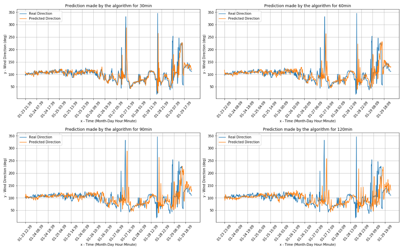
Figure 9 and Figure 10 present the comparisons between the real values and the respective forecasts (correspondingly for the wind speed and direction) for the onboard data set.
Table 16 presents the results showing the error rates for the onboard weather station. It is noted that the prediction of the wind speed realized by the algorithm differs by at most ±1.9 m/s, in the case of forecasts for 2-h prediction, with respect to the real wind speed.
The calculated errors have been recorded record by record, and Table 17 describes the distribution of the residual values. It is seen that the results obtained are consistent with what is reported in the calculation of the MAE, in fact, in the worst case, which is the 2-h prediction, most residual values belong to the range [−2; +2].
The worse prediction of the wind direction realized by the algorithm differs by at most ±20.3 , in the case of forecasts at 2 h, with respect to the real Wind direction as it can be seen in Table 18.
From the calculation of the errors, record by record, we have obtained Table 19 that describes the distribution of the residual values. The results obtained are consistent with what is reported in the calculation of the MAE, in fact, in the worst case, the 2-h prediction, most residual values belong to the range [−21; +21]:

4.3. Overall Evaluation

Table 20 and Table 21 present the MAE, MAPE, and RMSE error measures for the three different weather stations (Livorno, Pianosa and onboard) for the wind speed and wind direction, respectively. It can be inferred that, in terms of the MAE measure, the best accuracy of our method is performed for the Livorno data set for the wind speed and wind direction parameter. An increase of all the error measures is clearly reported with the increase of the prediction interval from 30 to 120 min.
The comparison of real and predicted value shows a time lag effect on the predicted data. As reported in [58], this effect is typical of simplified models where the prediction is highly correlated with a linear combination of historical data. However, although this effect is present, its visual analysis could lead to a misleading interpretation of the algorithm performances. Indeed, error measures analysis shows that the PortWeather system has relative low MAE, MAPE, and RMSE suggesting that the algorithm has an accuracy that is perfectly compatible with the kind of uses expected for the system.

5. Conclusions

This study presents an onboard weather prediction IOT system that provides short-term forecasts of wind speed and direction, without the need of an internet connection. The PortWeather system is composed of a commercial weather station interfaced with an Industrial IOT acquisition unit. The system is designed to be easy to install, reliable, and low-power, allowing the use on little and medium-sized boats. A forecasting algorithm based on linear regression was designed and implemented in order to work on a resource-constrained microcontroller for IOT applications. The implemented algorithm uses an online learning strategy allowing the system to work without the need of a training phase and Internet connection. This training-less approach allows the system to be resilient to boat geographical location shift and to recover from prolonged shutdown or sensors replacement quickly.
The efficiency of the system has been proven by testing the system in real sea conditions where weather parameters have been recorded on a tugboat operating in Greece. The algorithm performances have also been evaluated using other datasets, acquired from land weather stations located in different geographical and micro-climatic areas (Livorno and Pianosa, Italy).
As a general evaluation of the system, it is essential to highlight that linear regression algorithms are straightforward methods for the forecast of a time series evolution. These model are very simple, and sometimes it is possible to guess the output of these algorithms by looking at the time series plots. However, this is true for scientists but not for fishers and sea operators.
Maritime traffic security for little and medium-sized boats is an open challenge that needs to be addressed with accessible, scalable, and easy install and use solutions. Despite being based on an algorithm whose performances could be overcome nowadays by more complicated and computational massive neural-network-based algorithms, PortWeather can be considered as a reliable and innovative IOT solution for the real-time weather forecast on little and medium-size boats.
Although the system performs relatively well, there is room for improvement. We plan to install and test new microcontrollers that offer more CPU power as more memory. This will allow us to implement more advanced machine learning algorithms that could help in mitigating the time-lag effect introduced by the simplified regressive algorithm used in PortWeather. On the algorithm performance evaluation, it would be of extreme interest to evaluate the system in heavy weather conditions where the wind direction and speed parameter range are very high. Moreover, we plan to work on the system cloud connection going beyond the pure remote data storage for further analysis. On this side, it could be of extreme interest to allow the system to download historical weather data from publicly available Application Programming Interfaces (APIs) like Weather Underground [59] so that the system will be able to start instantly without the need for the initial training that is actually required at the boot.

Author Contributions

Conceptualization: P.K.; Methodology: P.K. and D.M.; Software: P.K. and M.B.; Hardware: D.M.; Validation: P.K., D.M. and M.B.; Data Curation: P.K., D.M., M.B. and C.S.; Writing—Original Draft Preparation: P.K., M.B., D.M.; Writing—Review & Editing: P.K., D.M., M.B. and C.S.; Funding Acquisition: D.M. and C.S. All authors have read and agreed to the published version of the manuscript.

Funding

This study is supported by “LINCOLN” (Lean Innovative Connected Vessels) Project (www.lincolnproject.eu) funded by Horizon 2020 research and innovation program (Grant Agreement: 727982) and co-funded by project: “Enhancing research activities of Laboratory of Knowledge and Intelligent Computing”, supported by the Research Committee of the University of Ioannina.

Conflicts of Interest

The authors declare no conflict of interest.

References

  1. Stensrud, D.J. Parameterization Schemes: Keys to Understanding Numerical Weather Prediction Models; Cambridge University Press: Cambridge, UK, 2009. [Google Scholar]
  2. Neumann, P.; Düben, P.; Adamidis, P.; Bauer, P.; Brück, M.; Kornblueh, L.; Klocke, D.; Stevens, B.; Wedi, N.; Biercamp, J. Assessing the scales in numerical weather and climate predictions: Will exascale be the rescue? Philos. Trans. R. Soc. A 2019, 377, 20180148. [Google Scholar] [CrossRef]
  3. Kalnay, E.; Kanamitsu, M.; Baker, W. Global numerical weather prediction at the National Meteorological Center. Bull. Am. Meteorol. Soc. 1990, 71, 1410–1428. [Google Scholar] [CrossRef]
  4. Wu, Y.; Pelot, R.P.; Hilliard, C. The influence of weather conditions on the relative incident rate of fishing vessels. Risk Anal. Int. J. 2009, 29, 985–999. [Google Scholar] [CrossRef] [PubMed]
  5. Kolios, S.; Vorobev, A.V.; Vorobeva, G.R.; Stylios, C. GIS and Environmental Monitoring: Applications in the Marine, Atmospheric and Geomagnetic Fields; Springer: Berlin/Heidelberg, Germany, 2017; Volume 20. [Google Scholar]
  6. Dinwoodie, J.; Tuck, S.; Knowles, H.; Benhin, J.; Sansom, M. Sustainable development of maritime operations in ports. Bus. Strategy Environ. 2012, 21, 111–126. [Google Scholar] [CrossRef]
  7. Wieslaw, T. Origins of ship safety requirements formulated by International Maritime Organization. Procedia Eng. 2012, 45, 847–856. [Google Scholar] [CrossRef] [Green Version]
  8. McMichael, A.J.; Haines, A.; Slooff, R. Climate change and human health: An assessment prepared by a task group on behalf of the World Health Organization, the World Meteorological Organization and the United Nations Environment Programme. In Climate Change and Human Health: An Assessment Prepared by a Task Group on Behalf of the World Health Organization, the World Meteorological Organization and the United Nations Environment Programme; OMS: Geneva, Switzerland, 1996. [Google Scholar]
  9. Bauer, P.; Thorpe, A.; Brunet, G. The quiet revolution of numerical weather prediction. Nature 2015, 525, 47. [Google Scholar] [CrossRef] [PubMed]
  10. Brewster, K.; Hu, M.; Xue, M.; Gao, J. Efficient assimilation of radar data at high resolution for short-range numerical weather prediction. In Proceedings of the World Weather Research Program Symposium on Nowcasting and Very Short-Range Forecasting, WSN05, Tolouse, France, 5–9 September 2005; Volume 3. [Google Scholar]
  11. Elliott, R.D. Extended-range forecasting by weather types. In Compendium of Meteorology; Springer: Berlin/Heidelberg, Germany, 1951; pp. 834–840. [Google Scholar]
  12. McInnes, K.L.; Erwin, T.A.; Bathols, J.M. Global Climate Model projected changes in 10 m wind speed and direction due to anthropogenic climate change. Atmos. Sci. Lett. 2011, 12, 325–333. [Google Scholar] [CrossRef]
  13. Katz, R.W.; Brown, B.G. Extreme events in a changing climate: Variability is more important than averages. Clim. Chang. 1992, 21, 289–302. [Google Scholar] [CrossRef]
  14. Allen, M.R.; Stott, P.A.; Mitchell, J.F.; Schnur, R.; Delworth, T.L. Quantifying the uncertainty in forecasts of anthropogenic climate change. Nature 2000, 407, 617. [Google Scholar] [CrossRef]
  15. Giorgi, F. Climate change prediction. Clim. Chang. 2005, 73, 239–265. [Google Scholar] [CrossRef]
  16. Karvelis, P.; Kolios, S.; Georgoulas, G.; Stylios, C. Ensemble learning for forecasting main meteorological parameters. In Proceedings of the 2017 IEEE International Conference on Systems, Man, and Cybernetics (SMC), Banff, AB, Canada, 5–8 October 2017; pp. 3711–3714. [Google Scholar]
  17. Georgoulas, G.; Kolios, S.; Karvelis, P.; Stylios, C. Examining nominal and ordinal classifiers for forecasting wind speed. In Proceedings of the 2016 IEEE 8th International Conference on Intelligent Systems (IS), Sofia, Bulgaria, 4–6 September 2016; pp. 504–509. [Google Scholar]
  18. Farooq, M.U.; Waseem, M.; Mazhar, S.; Khairi, A.; Kamal, T. A review on internet of things (IoT). Int. J. Comput. Appl. 2015, 113, 1–7. [Google Scholar]
  19. Mazzei, D.; Baldi, G.; Fantoni, G.; Montelisciani, G.; Pitasi, A.; Ricci, L.; Rizzello, L. A Blockchain Tokenizer for Industrial IOT trustless applications. Future Gener. Comput. Syst. 2020, 105, 432–445. [Google Scholar] [CrossRef]
  20. Mazzei, D.; Baldi, G.; Montelisciani, G.; Fantoni, G. A full stack for quick prototyping of IoT solutions. Ann. Telecommun. 2018, 73, 439–449. [Google Scholar] [CrossRef]
  21. Karvelis, P.; Michail, T.; Mazzei, D.; Petsios, S.; Bau, A.; Montelisciani, G.; Stylios, C. Adopting and Embedding Machine Learning Algorithms in Microcontroller for Weather Prediction. In Proceedings of the 2018 International Conference on Intelligent Systems (IS), Funchal, Portugal, 25–27 September 2018; pp. 474–478. [Google Scholar]
  22. Eleftheriou, A.; Kouvaris, K.; Karvelis, P.; Stylios, C. Micro Climate Prediction Utilising Machine Learning Approaches. In Proceedings of the 2018 IEEE International Workshop on Metrology for the Sea; Learning to Measure Sea Health Parameters (MetroSea), Bari, Italy, 8–10 October 2018; pp. 197–200. [Google Scholar]
  23. Karvelis, P.; Petsios, S.; Georgoulas, G.; Stylios, C. Short Time Wind Forecasting with Uncertainty. In Proceedings of the 2019 10th International Conference on Information, Intelligence, Systems and Applications (IISA), Patras, Greece, 15–17 July 2019. [Google Scholar]
  24. Gubbi, J.; Buyya, R.; Marusic, S.; Palaniswami, M. Internet of Things (IoT): A vision, architectural elements, and future directions. Future Gener. Comput. Syst. 2013, 29, 1645–1660. [Google Scholar] [CrossRef] [Green Version]
  25. El-Sayed, H.; Sankar, S.; Prasad, M.; Puthal, D.; Gupta, A.; Mohanty, M.; Lin, C.T. Edge of things: The big picture on the integration of edge, IoT and the cloud in a distributed computing environment. IEEE Access 2017, 6, 1706–1717. [Google Scholar] [CrossRef]
  26. Li, H.; Ota, K.; Dong, M. Learning IoT in edge: Deep learning for the Internet of Things with edge computing. IEEE Netw. 2018, 32, 96–101. [Google Scholar] [CrossRef] [Green Version]
  27. Kulkarni, A.; Mukhopadhyay, D. Internet of things based weather forecast monitoring system. Indones. J. Electr. Eng. Comput. Sci. 2018, 9, 555–557. [Google Scholar] [CrossRef]
  28. Vermesan, O.; Bröring, A.; Tragos, E.; Serrano, M.; Bacciu, D.; Chessa, S.; Gallicchio, C.; Micheli, A.; Dragone, M.; Saffiotti, A.; et al. Internet of Robotic Things: Converging Sensing/Actuating, Hypoconnectivity, Artificial Intelligence and IoT Platforms. In Cognitive Hyperconnected Digital Transformation: Internet of Things Intelligence Evolution; River Publishers: Copenhagen, Denmark, 2017; pp. 97–155. [Google Scholar]
  29. Shaout, A.; Li, Y.; Zhou, M.; Awad, S. Low cost embedded weather station with intelligent system. In Proceedings of the 2014 10th International Computer Engineering Conference (ICENCO), Cairo, Egypt, 29–30 December 2014; pp. 100–106. [Google Scholar]
  30. Simeonov, I.; Kilifarev, H.; Ilarionov, R. Algorithmic realization of system for short-term weather forecasting. In Proceedings of the 2007 International Conference on Computer Systems and Technologies, Amman, Jordan, 13–16 May 2007. [Google Scholar]
  31. Simeonov, I.; Kilifarev, H.; Ilarionov, R. Embedded System for Short-Term Weather Forecasting. In Proceedings of the International Conference on Computer Systems and Technologies and Workshop for PhD Students in Computing, CompSysTech’06, Veliko Tarnovo, Bulgaria, 15–16 June 2006; pp. IIIB.24-1–IIIB.24-6. [Google Scholar]
  32. Guillén-Navarro, M.A.; Pereníguez-García, F.; Martínez-Espana, R. IoT-based System to Forecast Crop Frost. In Proceedings of the 2017 International Conference on Intelligent Environments (IE), Seoul, Korea, 21–25 August 2017; pp. 28–35. [Google Scholar]
  33. Ayele, T.W.; Mehta, R. Real Time Temperature Prediction Using IoT. In Proceedings of the 2018 Second International Conference on Inventive Communication and Computational Technologies (ICICCT), Coimbatore, India, 20–21 April 2018; pp. 1114–1117. [Google Scholar]
  34. Krasnopolsky, V.; Fox-Rabinovitz, M. Complex hybrid models combining deterministic and machine learning components for numerical climate modeling and weather prediction. Neural Netw. 2006, 19, 122–134. [Google Scholar] [CrossRef]
  35. Liu, J.N.; Hu, Y.; He, Y.; Chan, P.W.; Lai, L. Deep neural network modeling for big data weather forecasting. In Information Granularity, Big Data, and Computational Intelligence; Springer: Berlin/Heidelberg, Germany, 2015; pp. 389–408. [Google Scholar]
  36. Barbounis, T.; Theocharis, J.; Alexiadis, M.; Dokopoulos, P. Long-Term Wind Speed and Power Forecasting Using Local Recurrent Neural Network Models. IEEE Trans. Energy Convers. 2006, 21, 273–284. [Google Scholar] [CrossRef]
  37. Yalavarthi, R.; Shashi, M. Atmospheric Temperature Prediction using Support Vector Machines. Int. J. Comput. Theory Eng. 2009, 1, 55–58. [Google Scholar]
  38. Okumus, I.; Dinler, A. Current status of wind energy forecasting and a hybrid method for hourly predictions. Energy Convers. Manag. 2016, 123, 362–371. [Google Scholar] [CrossRef]
  39. Kerem, A.; Kirbas, I.; Saygın, A. Performance Analysis of Time Series Forecasting Models for Short Term Wind Speed Prediction. In Proceedings of the International Conference on Engineering and Natural Sciences (ICENS), Sarajevo, Bosnia, 24–28 May 2016; pp. 2733–2739. [Google Scholar]
  40. Florita, A.R.; Henze, G.P. Comparison of short-term weather forecasting models for model predictive control. HVAC&R Res. 2009, 15, 835–853. [Google Scholar]
  41. Shalev-Shwartz, S. Online learning and online convex optimization. Found. Trends Mach. Learn. 2012, 4, 107–194. [Google Scholar] [CrossRef]
  42. Anderson, T. The Theory and Practice of Online Learning; Athabasca University Press: Edmonton, AB, Canada, 2008. [Google Scholar]
  43. Liang, N.Y.; Huang, G.B.; Saratchandran, P.; Sundararajan, N. A fast and accurate online sequential learning algorithm for feedforward networks. IEEE Trans. Neural Netw. 2006, 17, 1411–1423. [Google Scholar] [CrossRef] [PubMed]
  44. Available online: https://www.nmea.org (accessed on 2 June 2020).
  45. Ahmed, E.; Rehmani, M.H. Mobile Edge Computing: Opportunities, solutions, and challenges. Future Gener. Comput. Syst. 2016, 70. [Google Scholar] [CrossRef]
  46. Mazzei, D.; Montelisciani, G.; Baldi, G.; Baù, A.; Cipriani, M.; Fantoni, G. Improving the Efficiency of Industrial Processes with a Plug and Play IOT Data Acquisition Platform. In Enterprise Interoperability: Smart Services and Business Impact of Enterprise Interoperability; Wiley-ISTE: London, UK, 2018; pp. 315–321. [Google Scholar]
  47. The Zerynth Software. Available online: https://www.zerynth.com (accessed on 2 June 2020).
  48. Savaglio, C.; Ganzha, M.; Paprzycki, M.; Bădică, C.; Ivanović, M.; Fortino, G. Agent-based Internet of Things: State-of-the-art and research challenges. Future Gener. Comput. Syst. 2020, 102, 1038–1053. [Google Scholar] [CrossRef]
  49. The Zerynth Device Manager. Available online: https://www.zerynth.com/zdm (accessed on 2 June 2020).
  50. Bottou, L.; Cun, Y.L. Large scale online learning. In Proceedings of the Neural Information Processing Systems: Natural and Synthetic, Vancouver, BC, Canada, 8–13 December 2003; pp. 217–224. [Google Scholar]
  51. Shalev-Shwartz, S.; Ben-David, S. Understanding Machine Learning: From Theory to Algorithms; Cambridge University Press: Cambridge, UK, 2014. [Google Scholar]
  52. Zhang, T. Solving Large Scale Linear Prediction Problems Using Stochastic Gradient Descent Algorithms. In Proceedings of the Twenty-First International Conference on Machine Learning, Banff, AB, Canada, 4–8 July 2004; Association for Computing Machinery: New York, NY, USA, 2004; p. 116. [Google Scholar]
  53. Li, J. Assessing the accuracy of predictive models for numerical data: Not r nor r2, why not? Then what? PLoS ONE 2017, 12. [Google Scholar] [CrossRef] [Green Version]
  54. Harvey, A.C. Forecasting, Structural Time Series Models and the Kalman Filter; Cambridge University Press: Cambridge, UK, 1990. [Google Scholar]
  55. Willmott, C.J.; Matsuura, K. Advantages of the mean absolute error (MAE) over the root mean square error (RMSE) in assessing average model performance. Clim. Res. 2005, 30, 79–82. [Google Scholar] [CrossRef]
  56. Chai, T.; Draxler, R.R. Root mean square error (RMSE) or mean absolute error (MAE)?—Arguments against avoiding RMSE in the literature. Geosci. Model Dev. 2014, 7, 1247–1250. [Google Scholar] [CrossRef] [Green Version]
  57. Livorno Meteo. Available online: https://www.livornometeo (accessed on 2 June 2020).
  58. Kim, T.; Kim, H.Y. Forecasting stock prices with a feature fusion LSTM-CNN model using different representations of the same data. PLoS ONE 2019, 14. [Google Scholar] [CrossRef]
  59. Weather Underground. Available online: https://www.wunderground.com/ (accessed on 2 June 2020).
Figure 1. PortWeather system hardware diagram.
Sensors 20 03181 g001
Figure 2. The 4ZeroBox device.
Sensors 20 03181 g002
Figure 3. Lease of the Livorno and Pianosa weather stations.
Sensors 20 03181 g003
Figure 4. Wind speed predictions for Livorno data.
Sensors 20 03181 g004
Figure 5. Wind direction real and predicted value for the Livorno weather station dataset.
Sensors 20 03181 g005
Figure 6. Wind speed real value and predictions for the Pianosa weather station data set.
Sensors 20 03181 g006aSensors 20 03181 g006b
Figure 7. Wind direction real value and predictions for the the Pianosa weather station data set.
Sensors 20 03181 g007
Figure 8. The recorded trip of the tugboat from Chios Island, Greece to Athens, Greece.
Sensors 20 03181 g008
Figure 9. Real Wind speed and predictions for the onboard dataset.
Sensors 20 03181 g009
Figure 10. Wind direction predictions for the onboard dataset.
Sensors 20 03181 g010
Table 1. Weather station basic characteristics.
Airmar 220WX
Operating voltageWaterproof.
range of 12–24 DC.
Meteorological Parameters:Three-axis solid-state
Air Temperature, True/Apparent Windcompass with dynamic
Speed, True/Apparent Wind Direction,stabilization (better than 1
Barometric Pressure.static compass accuracy).
Three-axis accelerometerThree-axis rate gyros provide
for pitch and roll.rate-of-turn data.
Internal GPS.Current Time.
Table 2. Description of the provided meteorological parameters.
MeasurementUnit of MeasureTypical Operation Range
True Wind Speedm/s[0, 60]
True Wind Direction°deg[0, 360]
Air Temperature°C[−30, +60]
Barometric Pressurembar[540, 1100]
Relative humidityRH%[0, 100]
Table 3. 4ZeroBox specifications.
Power Supply
Voltage8 to 36 Vdc
Power ConsumptionTypical: 1 W; Maximum: 5 W
Inputs/Outputs
4–20 mA Channels ( × 4 )Min supported input current 4 mA
(according to switches position)Max supported input current 20 mA
0–10 V Channels ( × 4 )Min supported input voltage 0 V
(according to switches position)Max supported input voltage 10 V
Resistive Channels ( × 4 )Min supported Resistor value 0 Ω
Max supported Resistor value 70 KΩ
Current Channels ( × 3 )Min supported input current −50 mA
Max supported input current 50 mA
Opto-Isolator InputsInput Voltage 5 to 24 V
Relays10 A–250 V AC (general use) at 40 °C
8 A–30 V DC (resistive load) at 40 °C
Sinks60 A–30 V (general use) at 40 °C
Digital I/OMax supported voltage 3.3 V
Connections
Power Supply, Sensors, RS485,Pluggable Screw
RS232,CAN, Relays,Connectors 5.08 pitch
Opto-Isolators, Sinks
EthernetRJ45 Connector
ProgrammingMicro USB Connector
Li-Po BatteryJST Connector
Micro SDMicro SD Slot
MikroBus Click Add-onMikroBus Slots
Table 4. Esp32 specifications.
MicrocontrollerTensilica 32-Bit Single-/Dual-Core
CPU Xtensa LX6
Operating Voltage3.3 V
Power Supply Voltage:7–12 V
Digital I/O Pins (DIO)28
Analog Input Pins (ADC)8
UARTs3
SPIs2
I2Cs3
Flash Memory4 MB
SRAM520 KB
Wi-Fi and BluetoothIEEE 802.11 b/g/n/e/i
Table 5. Description of the Livorno station dataset.
MeasurementUnit of MeasureRange
True Wind Speedm/s[1, 19]
True Wind Directiondeg[46, 257]
Air Temperature°C[+16, +21]
Barometric Pressurembar[988, 1003]
Relative humidity%[72, 95]
Table 6. Description of the Pianosa station dataset.
MeasurementUnit of MeasureRange
True Wind Speedm/s[0, 18]
True Wind Directiondeg[140, 346]
Air Temperature°C[+16, +20]
Barometric Pressurembar[991, 1006]
Relative humidity%[80, 92]
Table 7. Comparing the wind speed prediction error for certain time scale for Livorno weather station.
Time Scale PredictionMAERMSEMAPE (%)
30 min0.9701.24419.34
60 min1.0401.37821.03
90 min1.2251.54624.70
120 min1.3421.69426.77
Table 8. Percentage of residual values for Wind Speed prediction for Livorno weather station.
Time Scale Prediction[−1, 1][−2, 2][−5, 5]
30 min60%91%100%
60 min59%88%99%
90 min50%81%99%
120 min47%76%100%
Table 9. Evaluations for wind direction prediction for Livorno weather station dataset.
Time Scale PredictionMAERMSEMAPE (%)
30 min10.6915.005.84
60 min14.0818.687.62
90 min16.3621.578.77
120 min17.9123.899.61
Table 10. Percentage of residual values for Wind Direction for the Livorno Weather Station.
Time Scale Prediction[−10, 10][−15, 15][−18, 18][−25, 25]
30 min61%76%81%90%
60 min41%62%73%86%
90 min38%57%68%80%
120 min35%53%65%76%
Table 11. Comparing the wind speed prediction error for certain time scale for Pianosa weather station.
Time Scale PredictionMAERMSEMAPE (%)
30 min1.4582.03743.48
60 min1.5602.23135.65
90 min1.5922.33936.12
120 min1.7472.59645.22
Table 12. Percentage of residual values Wind Speed prediction for the Pianosa weather station.
Time Scale Prediction[−1, 1][−2, 2][−5, 5]
30 min47%74%97%
60 min48%72%95%
90 min47%71%95%
120 min43%70%94%
Table 13. Evaluation for wind direction prediction for the Pianosa weather stations data set.
PredictionMAERMSEMAPE (%)
30 min16.4222.257.18
60 min17.6425.757.46
90 min20.4829.168.66
120 min22.7532.509.58
Table 14. Percentage of residual values—Wind Direction.
Prediction[−10, 10][−15, 15][−18, 18][−25, 25]
30 min36%54%63%80%
60 min39%53%61%79%
90 min36%49%55%69%
120 min31%45%50%66%
Table 15. Description of the dataset from the on boat weather station (Airmar 220WX).
MeasurementUnit of MeasureRange
True Wind Speedm/s[0, 21]
True Wind Directiondeg[0, 360]
Air Temperature°C[+4, +19]
Barometric Pressurembar[996, 1030]
Relative humidity%[31, 75]
Table 16. Comparing the wind speed prediction error for certain time scale for on boat weather station.
PredictionMAERMSEMAPE (%)
30 min1.1201.56214.26
60 min1.4341.91418.18
90 min1.7012.16320.12
120 min1.8872.38820.64
Table 17. Percentage of residual values for the Wind Speed for on boat weather station.
Time Scale Prediction[−1, 1][−2, 2][−5, 5]
30 min59%82%98%
60 min45%75%97%
90 min36%66%97%
120 min33%60%96%
Table 18. Evaluations for wind direction prediction for on boat weather station data.
Time Scale PredictionMAERMSEMAPE (%)
30 min13.65230.59813.81
60 min17.01234.31017.44
90 min19.02636.21019.26
120 min20.32036.66820.93
Table 19. Percentage of residual values for Wind Direction for the onboard weather station.
Time Scale Prediction[−10, 10][−15, 15][−21, 21][−30, 30]
30 min66%78%87%92%
60 min52%68%80%89%
90 min50%63%75%84%
120 min47%60%71%83%
Table 20. Benchmark results between the three different stations for the wind speed.
LivornoPianosaOn BoatMean
Time MAE MAPE (%) RMSE MAE MAPE (%) RMSE MAE MAPE (%) RMSE MAE MAPE (%) RMSE
300.9719.341.241.4543.482.031.1214.261.561.1825.691.61
601.0421.031.371.5635.652.231.4318.181.9141.3424.951.84
901.2224.701.541.5936.122.331.7020.122.1631.5026.982.01
1201.3426.771.691.7445.222.591.8820.642.381.6530.872.22
Mean1.1422.961.471.5940.112.31.5418.302.011.4227.121.92
Table 21. Benchmark results between the three different stations for the wind direction.
LivornoPianosaOn BoatMean
Time MAE MAPE RMSE MAE MAPE RMSE MAE MAPE RMSE MAE MAPE RMSE
3010.695.841516.427.1822.2513.6513.8130.5913.588.9422.61
6014.0818.6818.6817.647.4625.7517.0117.4434.3116.2414.5226.24
9016.3621.5721.5720.488.6629.1619.0219.2636.2118.6216.4928.98
12017.9123.8923.8922.759.5832.520.3220.9336.6620.3218.1331.01
Mean14.7617.4919.7919.328.2227.4217.517.8634.4517.1914.5127.22

