Integration of Sentinel-1 and Sentinel-2 Data for Land Cover Mapping Using W-Net


 ,
,  and
and 
Abstract
1. Introduction
2. Materials
2.1. Site Description
2.2. Sentinel-2
2.3. Sentinel-1
Sentinel-1 Analysis
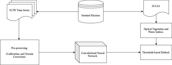
3. Proposed Method
- a novel deep learning architecture, called W-Net because of its W-shaped structure;
- the deep learning data fusion approach to the case of multi-temporal data;
- and a different segmentation map as reference, obtained by using the L2A product. In the previous work, we used a segmentation map, provided by the L2A product that included a huge number of invalid pixels.
4. Experimental Results
4.1. Classification Metrics
4.2. Compared Methods
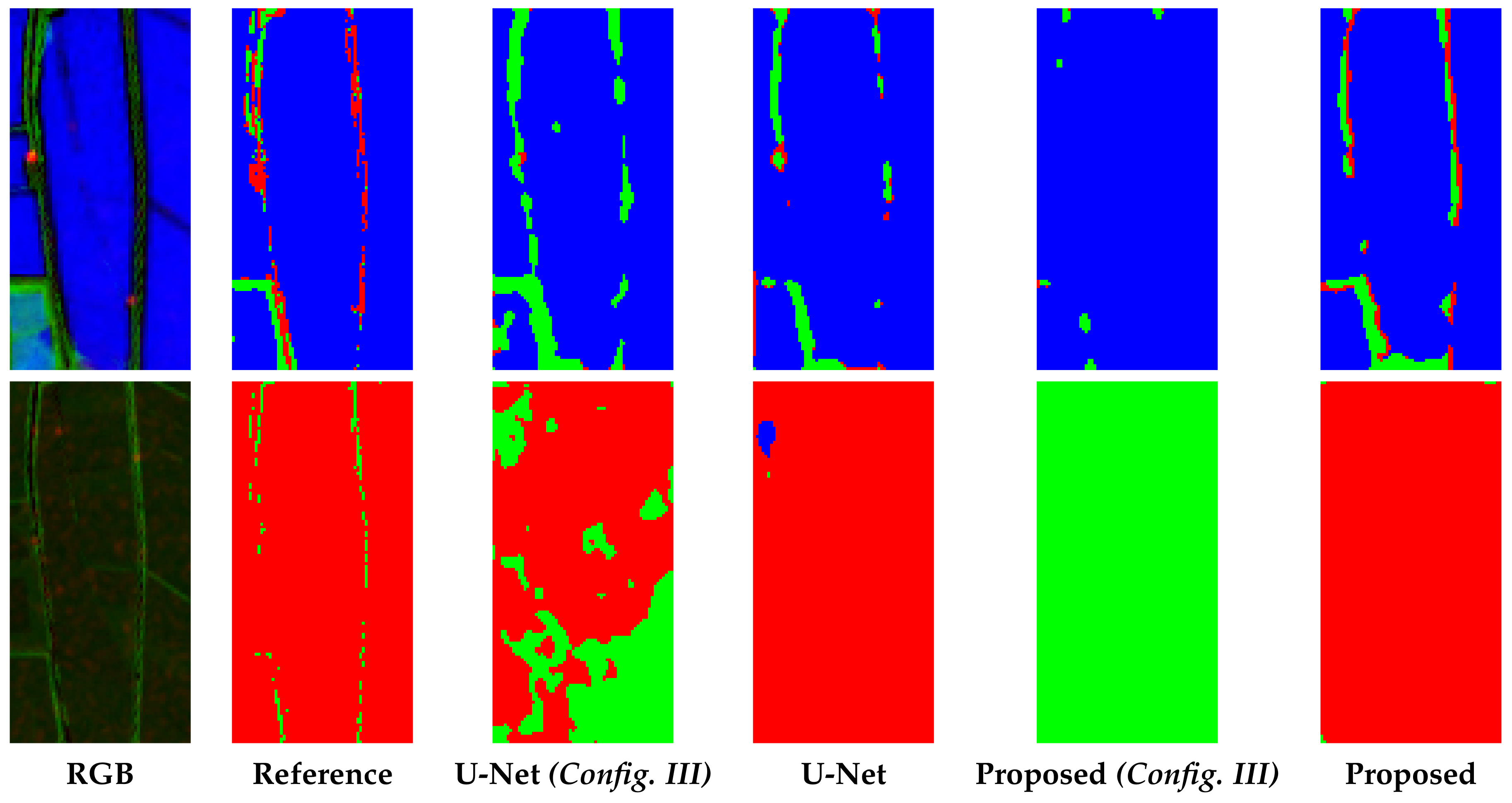
4.3. Numerical and Visual Results
5. Discussion
5.1. Single Date and Multi Date
5.2. Computation Time, Number of Parameters and Memory Occupation
6. Conclusions
Author Contributions
Funding
Acknowledgments
Conflicts of Interest
References
- Beck, L.R.; Lobitz, B.M.; Wood, B.L. Remote sensing and human health: new sensors and new opportunities. Emerg. Infect. Dis. 2000, 6, 217. [Google Scholar] [CrossRef] [PubMed]
- Gao, H.; Birkett, C.; Lettenmaier, D.P. Global monitoring of large reservoir storage from satellite remote sensing. Water Resour. Res. 2012, 48. [Google Scholar] [CrossRef]
- Salas, E.A.L.; Boykin, K.G.; Valdez, R. Multispectral and texture feature application in image-object analysis of summer vegetation in Eastern Tajikistan Pamirs. Remote. Sens. 2016, 8, 78. [Google Scholar] [CrossRef]
- Adams, J.B.; Sabol, D.E.; Kapos, V.; Almeida Filho, R.; Roberts, D.A.; Smith, M.O.; Gillespie, A.R. Classification of multispectral images based on fractions of endmembers: Application to land-cover change in the Brazilian Amazon. Remote. Sens. Environ. 1995, 52, 137–154. [Google Scholar] [CrossRef]
- Pal, M.K.; Rasmussen, T.M.; Abdolmaleki, M. Multiple Multi-Spectral Remote Sensing Data Fusion and Integration for Geological Mapping. In Proceedings of the 2019 10th Workshop on Hyperspectral Imaging and Signal Processing: Evolution in Remote Sensing (WHISPERS), Amsterdam, The Netherlands, 24–26 September 2019; pp. 1–5. [Google Scholar]
- Gargiulo, M.; Dell’Aglio, D.A.G.; Iodice, A.; Riccio, D.; Ruello, G. A CNN-Based Super-Resolution Technique for Active Fire Detection on Sentinel-2 Data. arXiv 2019, arXiv:1906.10413. [Google Scholar]
- Carlson, T.N.; Ripley, D.A. On the relation between NDVI, fractional vegetation cover, and leaf area index. Remote. Sens. Environ. 1997, 62, 241–252. [Google Scholar] [CrossRef]
- Maselli, F.; Chiesi, M.; Pieri, M. A new method to enhance the spatial features of multitemporal NDVI image series. IEEE Trans. Geosci. Remote. Sens. 2019, 57, 4967–4979. [Google Scholar] [CrossRef]
- Manzo, C.; Mei, A.; Fontinovo, G.; Allegrini, A.; Bassani, C. Integrated remote sensing for multi-temporal analysis of anthropic activities in the south-east of Mt. Vesuvius National Park. J. Afr. Earth Sci. 2016, 122, 63–78. [Google Scholar] [CrossRef]
- McFeeters, S.K. The use of the Normalized Difference Water Index (NDWI) in the delineation of open water features. Int. J. Remote. Sens. 1996, 17, 1425–1432. [Google Scholar] [CrossRef]
- Rokni, K.; Ahmad, A.; Solaimani, K.; Hazini, S. A new approach for detection of surface water changes based on principal component analysis of multitemporal normalized difference water index. J. Coast. Res. 2016, 32, 443–451. [Google Scholar]
- Gargiulo, M.; Mazza, A.; Gaetano, R.; Ruello, G.; Scarpa, G. A CNN-based fusion method for super-resolution of Sentinel-2 data. In Proceedings of the IGARSS 2018—2018 IEEE International Geoscience and Remote Sensing Symposium, Valencia, Spain, 22–27 July 2018; pp. 4713–4716. [Google Scholar]
- Nagler, T.; Rott, H.; Hetzenecker, M.; Wuite, J.; Potin, P. The Sentinel-1 Mission: New Opportunities for Ice Sheet Observations. Remote Sens. 2015, 7, 9371–9389. [Google Scholar] [CrossRef]
- Bazzi, H.; Baghdadi, N.; El Hajj, M.; Zribi, M.; Minh, D.H.T.; Ndikumana, E.; Courault, D.; Belhouchette, H. Mapping paddy rice using Sentinel-1 SAR time series in Camargue, France. Remote. Sens. 2019, 11, 887. [Google Scholar] [CrossRef]
- Amitrano, D.; Di Martino, G.; Iodice, A.; Riccio, D.; Ruello, G. Unsupervised rapid flood mapping using Sentinel-1 GRD SAR images. IEEE Trans. Geosci. Remote. Sens. 2018, 56, 3290–3299. [Google Scholar] [CrossRef]
- Abdikan, S.; Sanli, F.B.; Ustuner, M.; Calò, F. Land cover mapping using sentinel-1 SAR data. Int. Arch. Photogramm. Remote. Sens. Spat. Inf. Sci. 2016, 41, 757. [Google Scholar] [CrossRef]
- Liu, W.; Yang, J.; Li, P.; Han, Y.; Zhao, J.; Shi, H. A novel object-based supervised classification method with active learning and random forest for PolSAR imagery. Remote. Sens. 2018, 10, 1092. [Google Scholar] [CrossRef]
- Santana-Cedrés, D.; Gomez, L.; Trujillo, A.; Alemán-Flores, M.; Deriche, R.; Alvarez, L. Supervised Classification of Fully PolSAR Images Using Active Contour Models. IEEE Geosci. Remote. Sens. Lett. 2019, 16, 1165–1169. [Google Scholar] [CrossRef]
- Lu, L.; Zhang, J.; Huang, G.; Su, X. Land cover classification and height extraction experiments using Chinese airborne X-band PolInSAR system in China. Int. J. Image Data Fusion 2016, 7, 282–294. [Google Scholar] [CrossRef]
- Biondi, F. Multi-chromatic analysis polarimetric interferometric synthetic aperture radar (MCA-PolInSAR) for urban classification. Int. J. Remote. Sens. 2019, 40, 3721–3750. [Google Scholar] [CrossRef]
- Brakenridge, R.; Anderson, E. MODIS-based flood detection, mapping and measurement: the potential for operational hydrological applications. In Transboundary Floods: Reducing Risks through Flood Management; Springer: Dordrecht, The Netherlands, 2006; pp. 1–12. [Google Scholar]
- Yoon, D.H.; Nam, W.H.; Lee, H.J.; Hong, E.M.; Kim, T.; Kim, D.E.; Shin, A.K.; Svoboda, M.D. Application of evaporative stress index (ESI) for satellite-based agricultural drought monitoring in South Korea. J. Korean Soc. Agric. Eng. 2018, 60, 121–131. [Google Scholar]
- Kim, J.C.; Jung, H.S. Application of landsat tm/etm+ images to snow variations detection by volcanic activities at southern volcanic zone, Chile. Korean J. Remote. Sens. 2017, 33, 287–299. [Google Scholar]
- Murakami, T.; Ogawa, S.; Ishitsuka, N.; Kumagai, K.; Saito, G. Crop discrimination with multitemporal SPOT/HRV data in the Saga Plains, Japan. Int. J. Remote. Sens. 2001, 22, 1335–1348. [Google Scholar] [CrossRef]
- Gargiulo, M. Advances on CNN-based super-resolution of Sentinel-2 images. In Proceedings of the IGARSS 2019–2019 IEEE International Geoscience and Remote Sensing Symposium, Yokohama, Japan, 28 July–2 August 2019; pp. 3165–3168. [Google Scholar]
- Scarpa, G.; Gargiulo, M.; Mazza, A.; Gaetano, R. A CNN-based fusion method for feature extraction from sentinel data. Remote. Sens. 2018, 10, 236. [Google Scholar] [CrossRef]
- Whyte, A.; Ferentinos, K.P.; Petropoulos, G.P. A new synergistic approach for monitoring wetlands using Sentinels-1 and 2 data with object-based machine learning algorithms. Environ. Model. Softw. 2018, 104, 40–54. [Google Scholar] [CrossRef]
- Clerici, N.; Valbuena Calderón, C.A.; Posada, J.M. Fusion of Sentinel-1A and Sentinel-2A data for land cover mapping: a case study in the lower Magdalena region, Colombia. J. Maps 2017, 13, 718–726. [Google Scholar] [CrossRef]
- Kussul, N.; Lavreniuk, M.; Skakun, S.; Shelestov, A. Deep learning classification of land cover and crop types using remote sensing data. IEEE Geosci. Remote. Sens. Lett. 2017, 14, 778–782. [Google Scholar] [CrossRef]
- Stoian, A.; Poulain, V.; Inglada, J.; Poughon, V.; Derksen, D. Land Cover Maps Production with High Resolution Satellite Image Time Series and Convolutional Neural Networks: Adaptations and Limits for Operational Systems. Remote. Sens. 2019, 11, 1986. [Google Scholar] [CrossRef]
- Lang, F.; Yang, J.; Yan, S.; Qin, F. Superpixel segmentation of polarimetric synthetic aperture radar (sar) images based on generalized mean shift. Remote. Sens. 2018, 10, 1592. [Google Scholar] [CrossRef]
- Stutz, D.; Hermans, A.; Leibe, B. Superpixels: An evaluation of the state-of-the-art. Comput. Vis. Image Underst. 2018, 166, 1–27. [Google Scholar] [CrossRef]
- Ciecholewski, M. River channel segmentation in polarimetric SAR images: Watershed transform combined with average contrast maximisation. Expert Syst. Appl. 2017, 82, 196–215. [Google Scholar] [CrossRef]
- Cousty, J.; Bertrand, G.; Najman, L.; Couprie, M. Watershed cuts: Thinnings, shortest path forests, and topological watersheds. IEEE Trans. Pattern Anal. Mach. Intell. 2009, 32, 925–939. [Google Scholar] [CrossRef]
- Braga, A.M.; Marques, R.C.; Rodrigues, F.A.; Medeiros, F.N. A median regularized level set for hierarchical segmentation of SAR images. IEEE Geosci. Remote. Sens. Lett. 2017, 14, 1171–1175. [Google Scholar] [CrossRef]
- Jin, R.; Yin, J.; Zhou, W.; Yang, J. Level set segmentation algorithm for high-resolution polarimetric SAR images based on a heterogeneous clutter model. IEEE J. Sel. Top. Appl. Earth Obs. Remote. Sens. 2017, 10, 4565–4579. [Google Scholar] [CrossRef]
- Zhou, Y.; Wang, H.; Xu, F.; Jin, Y.Q. Polarimetric SAR image classification using deep convolutional neural networks. IEEE Geosci. Remote. Sens. Lett. 2016, 13, 1935–1939. [Google Scholar] [CrossRef]
- Gargiulo, M.; Dell’Aglio, D.A.; Iodice, A.; Riccio, D.; Ruello, G. Semantic Segmentation using Deep Learning: A case of study in Albufera Park, Valencia. In Proceedings of the 2019 IEEE International Workshop on Metrology for Agriculture and Forestry (MetroAgriFor), Naples, Italy, 24–26 October 2019; pp. 134–138. [Google Scholar]
- D’Odorico, P.; Gonsamo, A.; Damm, A.; Schaepman, M.E. Experimental evaluation of Sentinel-2 spectral response functions for NDVI time-series continuity. IEEE Trans. Geosci. Remote. Sens. 2013, 51, 1336–1348. [Google Scholar] [CrossRef]
- Gargiulo, M.; Mazza, A.; Gaetano, R.; Ruello, G.; Scarpa, G. Fast Super-Resolution of 20 m Sentinel-2 Bands Using Convolutional Neural Networks. Remote. Sens. 2019, 11, 2635. [Google Scholar] [CrossRef]
- Gao, L.; Song, W.; Dai, J.; Chen, Y. Road extraction from high-resolution remote sensing imagery using refined deep residual convolutional neural network. Remote. Sens. 2019, 11, 552. [Google Scholar] [CrossRef]
- Shao, Z.; Pan, Y.; Diao, C.; Cai, J. Cloud detection in remote sensing images based on multiscale features-convolutional neural network. IEEE Trans. Geosci. Remote. Sens. 2019, 57, 4062–4076. [Google Scholar] [CrossRef]
- Ronneberger, O.; Fischer, P.; Brox, T. U-net: Convolutional networks for biomedical image segmentation. In Proceedings of the International Conference on Medical Image Computing and Computer-Assisted Intervention, Munich, Germany, 5–9 October 2015; Springer: Munich, Germany, 2015; pp. 234–241. [Google Scholar]
- Xia, X.; Kulis, B. W-net: A deep model for fully unsupervised image segmentation. arXiv 2017, arXiv:1711.08506. [Google Scholar]
- Larsson, G.; Maire, M.; Shakhnarovich, G. Fractalnet: Ultra-deep neural networks without residuals. arXiv 2016, arXiv:1605.07648. [Google Scholar]
- Zhao, X.; Yuan, Y.; Song, M.; Ding, Y.; Lin, F.; Liang, D.; Zhang, D. Use of Unmanned Aerial Vehicle Imagery and Deep Learning UNet to Extract Rice Lodging. Sensors 2019, 19, 3859. [Google Scholar] [CrossRef]
- Rahman, M.A.; Wang, Y. Optimizing intersection-over-union in deep neural networks for image segmentation. In Proceedings of the International Symposium on Visual Computing, Las Vegas, NV, USA, 12–14 December 2016; Springer: Las Vegas, NV, USA, 2016; pp. 234–244. [Google Scholar]
- Kingma, D.P.; Ba, J. Adam: A method for stochastic optimization. arXiv 2014, arXiv:1412.6980. [Google Scholar]
- Glorot, X.; Bengio, Y. Understanding the difficulty of training deep feedforward neural networks. In Proceedings of the Thirteenth International Conference on Artificial Intelligence and Statistics, Sardinia, Italy, 13–15 May 2010; pp. 249–256. [Google Scholar]
- Dong, C.; Loy, C.C.; He, K.; Tang, X. Image super-resolution using deep convolutional networks. IEEE Trans. Pattern Anal. Mach. Intell. 2015, 38, 295–307. [Google Scholar] [CrossRef] [PubMed]
- Badrinarayanan, V.; Kendall, A.; Cipolla, R. Segnet: A deep convolutional encoder-decoder architecture for image segmentation. IEEE Trans. Pattern Anal. Mach. Intell. 2017, 39, 2481–2495. [Google Scholar] [CrossRef] [PubMed]
- Chaurasia, A.; Culurciello, E. Linknet: Exploiting encoder representations for efficient semantic segmentation. In Proceedings of the 2017 IEEE Visual Communications and Image Processing (VCIP), St. Petersburg, FL, USA, 10–13 December 2017; pp. 1–4. [Google Scholar]
- Kirillov, A.; Girshick, R.; He, K.; Dollár, P. Panoptic feature pyramid networks. In Proceedings of the IEEE Conference on Computer Vision and Pattern Recognition, Long Beach, CA, USA, 16–20 June 2019; pp. 6399–6408. [Google Scholar]
- Ienco, D.; Gaetano, R.; Dupaquier, C.; Maurel, P. Land cover classification via multitemporal spatial data by deep recurrent neural networks. IEEE Geosci. Remote. Sens. Lett. 2017, 14, 1685–1689. [Google Scholar] [CrossRef]


| Data | Type | Satellite | Spatial Resolution | # Images | Minimum Revisit Time | Considered Revisit Time | Polarization Bands |
|---|---|---|---|---|---|---|---|
| Satellite Images | Synthetic Aperture Radar (SAR) | S-1 | 10 m | 36 | 6 days | 6 days * | VV + VH |
| Multi-Spectral | S-2 | 10 m | 12 | 5 days | 1 month | , , |
| Specifications | Sentinel-1A Data |
|---|---|
| Acquisition orbit | Descending |
| Imaging mode | IW |
| Imaging frequency | C-band ( GHz) |
| Polarization | VV, VH |
| Data Product | Level-1 GRDH |
| Resolution Mode | 10-m |
| Spatial Resolution [m] | Spectral Bands (Bands Number) | Wavelength Range [m] |
|---|---|---|
| 10 | Blue (2), Green (3), Red (4), and NIR (8) | 0.490–0.842 |
| 20 | Vegetation Red Edge (5,6,7, 8A) and SWIR (11,12) | 0.705–2.190 |
| 60 | Coastal Aerosol (1), Water Vapour (9), and SWIR (10) | 0.443–1.375 |
| Configurations | No. Input Bands | Description | Considered Times |
|---|---|---|---|
| I | 1 | 1 | |
| II | 1 | 1 | |
| III | 2 | 1 | |
| IV | 6 | 0, 1, 2 |
| Models | # Parameters | Time per Epoch [s] | Memory |
|---|---|---|---|
| ShallowNet | 45.6 k | 32.0 | 191 k |
| SegNet | 1.8 M | 63.2 | 7.17 M |
| FPN | 6.9 M | 711.0 | 26.8 M |
| LinkNet | 4.1 M | 428.8 | 30.9 M |
| U-Net | 8 M | 209.2 | 30.9 M |
| Proposed | 1.2 M | 89.6 | 4.75 M |
| Methods | Metrics | |||
|---|---|---|---|---|
| Accuracy | Precision | Recall | F1 | |
| ShallowNet | 0.8271 | 0.7743 | 0.7651 | 0.7639 |
| SegNet | 0.8240 | 0.7691 | 0.7610 | 0.7596 |
| FPN | 0.8418 | 0.8107 | 0.7746 | 0.7801 |
| LinkNet | 0.8310 | 0.8083 | 0.7623 | 0.7667 |
| U-Net | 0.8846 | 0.8567 | 0.8318 | 0.8405 |
| Proposed | 0.9121 | 0.8860 | 0.8682 | 0.8762 |
| Methods | Configuration | Metrics | Time per Epoch | |||
|---|---|---|---|---|---|---|
| Accuracy | Precision | Recall | F1 | |||
| U-Net | III | 0.7938 | 0.7503 | 0.7002 | 0.6812 | 177.6 |
| U-Net | IV | 0.8846 | 0.8567 | 0.8318 | 0.8405 | 209.2 |
| Proposed | I | 0.7162 | 0.7306 | 0.6091 | 0.5832 | 70.2 |
| Proposed | II | 0.7263 | 0.6865 | 0.6280 | 0.5806 | 63.6 |
| Proposed | III | 0.735 | 0.6563 | 0.6299 | 0.6213 | 81.0 |
| Proposed | IV | 0.9121 | 0.8860 | 0.8682 | 0.8762 | 89.6 |
© 2020 by the authors. Licensee MDPI, Basel, Switzerland. This article is an open access article distributed under the terms and conditions of the Creative Commons Attribution (CC BY) license (http://creativecommons.org/licenses/by/4.0/).
Share and Cite
Gargiulo, M.; Dell’Aglio, D.A.G.; Iodice, A.; Riccio, D.; Ruello, G. Integration of Sentinel-1 and Sentinel-2 Data for Land Cover Mapping Using W-Net. Sensors 2020, 20, 2969. https://doi.org/10.3390/s20102969
Gargiulo M, Dell’Aglio DAG, Iodice A, Riccio D, Ruello G. Integration of Sentinel-1 and Sentinel-2 Data for Land Cover Mapping Using W-Net. Sensors. 2020; 20(10):2969. https://doi.org/10.3390/s20102969
Chicago/Turabian StyleGargiulo, Massimiliano, Domenico A. G. Dell’Aglio, Antonio Iodice, Daniele Riccio, and Giuseppe Ruello. 2020. "Integration of Sentinel-1 and Sentinel-2 Data for Land Cover Mapping Using W-Net" Sensors 20, no. 10: 2969. https://doi.org/10.3390/s20102969
APA StyleGargiulo, M., Dell’Aglio, D. A. G., Iodice, A., Riccio, D., & Ruello, G. (2020). Integration of Sentinel-1 and Sentinel-2 Data for Land Cover Mapping Using W-Net. Sensors, 20(10), 2969. https://doi.org/10.3390/s20102969