Monitoring of the Static and Dynamic Displacements of Railway Bridges with the Use of Inertial Sensors


Abstract
1. Introduction
- validate design conceptions,
- evaluate condition state,
- assess behavior under high-speed train loadings,
- carry out damage detection based on vibration analysis.
2. Description of Monitoring System
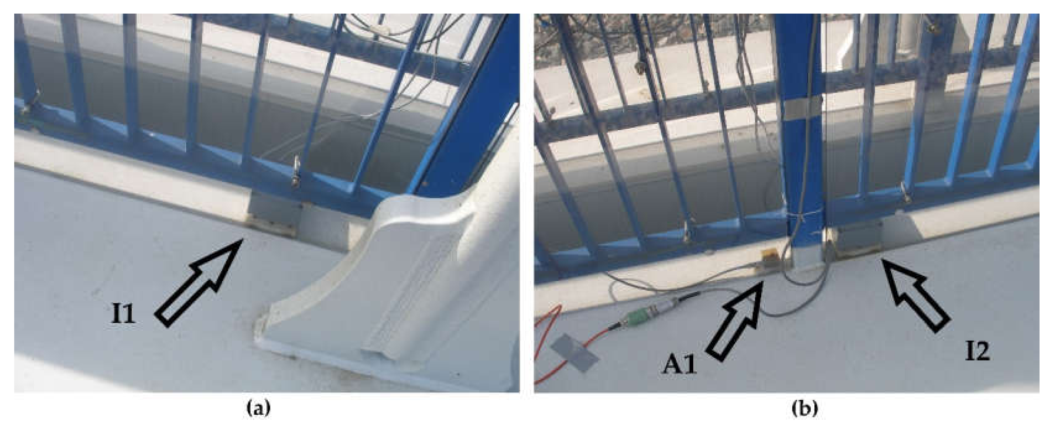
2.1. Hardware
- uniaxial gravity inclinometer with measuring range of ±1°;
- triaxial piezoelectric accelerometer with measuring range of ±5g;
- MEMS-type triaxial accelerometer with measuring range of ±3g;
- resistance strain gauge;
- temperature sensor with a measuring range from −55 °C to +125 °C.
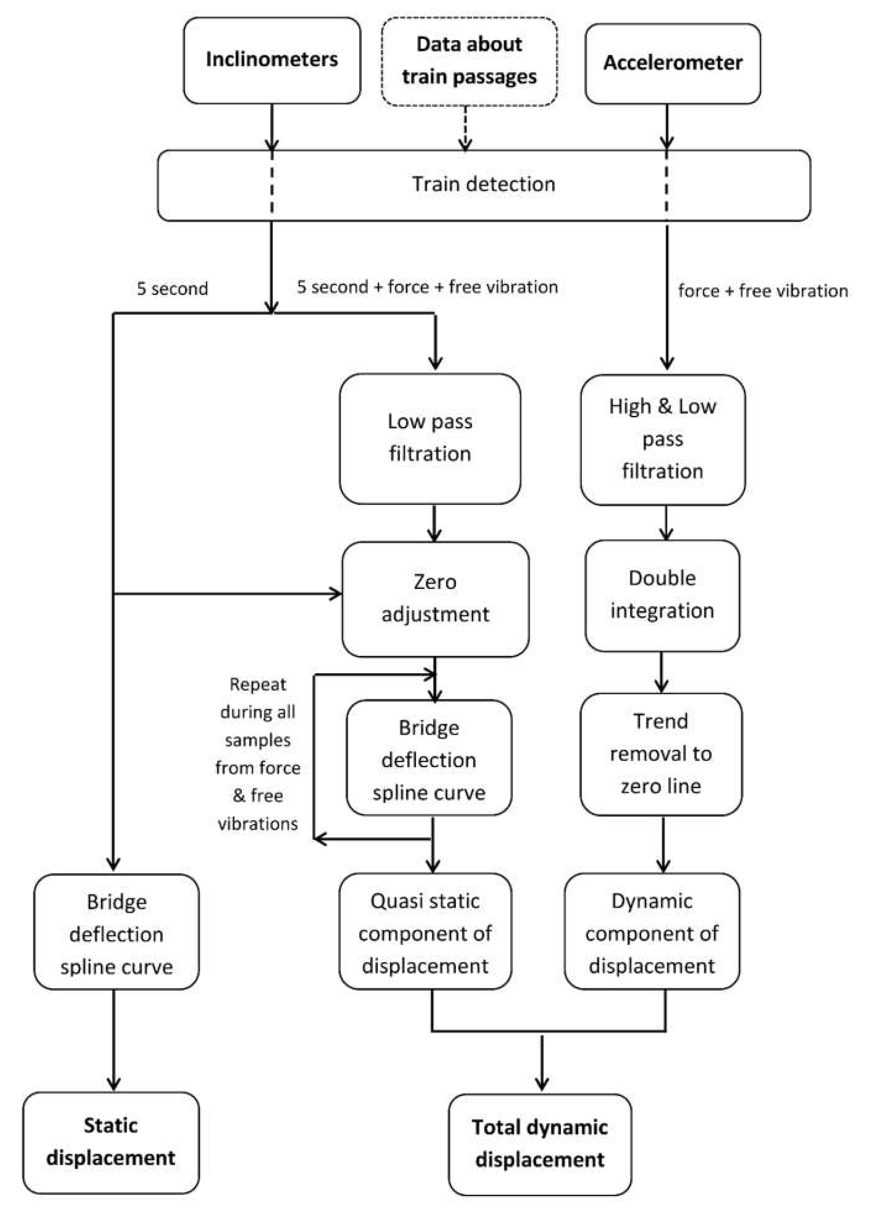
2.2. Algorithm and Software
- (1)
- 5 s time registration of all signals before the train enters the bridge;
- (2)
- force vibration registration when the train is on the bridge;
- (3)
- free vibration registration after train leaves the bridge.
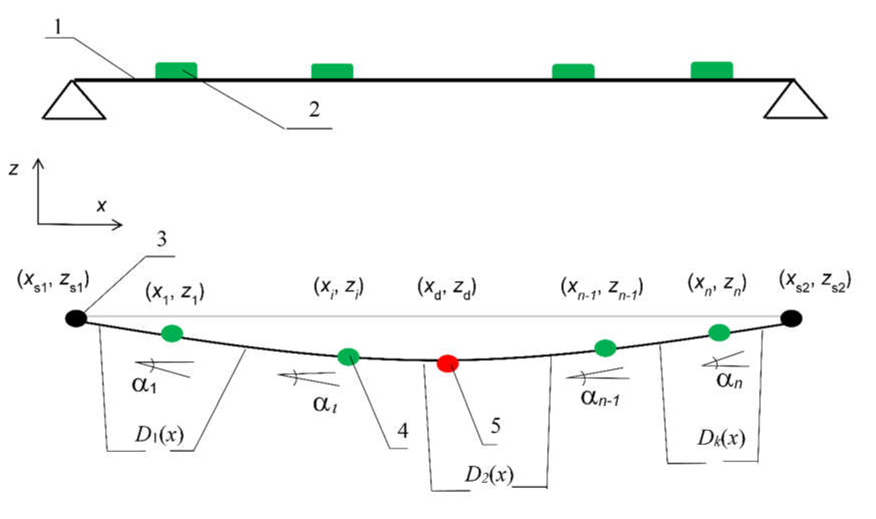
2.2.1. Static Displacement Determination
- points of inclinometers’ location (coordinates (xi,zi)) with Dj(x) curve:
- 2.
- points of connection of curves Dj(x) and Dj+1(x):
- 3.
- support points (coordinates (xs1, zs1) or (xs2, zs2)) belonging to curve D1(x) or Dk(x):
- tangent to the angle indicated by the inclinometer, according to Equation (2);
- smooth curves (first derivative), according to Equation (3);
- curves with continuous curvature (second derivation), according to Equation (4);
- curve continuity, according to Equation (5);
- a known (zero) coordinate of support zs, according to Equation (6);
- angle on the outer support equal to the indications of the nearest inclinometer, according to Equation (7).
2.2.2. Dynamic Displacement Determination
3. The First Tests
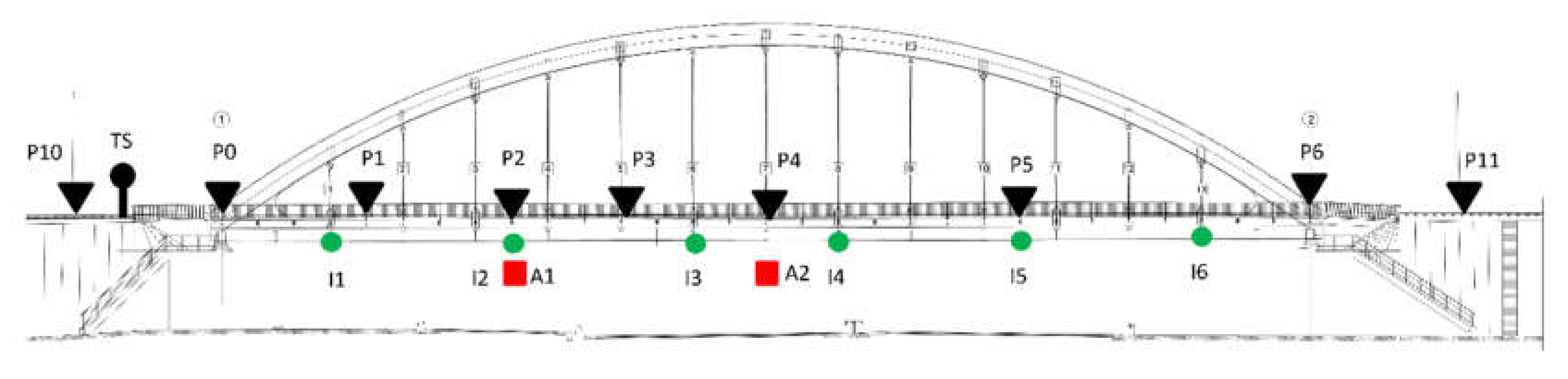
3.1. The Tested Bridge
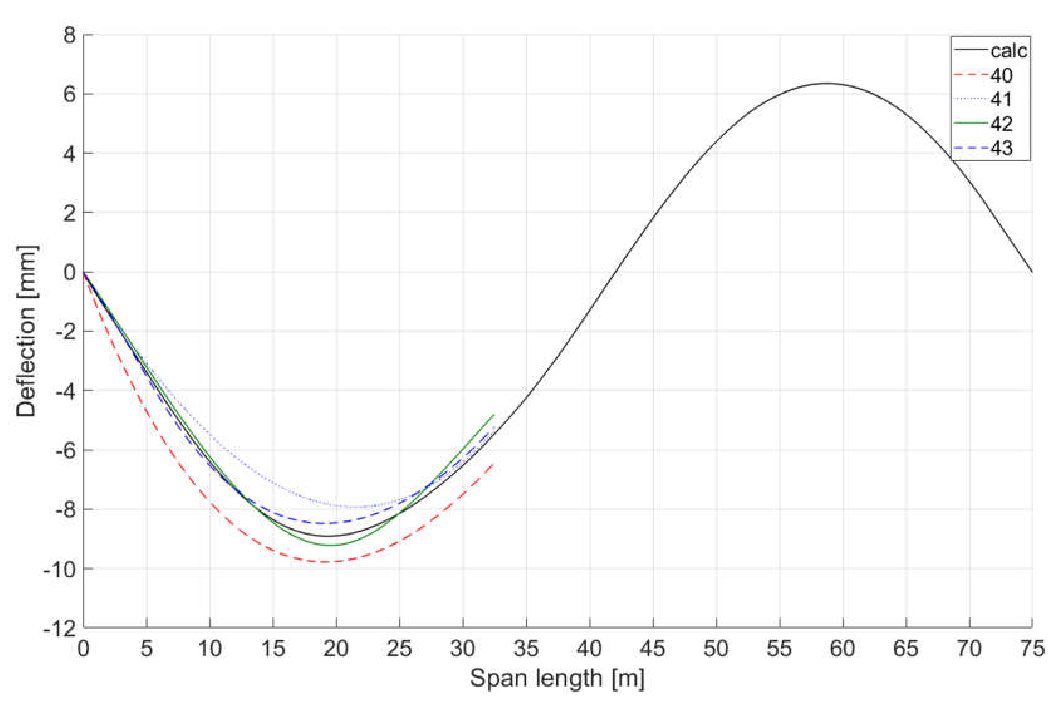
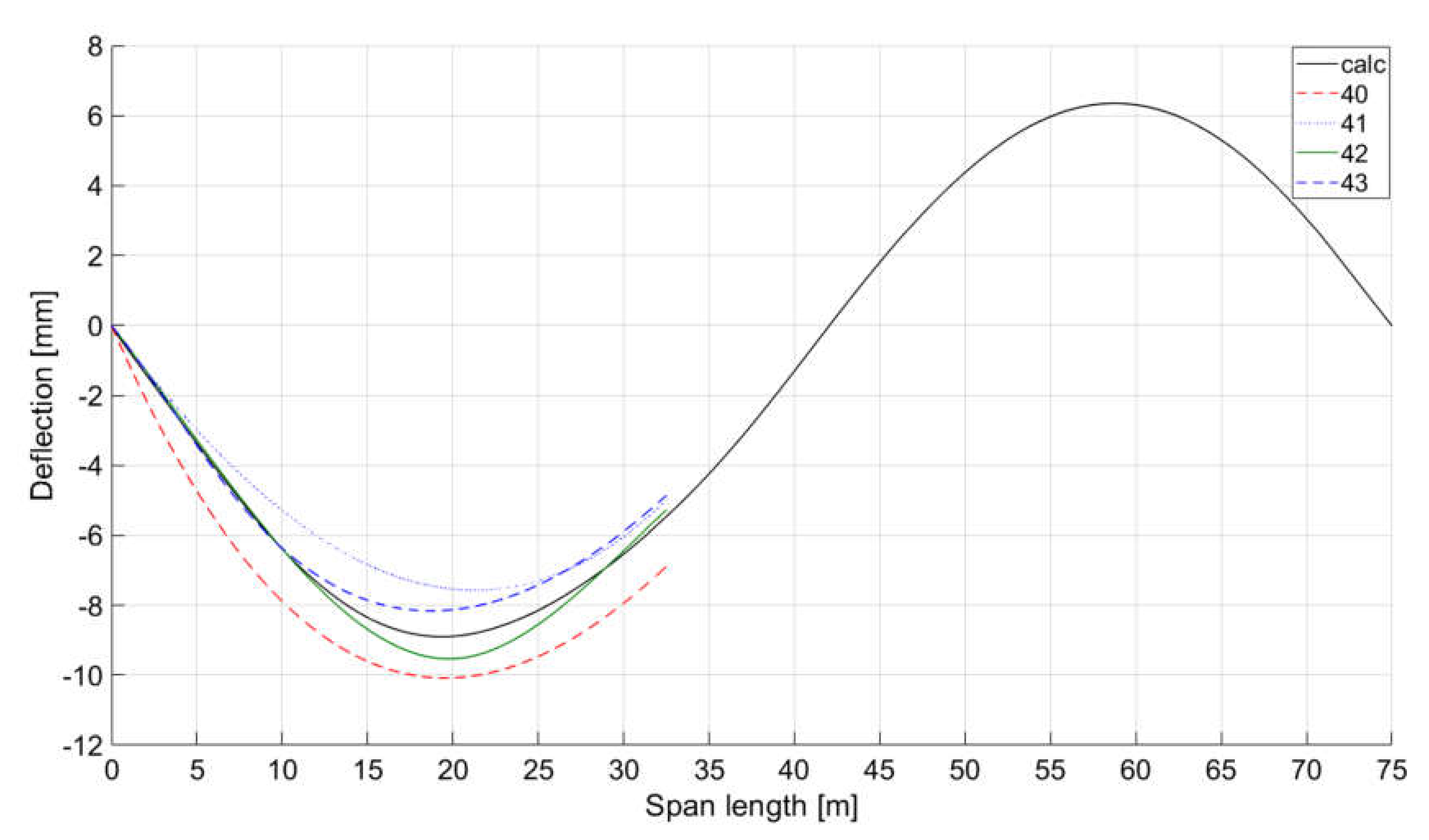
3.2. Algorithm Adaptation to the Tested Bridge
- a single 3° curve (designation 40),
- a single 3° curve with an angle of rotation at the support equal to that of inclinometer I1 (designation 41),
- two spline curves connected together at the point of location of inclinometer I2 with an angle of rotation at a support equal to that of inclinometer I1 (designation 42),
- three spline curves combined at the points of the locations of inclinometers I1 and I2 with an angle of rotation at a support equal to that of inclinometer I1 (designation 43).
4. Results of the Bridge Monitoring
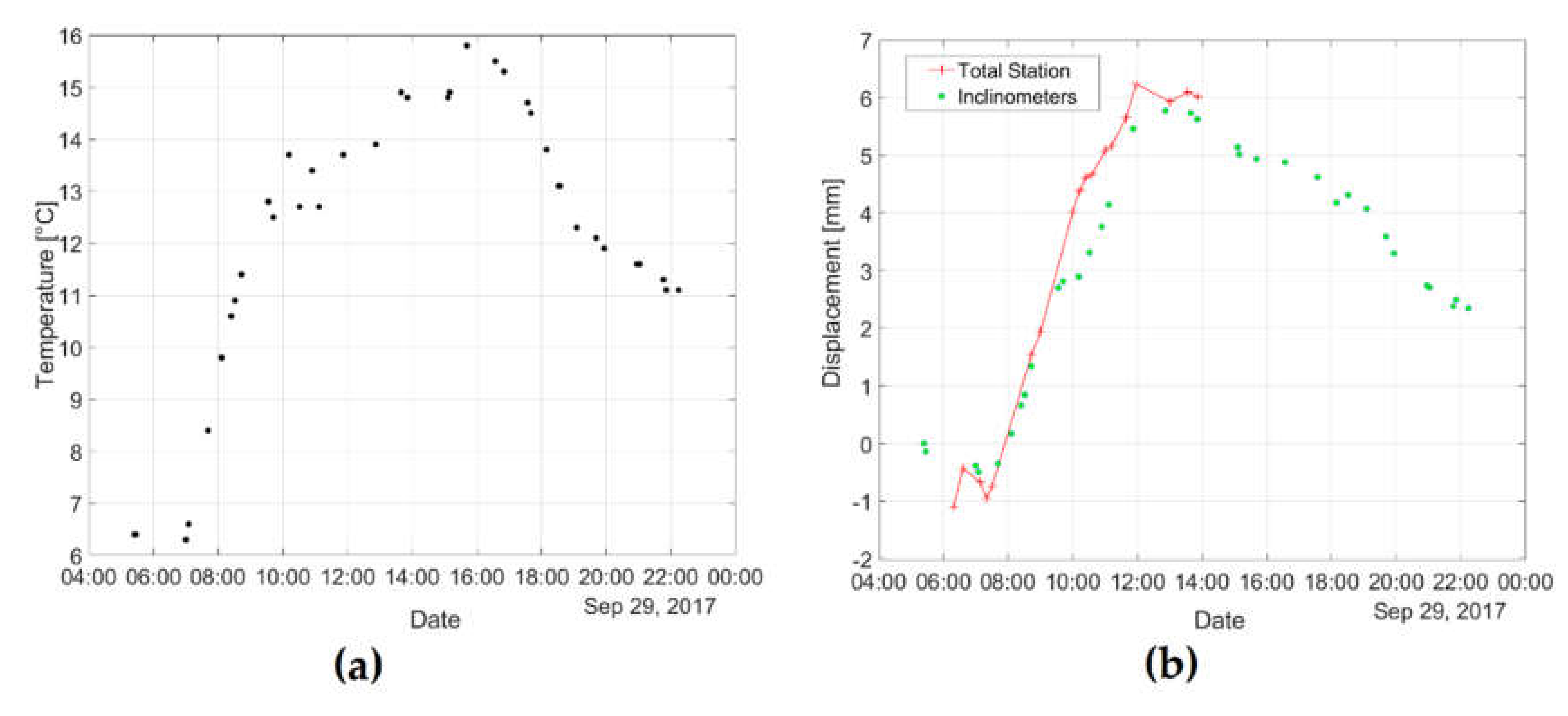
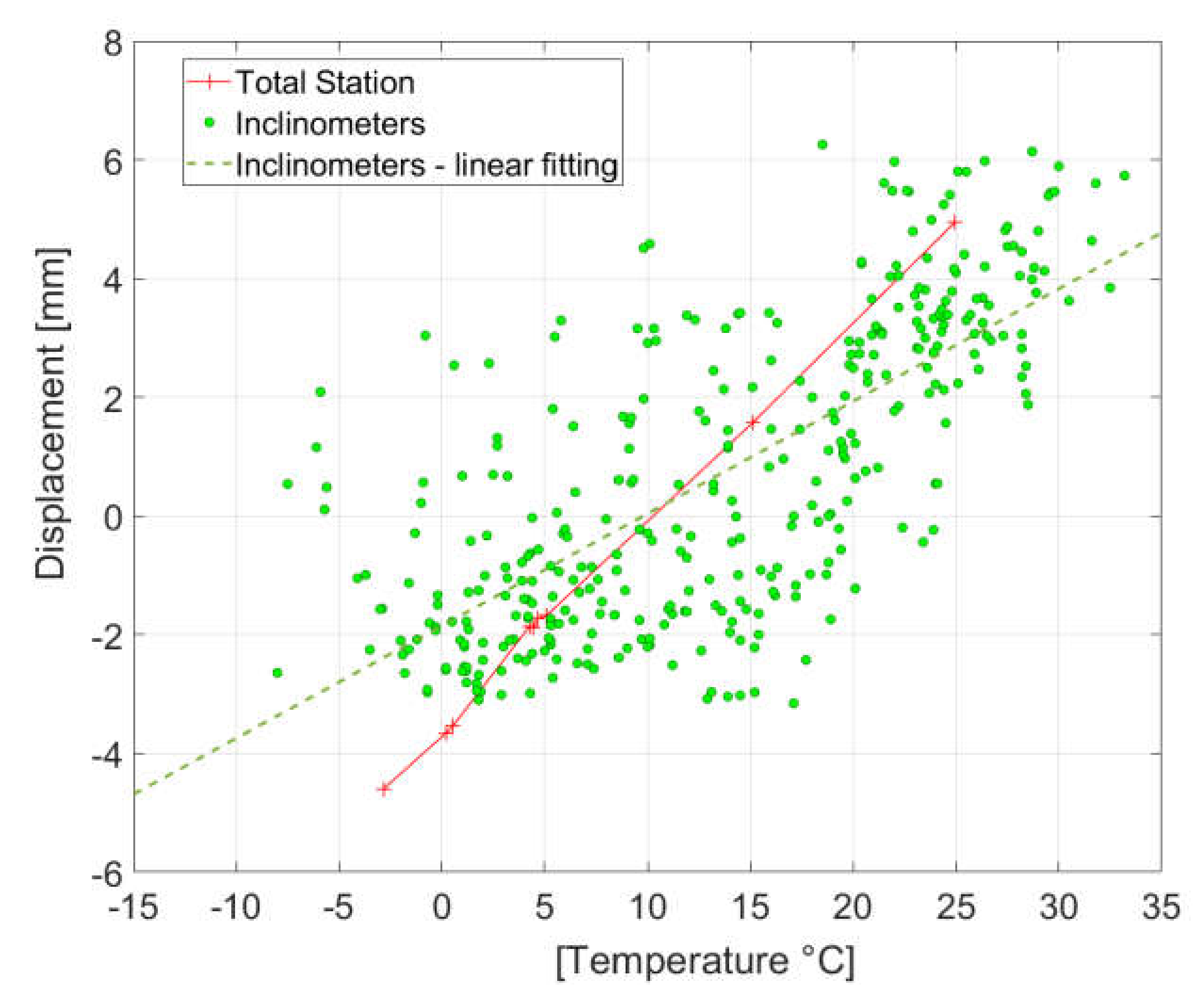
4.1. Static Displacement Measurement Results
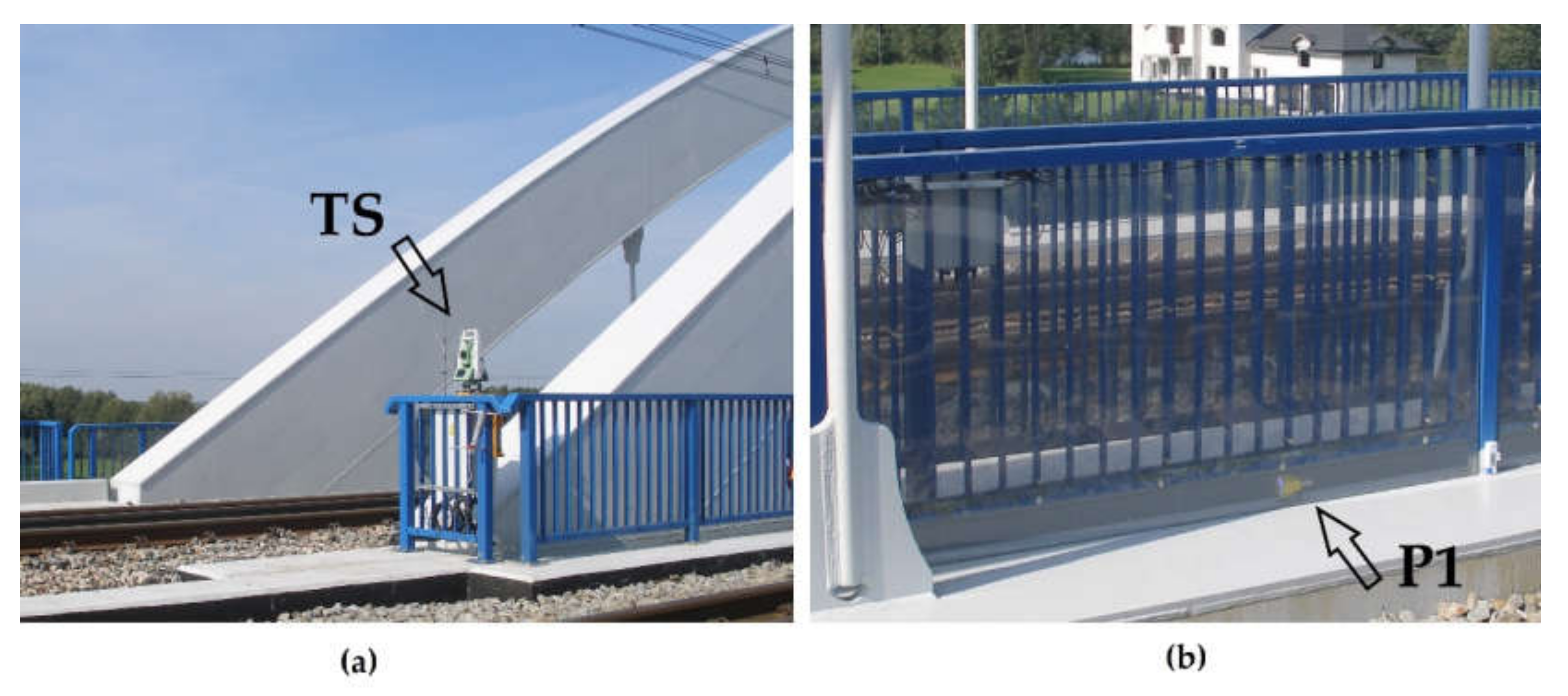
- tachymetric measurement before arrival of the train,
- 5 s inclinometer readings before the train reaches the bridge,
- calculation of displacement for both methods and comparison of results.
- uniform change in the temperature of the bridge (steel structure and concrete plate) generates mainly longitudinal deformation;
- temperature change of steel structure (excluding concrete plate) causes bending mode with 6.4 mm for 10 °C at the middle of the span length;
- temperature change of lateral wall of steel girder creates torsional deformation of the bridge.
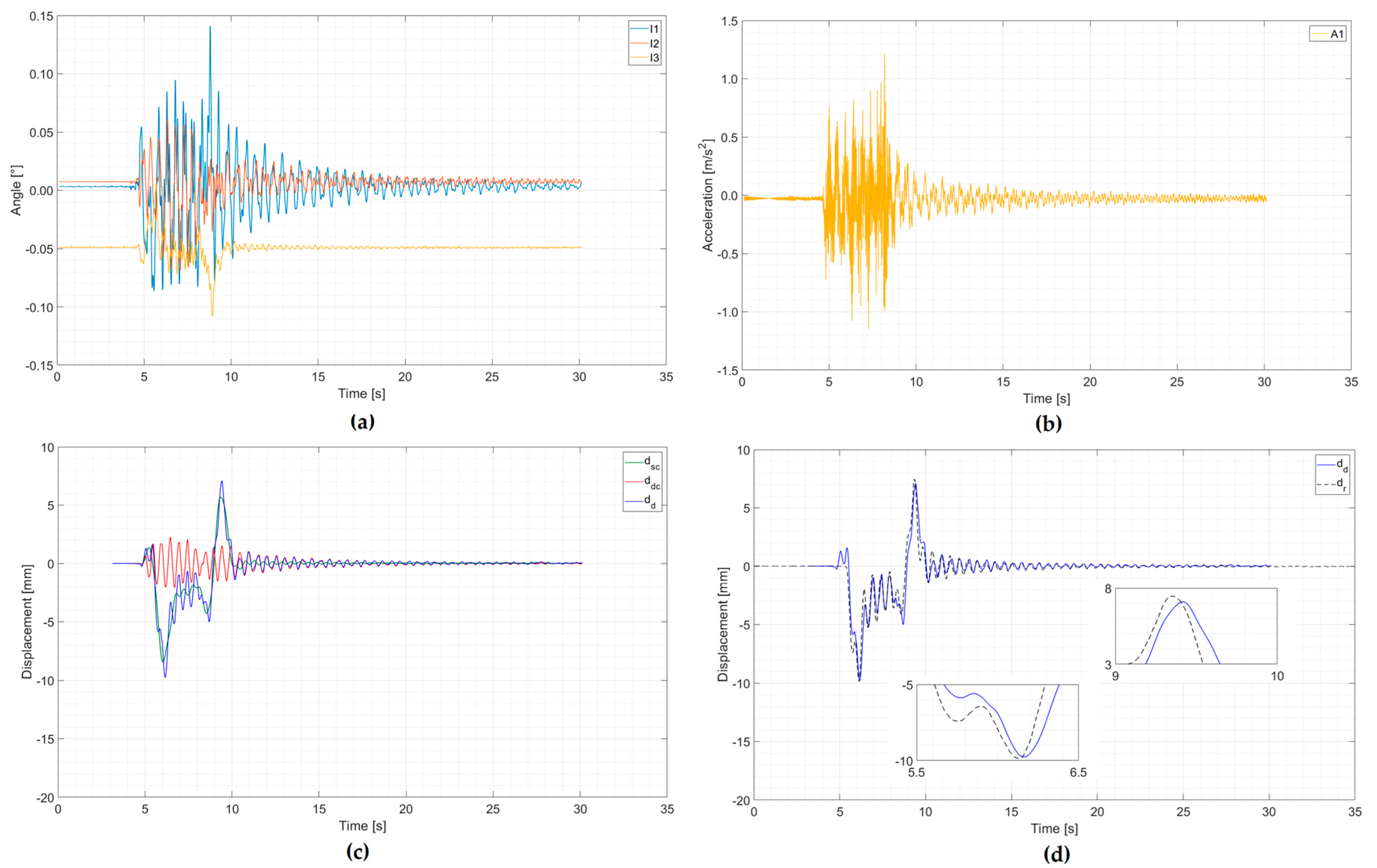
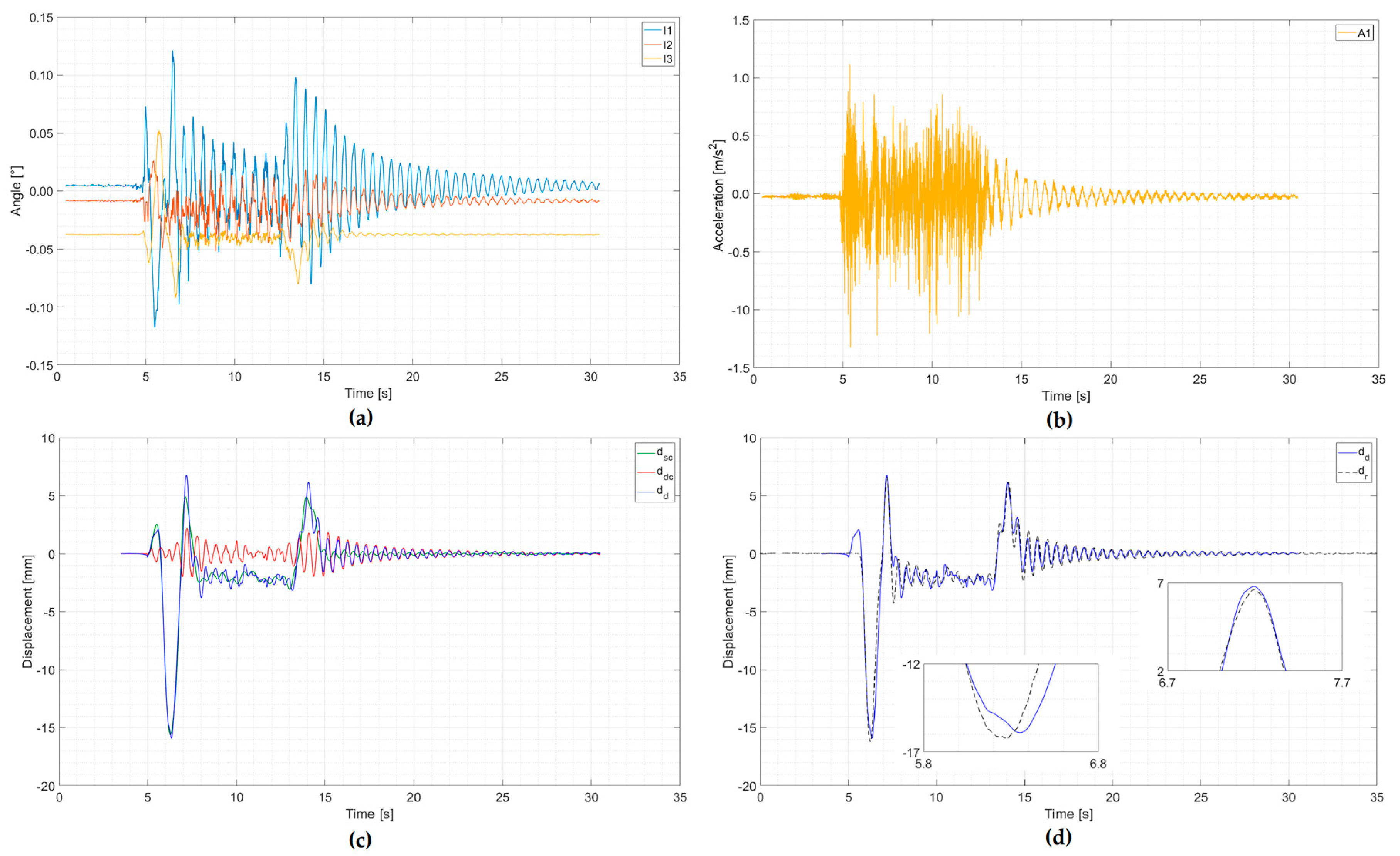
4.2. Dynamic Displacement Measurement Results—Single Train Passages
- Multiple-unit train: ∆min = 0.13 mm, ∆min/dr min= 1.3%, ∆max = 0.36 mm, ∆max/dr max= 4.8%;
- Separate locomotive and cars: ∆min = 0.36 mm, ∆min/dr min= 2.2%, ∆max = 0.22 mm, ∆max/dr max= 3.3%.
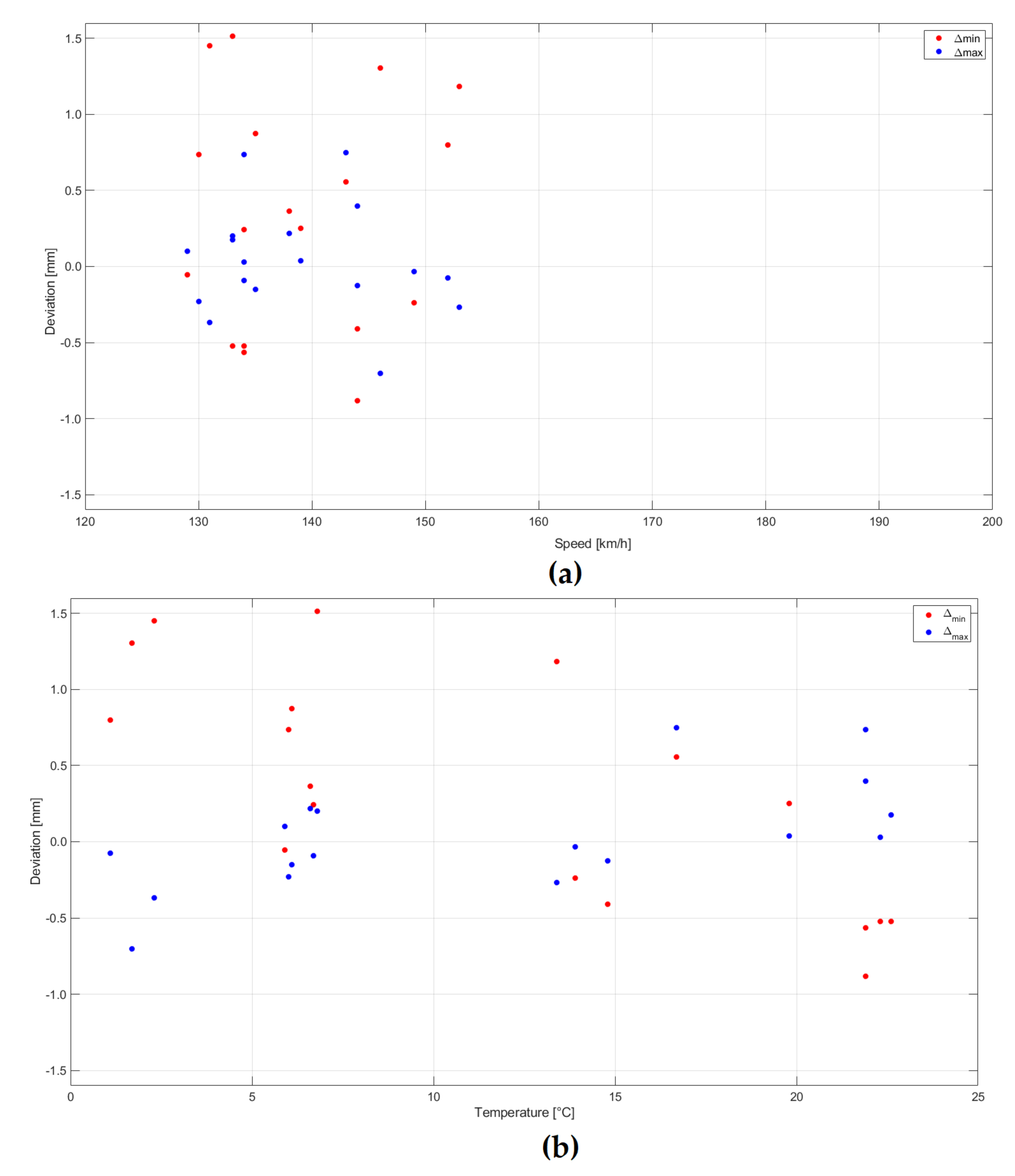
4.3. Dynamic Displacement Measurement Results—Continuous Monitoring
5. Conclusions
Author Contributions
Funding
Acknowledgments
Conflicts of Interest
References
- Frýba, L. A rough assessment of railway bridges for high speed trains. Eng. Struct. 2001, 23, 548–556. [Google Scholar] [CrossRef]
- Frýba, L. Dynamics of Railway Bridges; Thomas Telford Limited: London, UK, 1996; ISBN 978-0-7277-3471-6. [Google Scholar]
- Yang, Y.B.; Yau, J.D.; Wu, Y.S. Vehicle-Bridge Interaction Dynamics. With Applications to High-Speed Railways; World Scientific: Singapore, 2004. [Google Scholar]
- Ehrhart, M.; Lienhart, W. Monitoring of Civil Engineering Structures using a State-of-the-art Image Assisted Total Station: Journal of Applied Geodesy. Available online: https://www.degruyter.com/view/j/jag.2015.9.issue-3/jag-2015-0005/jag-2015-0005.xml (accessed on 11 June 2019).
- Parker, D.H. Nondestructive Testing and Monitoring of Stiff Large-Scale Structures by Measuring 3D Coordinates of Cardinal Points Using Electronic Distance Measurements in a Trilateration Architecture; International Society for Optics and Photonics: Portland, OR, USA, 2017. [Google Scholar]
- Psimoulis, P.A.; Stiros, S.C. Measurement of deflections and of oscillation frequencies of engineering structures using Robotic Theodolites (RTS). Eng. Struct. 2007, 29, 3312–3324. [Google Scholar] [CrossRef]
- Yigit, C.O.; Gurlek, E. Experimental testing of high-rate GNSS precise point positioning (PPP) method for detecting dynamic vertical displacement response of engineering structures. Geomat. Nat. Hazards Risk 2017, 8, 893–904. [Google Scholar] [CrossRef]
- Lazecky, M.; Perissin, D.; Bakon, M.; de Sousa, J.M.; Hlavacova, I.; Real, N. Potential of satellite InSAR techniques for monitoring of bridge deformations. 2015 Jt. Urban Remote Sens. Event JURSE 2015. [Google Scholar] [CrossRef]
- Zhao, J.; Wu, J.; Ding, X.; Wang, M. Elevation Extraction and Deformation Monitoring by Multitemporal InSAR of Lupu Bridge in Shanghai. Remote Sens. 2017, 9, 897. [Google Scholar] [CrossRef]
- Feng, D.; Feng, M.Q. Vision-based multipoint displacement measurement for structural health monitoring. Struct. Control Health Monit. 2016, 23, 876–890. [Google Scholar] [CrossRef]
- Sabato, A.; Niezrecki, C. Feasibility of digital image correlation for railroad tie inspection and ballast support assessment. Measurement 2017, 103, 93–105. [Google Scholar] [CrossRef]
- Waterfall, P.W.; MacDonald, J.H.G.; McCormick, N.J. Targetless precision monitoring of road and rail bridges using video cameras. In Proceedings of the Sixth International Conference on Bridge Maintenance, Safety and Management (IABMAS 2012), Stresa Lake Maggiore, Italy, 8–12 July 2012; pp. 3976–3982. [Google Scholar]
- Matsuoka, K.; Collina, A.; Somaschini, C.; Sogabe, M. Influence of local deck vibrations on the evaluation of the maximum acceleration of a steel-concrete composite bridge for a high-speed railway. Eng. Struct. 2019, 200, 109736. [Google Scholar] [CrossRef]
- Bačinskas, D.; Kamaitis, Z.; Kilikevičius, A. A sensor instrumentation method for dynamic monitoring of railway bridges. J. Vibroeng. 2013, 15.1, 176–184. [Google Scholar]
- Brownjohn, J.M.W.; De Stefano, A.; Xu, Y.-L.; Wenzel, H.; Aktan, A.E. Vibration-based monitoring of civil infrastructure: Challenges and successes. J. Civ. Struct. Health Monit. 2011, 1, 79–95. [Google Scholar] [CrossRef]
- Xia, H.; Zhang, N.; Gao, R. Experimental analysis of railway bridge under high-speed trains. J. Sound Vib. 2005, 282, 517–528. [Google Scholar] [CrossRef]
- Pieraccini, M.; Miccinesi, L. Ground-Based Radar Interferometry: A Bibliographic Review. Remote Sens. 2019, 11, 1029. [Google Scholar] [CrossRef]
- Hu, Q.; He, S.; Wang, S.; Liu, Y.; Zhang, Z.; He, L.; Wang, F.; Cai, Q.; Shi, R.; Yang, Y. A High-Speed Target-Free Vision-Based Sensor for Bus Rapid Transit Viaduct Vibration Measurements Using CMT and ORB Algorithms. Sensors 2017, 17, 1305. [Google Scholar] [CrossRef] [PubMed]
- Piniotis, G.; Gikas, V.; Mpimis, T.; Perakis, H. Deck and Cable Dynamic Testing of a Single-span Bridge Using Radar Interferometry and Videometry Measurements. J. Appl. Geod. 2016, 10, 87–94. [Google Scholar] [CrossRef]
- Olaszek, P.; Sala, D.; Kokot, M.; Piątek, M. Railway bridge monitoring system using inertial sensors. In Proceedings of the Ninth International Conference on Bridge Maintenance, Safety and Management (IABMAS 2018), Melbourne, Australia, 9–13 July 2018. [Google Scholar]
- Wyczałek, I.; Olaszek, P.; Sala, D.; Kokot, M. Monitoring of the Static and Dynamic Displacements of Railway Bridges with the Use of the Total Station and Set of the Electronic Devices. Proceedings of the 4th Joint International Symposium on Deformation Monitoring, Athens, Greece, 15–17 May 2019. [Google Scholar]
- Gindy, M.; Vaccaro, R.; Nassif, H.; Velde, J. A state-space approach for deriving bridge displacement from acceleration. Comput. Aided Civ. Infrastruct. Eng. 2008, 23, 281–290. [Google Scholar] [CrossRef]
- Sekiya, H.; Kimura, K.; Miki, C.; Sekiya, H.; Kimura, K.; Miki, C. Technique for determining bridge displacement response using MEMS accelerometers. Sensors 2016, 16, 257. [Google Scholar] [CrossRef]
- Park, J.-W.; Sim, S.-H.; Jung, H.-J. Development of a Wireless Displacement Measurement System Using Acceleration Responses. Sensors 2013, 13, 8377–8392. [Google Scholar] [CrossRef]
- Zheng, W.; Dan, D.; Cheng, W.; Xia, Y. Real-time dynamic displacement monitoring with double integration of acceleration based on recursive least squares method. Measurement 2019, 141, 460–471. [Google Scholar] [CrossRef]
- Arias-Lara, D.; De-la-Colina, J. Assessment of methodologies to estimate displacements from measured acceleration records. Measurement 2018, 114, 261–273. [Google Scholar] [CrossRef]
- Park, J.-W.; Lee, K.-C.; Sim, S.-H.; Jung, H.-J.; Spencer, B.F. Traffic safety evaluation for railway bridges using expanded multisensor data fusion. Comput. Aided Civ. Infrastruct. Eng. 2016, 31, 749–760. [Google Scholar] [CrossRef]
- Sarwar, M.Z.; Park, J.-W. Bridge displacement estimation using a co-located acceleration and strain. Sensors 2020, 20, 1109. [Google Scholar] [CrossRef] [PubMed]
- Faulkner, K.; Huseynov, F.; Brownjohn, J.; Xu, Y. Deformation Monitoring of a Simply Supported Railway Bridge Under Varying Dynamic Loads. In Proceedings of the 9th Conference on Bridge Maintenance, Safety and Management (IABMAS 2018), Melbourne, Australia, 9–13 July 2018. [Google Scholar]
- Liu, B.; Ozdagli, A.I.; Moreu, F. Direct reference-free measurement of displacements for railroad bridge management. Struct. Control Health Monit. 2018, 25, e2241. [Google Scholar] [CrossRef]
- Burdet, O.; Zanella, J.-L. Automatic monitoring of bridges using electronic inclinometers. In Proceedings of the International Association for Bridge and Structural Engineering, Lucerne, Switzerland, 18–21 September 2000. [Google Scholar]
- Sanli, A.; Uzgider, E.; Caglayan, O.; Ozakgul, K.; Bien, J. Testing bridges by using tiltmeter measurements. Transp. Res. Rec. 2000, 1696, 111–117. [Google Scholar] [CrossRef]
- Ozakgul, K.; Caglayan, O.; Uzgider, E. Load Testing of Bridges Using Tiltmeters. In Proceedings of the SEM 2009 Annual Conference & Exposition on Experimental & Applied Mechanics, Albuquerque, NM, USA, 1–4 June 2009. [Google Scholar]
- Olaszek, P. Deflection monitoring system making use of inclinometers and cubic spline curves. In Bridge Maintenance, Safety, Management and Life Extension; CRC Press: London, UK, 2014; pp. 2305–2312. ISBN 978-1-138-00103-9. [Google Scholar]
- Hou, X.; Yang, X.; Huang, Q. Using inclinometers to measure bridge deflection. J. Bridge Eng. 2005, 10, 564–569. [Google Scholar] [CrossRef]
- Hem, X.; Yang, X.; Zhao, L. Application of inclinometer in arch bridge dynamic deflection measurement. Telkomnika Indones. J. Electr. Eng. 2014, 12, 3331–3337. [Google Scholar]
- Hem, X.; Yang, X.; Zhao, L. New method for high-speed railway bridge dynamic deflection measurement. J. Bridge Eng. 2014, 19, 05014004–1–11. [Google Scholar] [CrossRef]
- Martí-Vargas, J.R. Discussion of “New Method for High-Speed Railway Bridge Dynamic Deflection Measurement” by Xianlong He, Xueshan Yang, and Lizhen Zhao. J. Bridge Eng. 2015, 20, 07015003. [Google Scholar] [CrossRef]
- Barile, G.; Leoni, A.; Pantoli, L.; Stornelli, V. Real-time autonomous system for structural and environmental monitoring of dynamic events. Electronics 2018, 7, 420. [Google Scholar] [CrossRef]
- Ozdagli, A.I.; Moreu, F.; Gomez, J.A.; Garp, P.; Vemuganti, S. Data Fusion of Accelerometers with Inclinometers for Reference-free High Fidelity Displacement Estimation. In Proceedings of the 8th European Workshop On Structural Health Monitoring (EWSHM 2016), Bilbao, Spain, 5–8 July 2016. [Google Scholar]
- Gao, N.H.; Zhao, M.; Li, S.Z. Displacement monitoring method based on inclination measurement. Adv. Mater. Res. 2012, 368, 2280–2285. [Google Scholar] [CrossRef]
- Schumaker, L.L. Spline Functions: Basic Theory; Cambridge University Press: Cambridge, UK, 2007. [Google Scholar]
- Neves, A.C.; González, I.; Leander, J.; Karoumi, R. Structural health monitoring of bridges: A model-free ANN-based approach to damage detection. J. Civ. Struct. Health Monit. 2017, 7, 689–702. [Google Scholar] [CrossRef]
- Sun, H.; Büyüköztürk, O. Optimal sensor placement in structural health monitoring using discrete optimization. Smart Mater. Struct. 2015, 24, 125034. [Google Scholar] [CrossRef]
- Yang, J.; Peng, Z. Improved ABC algorithm optimizing the bridge sensor placement. Sensors 2018, 18, 2240. [Google Scholar] [CrossRef] [PubMed]
- Huang, Y.; Ludwig, S.A.; Deng, F. Sensor optimization using a genetic algorithm for structural health monitoring in harsh environments. J. Civ. Struct. Health Monit. 2016, 6, 509–519. [Google Scholar] [CrossRef]
- Błachowski, B.; Świercz, A.; Ostrowski, M.; Tauzowski, P.; Olaszek, P.; Jankowski, Ł. Convex relaxation for efficient sensor layout optimization in large-scale structures subjected to moving loads. Comput. Aided Civ. Infrastruct. Eng. 2020. [Google Scholar] [CrossRef]
- Da Silva, I.; Ibañez, W.; Poleszuk, G. Experience of using total station and GNSS technologies for tall building construction monitoring. In Proceedings of the International Congress and Exhibition Sustainable Civil Infrastructures: Innovative Infrastructure Geotechnology, Sharm El-Sheikh, Egypt, 15–19 July 2017; pp. 471–486. [Google Scholar]
- Lienhart, W. Geotechnical monitoring using total stations and laser scanners: Critical aspects and solutions. J. Civ. Struct. Health Monit. 2017, 7, 315–324. [Google Scholar] [CrossRef]
- Wójcik, M.; Wyczałek, I.; Nowak, R. Test precyzyjnego tachimetru zmotoryzowanego pod kątem jego użycia do pomiarów pionowych przemieszczeń konstrukcji mostowych. Arch. Inst. Inżynierii Lądowej Politech. Poznańska 2013, 15, 145–156. [Google Scholar]
- Olaszek, P.; Świercz, A.; Sala, D.; Kokot, M. Monitorowanie kolejowych konstrukcji mostowych pod obciążeniem statycznym i dynamicznym. Przegląd Geod. 2017, 13–16. [Google Scholar] [CrossRef]


| Type of the Signal Processing | Inclinometers | Accelerometer |
|---|---|---|
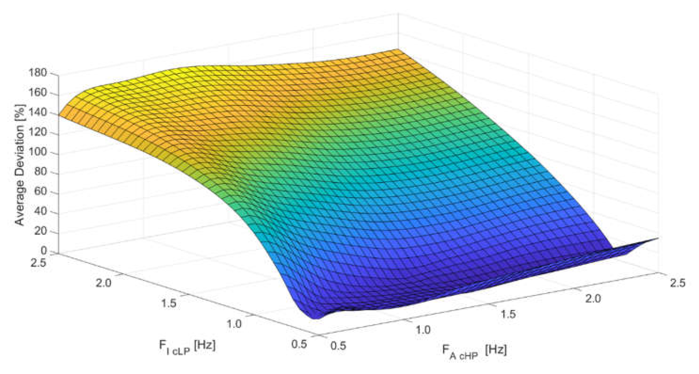
| High-pass filtration | --- | FA CHP = 1.67 Hz nAH = 6 |
| Low-pass filtration | FI CLP = 0.73 Hz nIL = 4 | FA CLP = 30 Hz nAL = 6 |
| Integration | cs = 1.01 | cd = 1.30 |
| Train | Root-Mean-Square Deviation | |||
|---|---|---|---|---|
| smin | smax | smin/dr min | smax/dr max | |
| [mm] | [mm] | [%] | [%] | |
| All trains | 0.64 | 0.53 | 4.8% | 8.2% |
| Multiple-unit trains ED250 | 0.41 | 0.54 | 3.8% | 7.5% |
| Separate locomotive EP09 and cars | 0.84 | 0.36 | 4.9% | 6.0% |
© 2020 by the authors. Licensee MDPI, Basel, Switzerland. This article is an open access article distributed under the terms and conditions of the Creative Commons Attribution (CC BY) license (http://creativecommons.org/licenses/by/4.0/).
Share and Cite
Olaszek, P.; Wyczałek, I.; Sala, D.; Kokot, M.; Świercz, A. Monitoring of the Static and Dynamic Displacements of Railway Bridges with the Use of Inertial Sensors. Sensors 2020, 20, 2767. https://doi.org/10.3390/s20102767
Olaszek P, Wyczałek I, Sala D, Kokot M, Świercz A. Monitoring of the Static and Dynamic Displacements of Railway Bridges with the Use of Inertial Sensors. Sensors. 2020; 20(10):2767. https://doi.org/10.3390/s20102767
Chicago/Turabian StyleOlaszek, Piotr, Ireneusz Wyczałek, Damian Sala, Marek Kokot, and Andrzej Świercz. 2020. "Monitoring of the Static and Dynamic Displacements of Railway Bridges with the Use of Inertial Sensors" Sensors 20, no. 10: 2767. https://doi.org/10.3390/s20102767
APA StyleOlaszek, P., Wyczałek, I., Sala, D., Kokot, M., & Świercz, A. (2020). Monitoring of the Static and Dynamic Displacements of Railway Bridges with the Use of Inertial Sensors. Sensors, 20(10), 2767. https://doi.org/10.3390/s20102767