A Variational Stacked Autoencoder with Harmony Search Optimizer for Valve Train Fault Diagnosis of Diesel Engine †


Abstract
1. Introduction
2. Theoretical Background
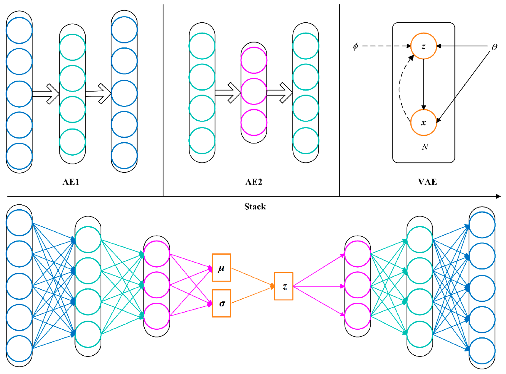
2.1. Variational Stacked Autoencoder
2.1.1. Autoencoder
2.1.2. Variational Autoencoder
2.1.3. VSAE Model
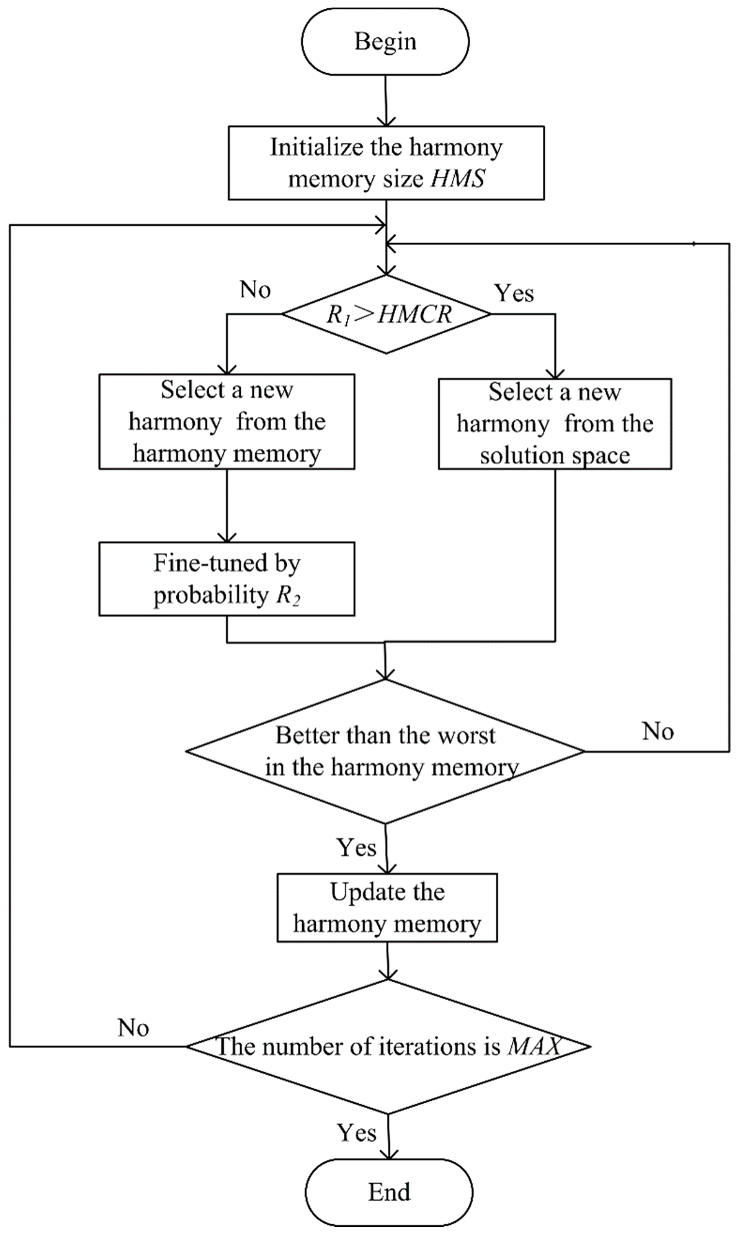
2.2. Harmony Search Optimizer
- Step 1: Define the objective function f(X), and initialize the harmony memory size HMS, the harmony memory considering rate HMCR, the pitch adjusting rate PCR, fine-tuning bandwidth B, and the maximum number of iterations MAX;
- Step 2: Determine the solution space, and randomly generate HMS group parameters from the solution space to form a harmony memory;
- Step 3: Randomly generate a variable R1 from [0, 1]. If R1 > HMCR, a new harmony is randomly selected from the solution space; otherwise, a new harmony is randomly selected from the harmony memory.
- Step 4: If the new harmony is generated in the harmony memory, a variable R2 is randomly generated from [0, 1] and compared with the PCR. If R1 > PCR, the harmony is not adjusted; otherwise, the harmony is fine-tuned bywhere Xnew is the adjusted harmony. R3 is a random number between [0, 1], and B is the adjustment bandwidth which is set to 2 in this paper.
- Step 5: If the resulting new harmony is better than the worst solution in the harmony memory, replace the worst harmony with the new harmony and update the harmony memory.
- Step 6: Repeat the above process until the number of iterations is MAX.
3. The Proposed HSO–VSAE Method
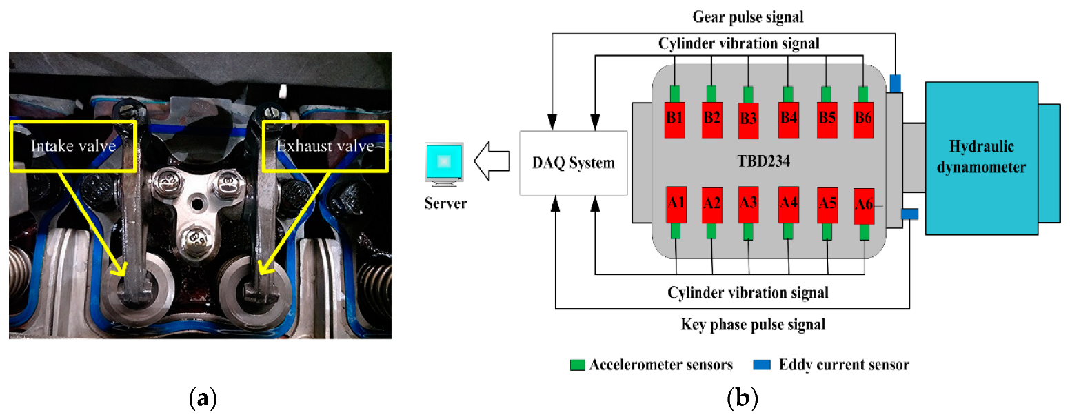
4. Test Rig and Data Description
5. Experimental Verification
5.1. Control Experiments
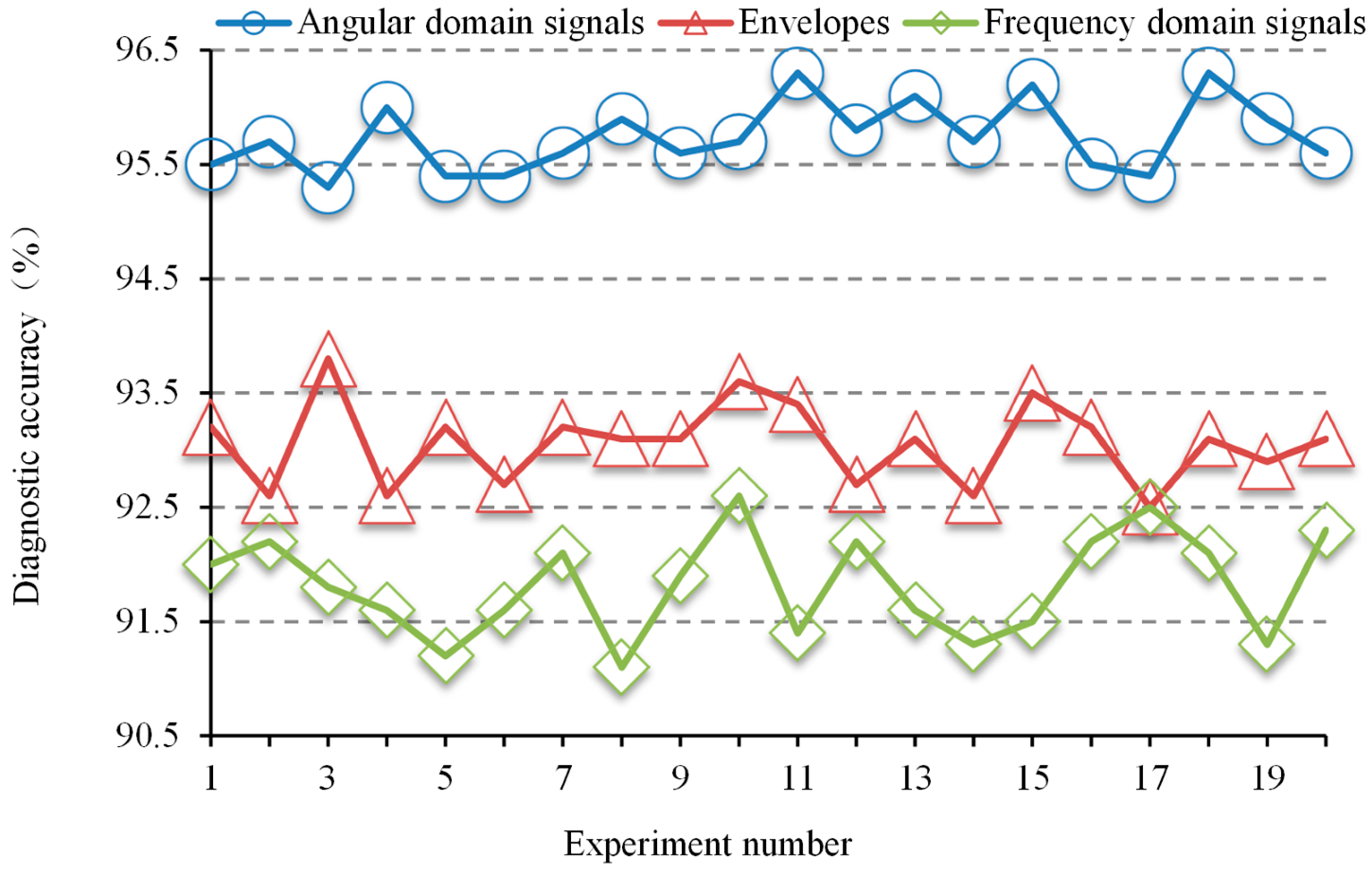
5.1.1. Model Input
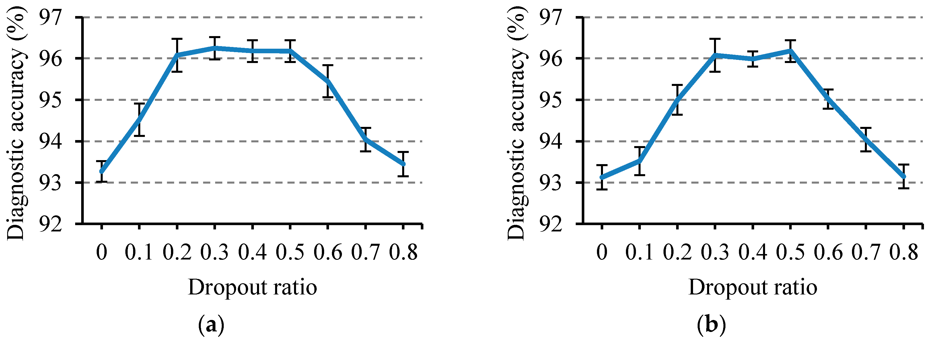
5.1.2. Dropout Rate
5.2. Parameter Optimization Based on HSO Algorithm
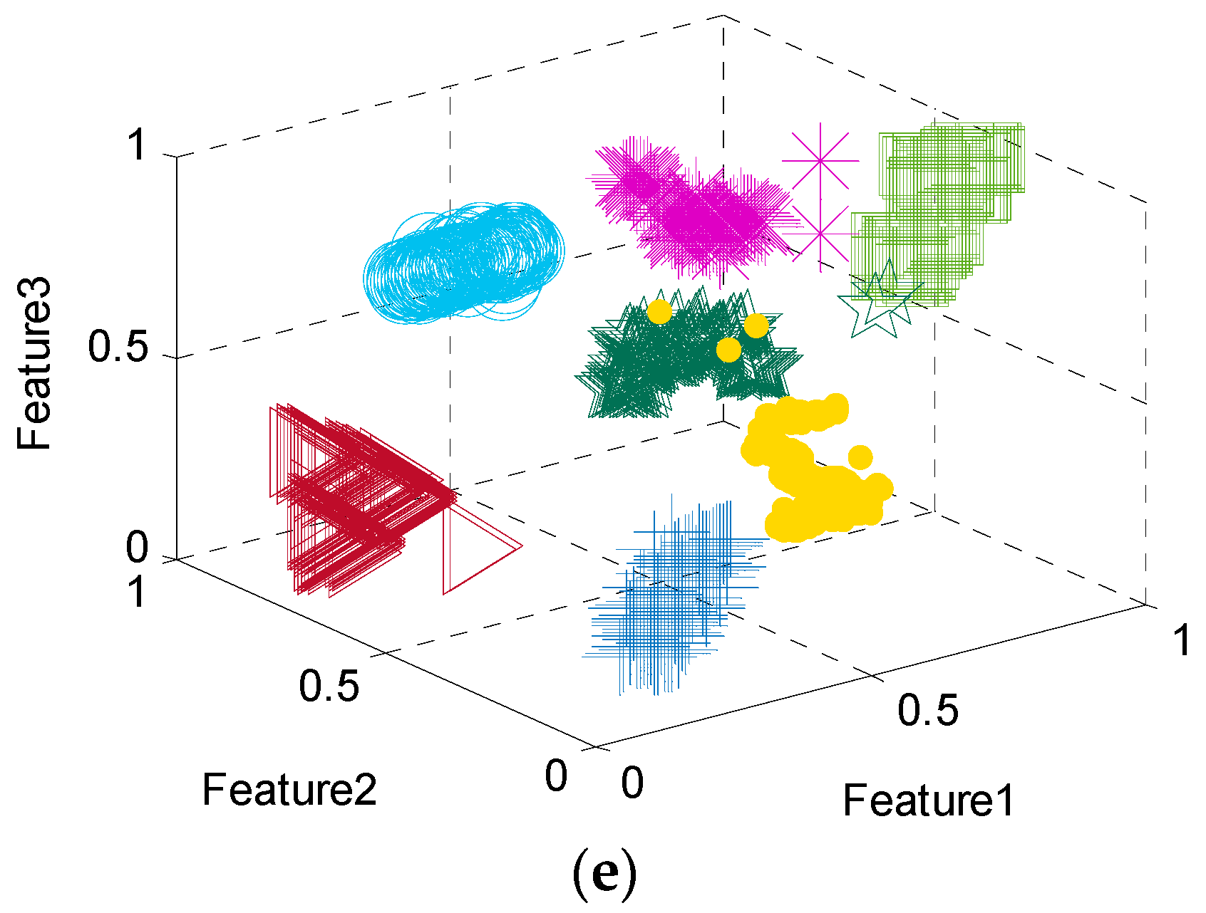
5.3. Feature Visualization
5.4. Analysis and Discussion of Diagnostic Results
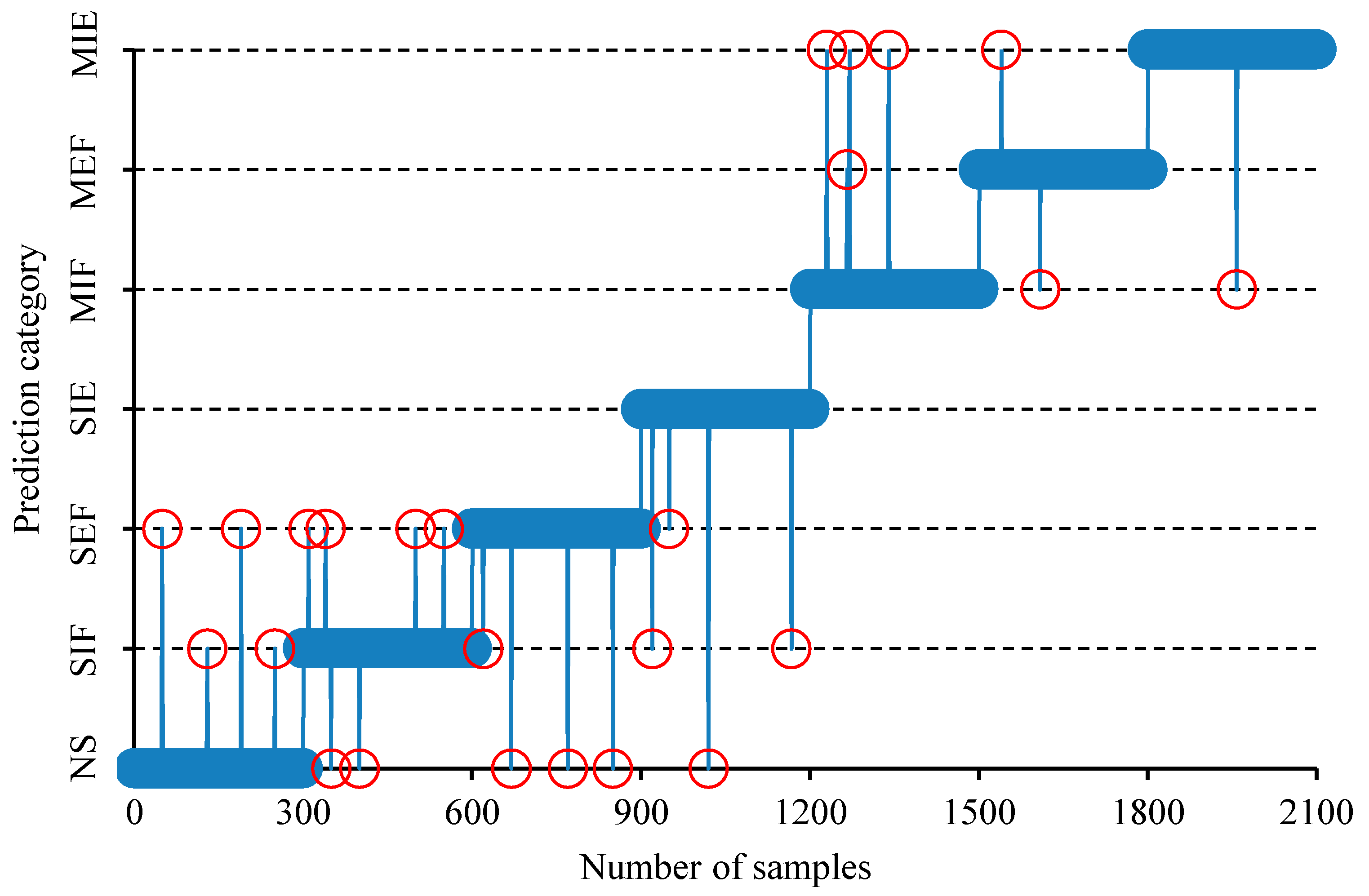
5.4.1. Detailed Analysis
5.4.2. Comparison with Baselines
6. Conclusions
Author Contributions
Funding
Conflicts of Interest
References
- Jiang, Z.N.; Mao, Z.W.; Wang, Z.J.; Zhang, J.J. Fault diagnosis of diesel engine valve clearance using the impact commencement detection method. Sensors 2017, 17, 2916. [Google Scholar] [CrossRef] [PubMed]
- Mao, Z.W.; Jiang, Z.N.; Zhao, H.P.; Zhang, J.J. Vibration-based fault diagnosis method for conrod small-end bearing knock in diesel engines. Insight 2018, 60, 418–425. [Google Scholar] [CrossRef]
- Zhao, H.P.; Zhang, J.J.; Jiang, Z.N.; Wei, D.H.; Zhang, X.D.; Mao, Z.W. A new fault diagnosis method for a diesel engine based on an optimized vibration Mel frequency under multiple operating conditions. Sensors 2019, 19, 2590. [Google Scholar] [CrossRef] [PubMed]
- Witek, L. Failure and thermo-mechanical stress analysis of the exhaust valve of diesel engine. Eng. Fail. Anal. 2016, 66, 154–165. [Google Scholar] [CrossRef]
- Ftoutou, E.; Chouchane, M.; Besbès, N. Diesel engine valve clearance fault classification using multivariate analysis of variance and discriminant analysis. Trans. Inst. Meas. Control 2012, 34, 566–577. [Google Scholar] [CrossRef]
- Flett, J.; Bone, G.M. Fault detection and diagnosis of diesel engine valve trains. Mech. Syst. Signal Process. 2016, 72, 316–327. [Google Scholar] [CrossRef]
- Li, Y.; Peter, W.T.; Yang, X.; Yang, J. EMD-based fault diagnosis for abnormal clearance between contacting components in a diesel engine. Mech. Syst. Signal Process. 2010, 24, 193–210. [Google Scholar] [CrossRef]
- Delvecchio, S.; Bonfiglio, P.; Pompoli, F. Vibro-acoustic condition monitoring of internal combustion engines: A critical review of existing techniques. Mech. Syst. Signal Process. 2018, 99, 661–683. [Google Scholar] [CrossRef]
- Ning, D.Y.; Sun, C.L.; Gong, Y.J.; Zhang, Z.M.; Hou, J.Y. Extraction of fault component from abnormal sound in diesel engines using acoustic signals. Mech. Syst. Signal Process. 2016, 75, 544–555. [Google Scholar]
- Wang, Q.; Zhang, P.L.; Meng, C.; Wang, H.G.; Wang, C. Extraction of fault component from abnormal sound in diesel engines using acoustic signals. Measurement 2019, 136, 625–635. [Google Scholar]
- Ahmad, T.A.; Alireza, M. Fault detection of injectors in diesel engines using vibration time-frequency analysis. Appl. Acoust. 2019, 143, 48–58. [Google Scholar]
- Yang, Y.S.; Ming, A.B.; Zhang, Y.Y.; Zhu, Y.S. Discriminative non-negative matrix factorization (DNMF) and its application to the fault diagnosis of diesel engine. Appl. Mech. Syst. Signal Process. 2017, 95, 158–171. [Google Scholar] [CrossRef]
- Moosavian, A.; Najafi, G.; Ghobadian, B.; Mirsalim, M. The effect of piston scratching fault on the vibration behavior of an IC engine. Appl. Acoust. 2017, 126, 91–100. [Google Scholar] [CrossRef]
- Yan, X.A.; Jia, M.P.; Zhao, Z.Z. A novel intelligent detection method for rolling bearing based on IVMD and instantaneous energy distribution-permutation entropy. Measurement 2018, 130, 435–447. [Google Scholar] [CrossRef]
- Hinton, G.E.; Osindero, S.; Teh, Y.W. A fast learning algorithm for deep belief nets. Neural Comput. 2006, 18, 1527–1554. [Google Scholar] [CrossRef] [PubMed]
- Ranzato, M.; Boureau, Y.L.; Lecun, Y. Sparse feature learning for deep belief networks. Adv. Neural Inf. Process. Syst. 2007, 20, 1185–1192. [Google Scholar]
- Muhammad, S.; Kim, C.H.; Kim, J.M. A hybrid feature model and deep-learning-based bearing fault diagnosis. Sensors 2017, 17, 2876. [Google Scholar]
- Liu, G.F.; Bao, H.Q.; Han, B.K. A stacked autoencoder-based deep neural network for achieving gearbox fault diagnosis. Math. Probl. Eng. 2018, 2018, 5105709. [Google Scholar] [CrossRef]
- Chen, Z.L.; Li, Z.N. Fault diagnosis method of rotating machinery based on stacked denoising autoencoder. J. Intell. Fuzzy Syst. 2018, 34, 3443–3449. [Google Scholar] [CrossRef]
- Meng, Z.; Zhan, X.Y.; Li, J.; Pan, Z.Z. An enhancement denoising autoencoder for rolling bearing fault diagnosis. Measurement 2018, 130, 448–454. [Google Scholar] [CrossRef]
- Lee, S.; Kwak, M.; Tsui, K.L.; Kim, S.B. Process monitoring using variational autoencoder for high-dimensional nonlinear processes. Eng. Appl. Artif. Intell. 2019, 83, 13–27. [Google Scholar] [CrossRef]
- Wang, K.; Forbes, M.G.; Gopaluni, B.; Chen, J.; Song, Z. Systematic development of a new variational autoencoder model based on uncertain data for monitoring nonlinear processes. IEEE Access 2019, 7, 22554–22565. [Google Scholar] [CrossRef]
- Zhang, Z.H.; Jiang, T.; Zhan, C.J.; Yang, Y.P. Gaussian feature learning based on variational autoencoder for improving nonlinear process monitoring. J. Process. Control. 2019, 75, 136–155. [Google Scholar] [CrossRef]
- Kingma, D.P.; Welling, M. Auto-encoding variational bayes. arXiv 2013, arXiv:1312.6114. [Google Scholar]
- Geem, Z.W.; Kim, J.H.; Loganathan, G.V. A new heuristic optimization algorithm: Harmony search. Simulation 2001, 76, 60–68. [Google Scholar] [CrossRef]
- Geem, Z.W. Novel derivative of harmony search algorithm for discrete design variables. Appl. Math. Comput. 2008, 199, 223–230. [Google Scholar] [CrossRef]
- Srivastava, N.; Hinton, G.E.; Krizhevsky, A.; Sutskever, I.; Salakhutdinov, R. Dropout: A simple way to prevent neural networks from overfitting. J. Mach. Learn. Res. 2014, 15, 1929–1958. [Google Scholar]
- Hinton, G.E.; Salakhutdinov, R.R. Reducing the dimensionality of data with neural networks. Science 2006, 313, 504–507. [Google Scholar] [CrossRef]
- Van Der Maaten, L.; Hinton, G. Visualizing data using t-SNE. J. Mach. Learn. Res. 2008, 9, 2579–2605. [Google Scholar]
- Chen, K.; Mao, Z.W.; Zhao, H.P.; Zhang, J.J. Valve fault diagnosis of internal combustion engine based on an improved stacked autoencoder. In Proceedings of the 2019 International Conference on Sensing, Diagnostics, Prognostics, and Control (SDPC), Beijing, China, 15–17 August 2019. [Google Scholar]


| Item | Value |
|---|---|
| Shape | V-shaped 60° |
| Number of cylinders | 12 |
| Compression ratio | 15:1 |
| Rating speed | 2100 r/min |
| Rating power | 485 kW |
| Firing sequence | B1-A1-B5-A5-B3-A3-B6-A6-B1-A2-B4-A4 |
| Fault Category | Intake Valve Clearance (mm) | Exhaust Valve Clearance (mm) | Number of Data Files |
|---|---|---|---|
| NS | 0.3 | 0.5 | 960 |
| SIF | 0.9 | 0.5 | 960 |
| SEF | 0.3 | 1.1 | 960 |
| SIE | 0.9 | 1.1 | 960 |
| MIF | 0.6 | 0.5 | 960 |
| MEF | 0.3 | 0.8 | 960 |
| MIE | 0.6 | 0.8 | 960 |
| Operating Condition | Speed (rpm) | Torque (N·m) |
|---|---|---|
| 1 | 1500 | 700 |
| 2 | 1500 | 1000 |
| 3 | 1500 | 1300 |
| 4 | 1800 | 700 |
| 5 | 1800 | 1000 |
| 6 | 1800 | 1300 |
| 7 | 1800 | 1600 |
| 8 | 2100 | 700 |
| 9 | 2100 | 1000 |
| 10 | 2100 | 1300 |
| 11 | 2100 | 1600 |
| 12 | 2100 | 2200 |
| Hyper-Parameter Combination | Dropout1 | Dropout2 | m | l | k | Accuracy (%) |
|---|---|---|---|---|---|---|
| 1 | 0.28 | 0.36 | 580 | 220 | 62 | 98.8 |
| 2 | 0.34 | 0.42 | 660 | 380 | 84 | 98.6 |
| 3 | 0.32 | 0.38 | 660 | 260 | 90 | 98.7 |
| 4 | 0.36 | 0.44 | 720 | 320 | 72 | 98.8 |
| 5 | 0.26 | 0.42 | 640 | 360 | 58 | 98.7 |
| 6 | 0.30 | 0.32 | 560 | 340 | 60 | 98.6 |
| 7 | 0.22 | 0.38 | 520 | 280 | 74 | 98.6 |
| Method | Average Accuracy ± Standard Deviation (%) | |||
|---|---|---|---|---|
| 20% Training Data Files | 40% Training Data Files | 60% Training Data Files | 80% Training Data Files | |
| KPCA + SVM | 85.29 ± 0.74 | 86.78 ± 0.71 | 88.43 ± 0.73 | 88.35 ± 0.77 |
| EEMD + KPCA + SVM | 92.13 ± 0.85 | 92.57 ± 0.82 | 93.16 ± 0.74 | 92.62 ± 0.69 |
| MLP | 88.43 ± 0.93 | 89.64 ± 0.87 | 90.65 ± 0.72 | 90.88 ± 0.70 |
| SAE | 93.20 ± 0.69 | 93.65 ± 0.62 | 94.10 ± 0.58 | 93.97 ± 0.53 |
| Proposed method | 97.23 ± 0.45 | 98.16 ± 0.37 | 98.85 ± 0.26 | 98.79 ± 0.31 |
| Method | Operating Condition | Accuracy (%) | |
|---|---|---|---|
| Training Set | Test Set | ||
| HSO-SAE | 4~12 | 1~3 | 93.4 |
| HSO-SAE | 1~3, 8~12 | 4~7 | 93.8 |
| HSO-SAE | 1~7 | 8~12 | 93.2 |
| HSO–VSAE | 4~12 | 1~3 | 98.4 |
| HSO–VSAE | 1~3, 8~12 | 4~7 | 98.6 |
| HSO–VSAE | 1~7 | 8~12 | 98.3 |
© 2019 by the authors. Licensee MDPI, Basel, Switzerland. This article is an open access article distributed under the terms and conditions of the Creative Commons Attribution (CC BY) license (http://creativecommons.org/licenses/by/4.0/).
Share and Cite
Chen, K.; Mao, Z.; Zhao, H.; Jiang, Z.; Zhang, J. A Variational Stacked Autoencoder with Harmony Search Optimizer for Valve Train Fault Diagnosis of Diesel Engine. Sensors 2020, 20, 223. https://doi.org/10.3390/s20010223
Chen K, Mao Z, Zhao H, Jiang Z, Zhang J. A Variational Stacked Autoencoder with Harmony Search Optimizer for Valve Train Fault Diagnosis of Diesel Engine. Sensors. 2020; 20(1):223. https://doi.org/10.3390/s20010223
Chicago/Turabian StyleChen, Kun, Zhiwei Mao, Haipeng Zhao, Zhinong Jiang, and Jinjie Zhang. 2020. "A Variational Stacked Autoencoder with Harmony Search Optimizer for Valve Train Fault Diagnosis of Diesel Engine" Sensors 20, no. 1: 223. https://doi.org/10.3390/s20010223
APA StyleChen, K., Mao, Z., Zhao, H., Jiang, Z., & Zhang, J. (2020). A Variational Stacked Autoencoder with Harmony Search Optimizer for Valve Train Fault Diagnosis of Diesel Engine. Sensors, 20(1), 223. https://doi.org/10.3390/s20010223