Large-Scale, Fine-Grained, Spatial, and Temporal Analysis, and Prediction of Mobile Phone Users’ Distributions Based upon a Convolution Long Short-Term Model

 ,
, 

Abstract
1. Introduction
2. Related Work
3. Data
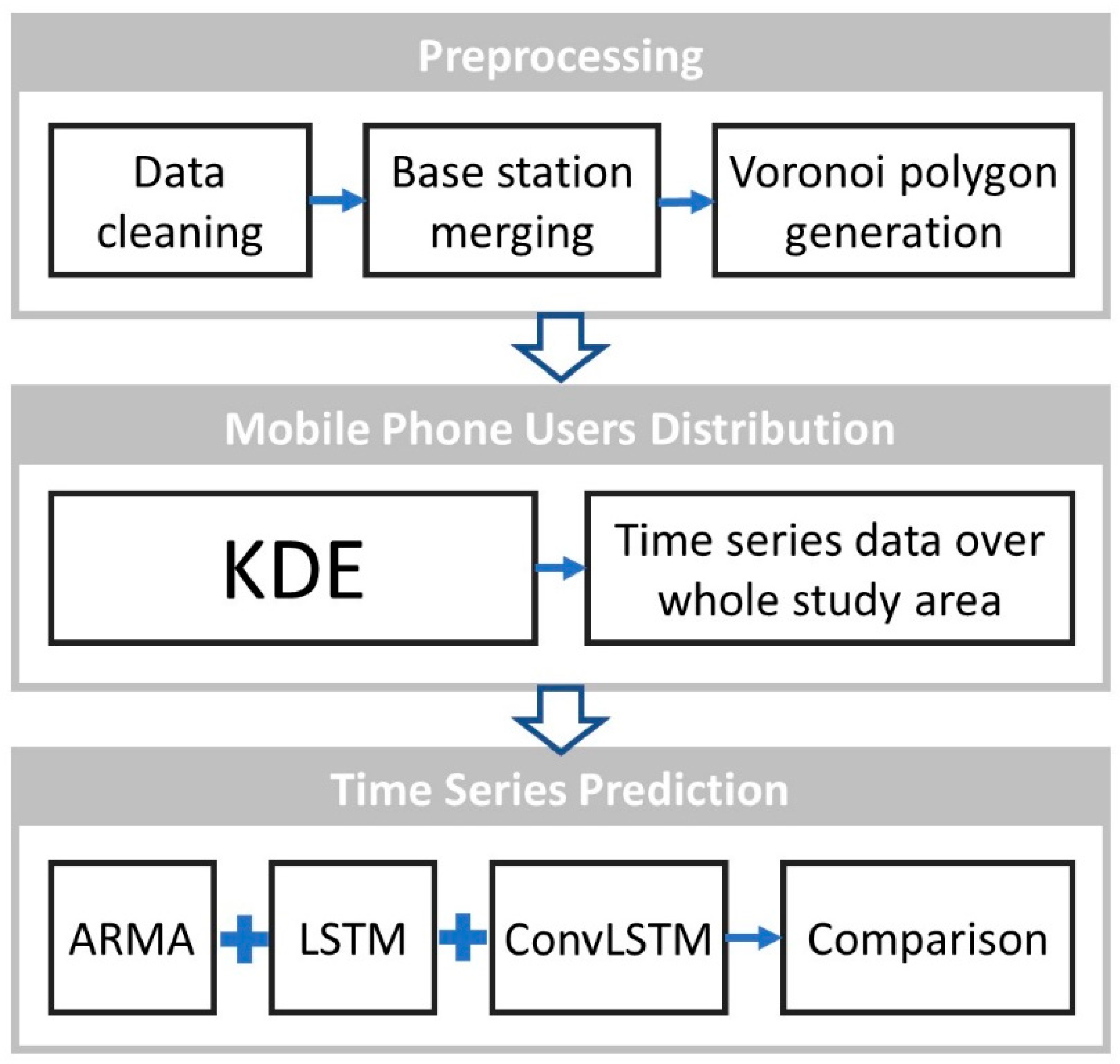
4. Method
4.1. Data Prepocessing
4.2. Modeling Mobile Users’ Population Distribution Using Kernel Density Estimation (KDE)
4.3. Prediction Models for Time-Series Data
4.3.1. ARMA Model
4.3.2. LSTM and Convolutional LSTM (ConvLSTM) Models
5. Results and Discussion
5.1. Determination of Mobile Users’ Population Distribution Using KDE
5.2. Prediction Results for the ConvLSTM Model
5.3. Prediction Results for the ConvLSTM Model versus the Two Baselines
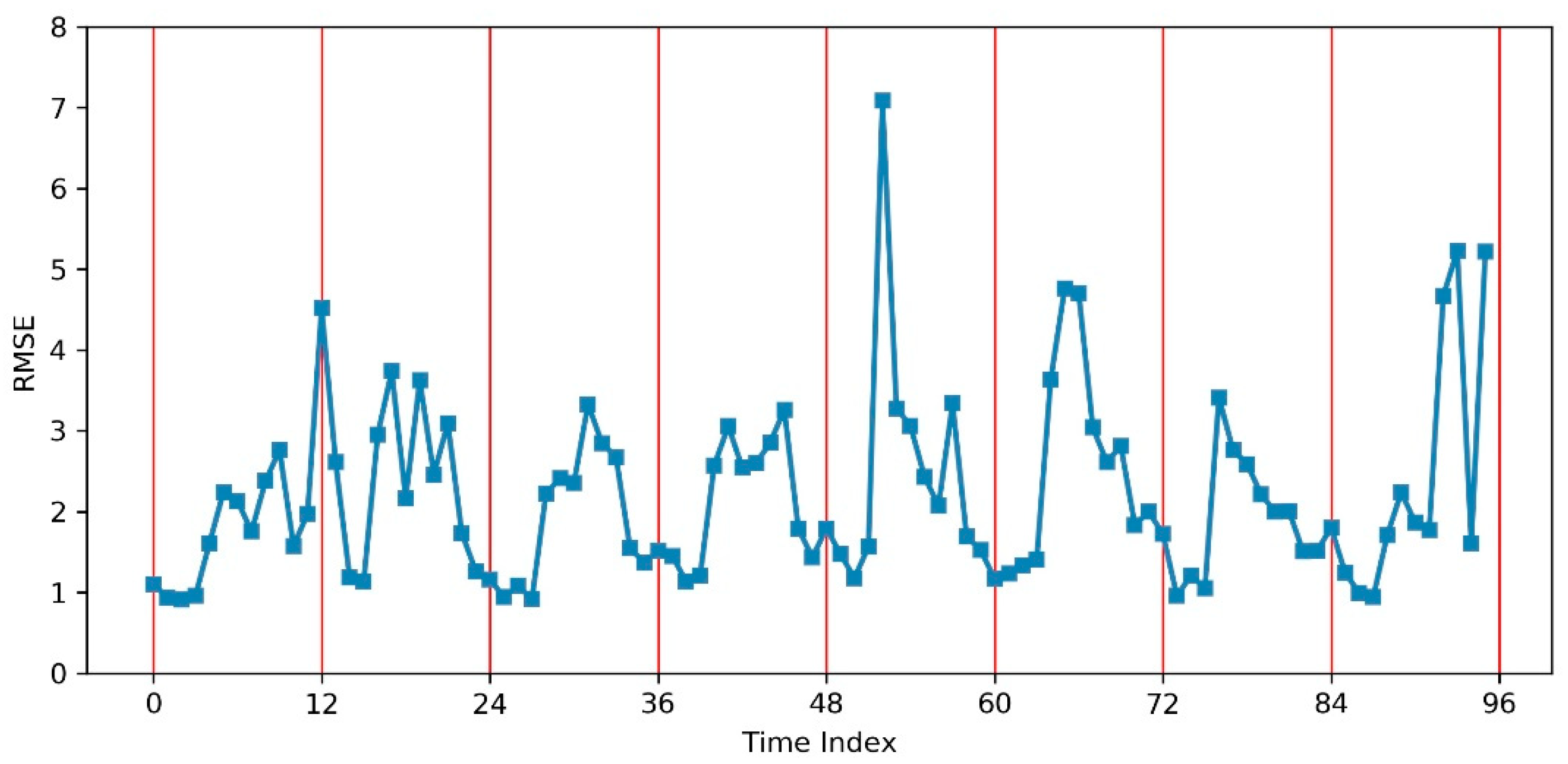
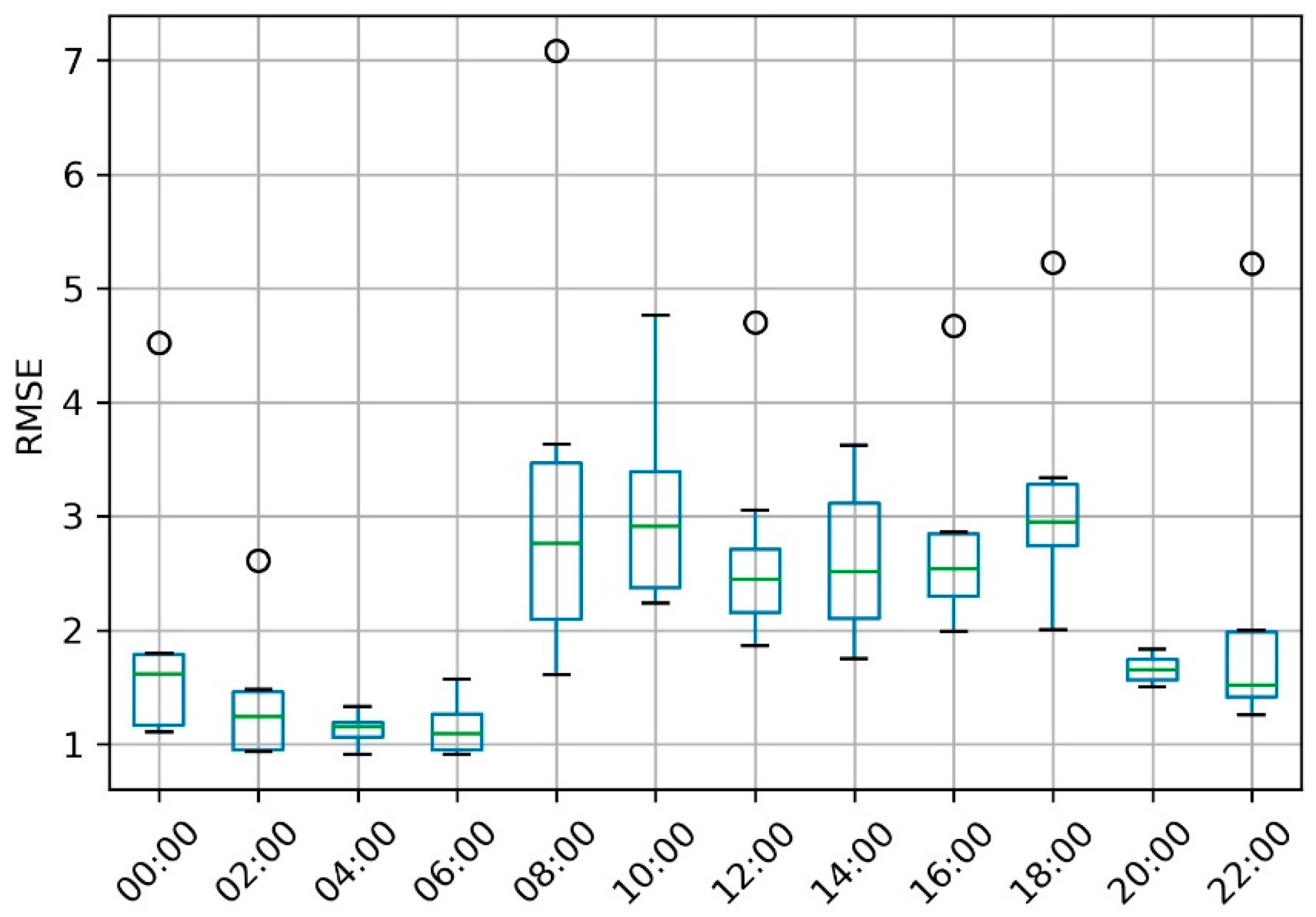
5.3.1. Results—Assessment of the Prediction Accuracy in Time
5.3.2. Results—Assessment of the Prediction Accuracy in Space
6. Conclusions
Author Contributions
Funding
Conflicts of Interest
References
- Becker, R.A.; Caceres, R.; Hanson, K.; Loh, J.M.; Urbanek, S.; Varshavsky, A.; Volinsky, C. A tale of one city: Using cellular network data for urban planning. IEEE Pervasive Comput. 2011, 10, 18–26. [Google Scholar] [CrossRef]
- De Nadai, M.; Staiano, J.; Larcher, R.; Sebe, N.; Quercia, D.; Lepri, B. The death and life of great Italian cities: A mobile phone data perspective. In Proceedings of the 25th International Conference on World Wide Web, Montréal, QC, Canada, 11–15 April 2016; pp. 413–423. [Google Scholar]
- Tao, S.; Corcoran, J.; Mateo-Babiano, I.; Rohde, D. Exploring Bus Rapid Transit passenger travel behaviour using big data. Appl. Geogr. 2014, 53, 90–104. [Google Scholar] [CrossRef]
- Li, Q.; Xu, B.; Ma, Y.; Chung, T. Real-time monitoring and forecast of active population density using mobile phone data. In Proceedings of the National Conference on Big Data Technology and Applications, Harbin, China, 25–26 December 2015; pp. 116–129. [Google Scholar]
- Traag, V.; Browet, A.; Calabrese, F.; Morlot, F. Social event detection in massive mobile phone data using probabilistic location inference. In Proceedings of the 2011 IEEE Third International Conference on Privacy, Security, Risk and Trust and 2011 IEEE Third International Conference on Social Computing, Boston, MA, USA, 9–11 October 2011. [Google Scholar]
- Zhou, J.; Pei, H.; Wu, H. Early Warning of Human Crowds Based on Query Data from Baidu Maps: Analysis Based on Shanghai Stampede. In Big Data Support of Urban Planning and Management; Springer: Berlin/Heidelberg, Germany, 2018; pp. 19–41. [Google Scholar]
- Bengtsson, L.; Lu, X.; Thorson, A.; Garfield, R.; Von Schreeb, J. Improved response to disasters and outbreaks by tracking population movements with mobile phone network data: A post-earthquake geospatial study in Haiti. PLoS Med. 2011, 8, e1001083. [Google Scholar] [CrossRef] [PubMed]
- Min, G.Y.; Jeong, D.H. Research on assessment of impact of big data attributes to disaster response decision-making process. J. Soc. E-Bus. Stud. 2013, 18. [Google Scholar] [CrossRef]
- Wilson, R.; Erbach-Schoenberg, E.; Albert, M.; Power, D.; Tudge, S.; Gonzalez, M.; Guthrie, S.; Chamberlain, H.; Brooks, C.; Hughes, C. Rapid and near real-time assessments of population displacement using mobile phone data following disasters: The 2015 Nepal Earthquake. PLoS Curr. 2016, 8. [Google Scholar] [CrossRef] [PubMed]
- Faria, N.R.; Rambaut, A.; Suchard, M.A.; Baele, G.; Bedford, T.; Ward, M.J.; Tatem, A.J.; Sousa, J.D.; Arinaminpathy, N.; Pépin, J. The early spread and epidemic ignition of HIV-1 in human populations. Science 2014, 346, 56–61. [Google Scholar] [CrossRef]
- Lopez, D.; Gunasekaran, M.; Murugan, B.S.; Kaur, H.; Abbas, K.M. Spatial big data analytics of influenza epidemic in Vellore, India. In Proceedings of the 2014 IEEE International Conference on Big Data (Big Data), Washington, DC, USA, 27–30 October 2014; pp. 19–24. [Google Scholar]
- Vespignani, A. Predicting the behavior of techno-social systems. Science 2009, 325, 425–428. [Google Scholar] [CrossRef]
- Liu, Z.; Ma, T.; Du, Y.; Pei, T.; Yi, J.; Peng, H. Mapping hourly dynamics of urban population using trajectories reconstructed from mobile phone records. Trans. GIS 2018, 22, 494–513. [Google Scholar] [CrossRef]
- Deville, P.; Linard, C.; Martin, S.; Gilbert, M.; Stevens, F.R.; Gaughan, A.E.; Blondel, V.D.; Tatem, A.J. Dynamic population mapping using mobile phone data. Proc. Natl. Acad. Sci. USA 2014, 111, 15888–15893. [Google Scholar] [CrossRef] [PubMed]
- Deng, L.; Xie, Y.; Huang, D. Bicycle-sharing facility planning base on riding spatio-temporal data. Planners 2017, 10, 82–88. [Google Scholar]
- Davis, B.; Lockwood, A.; Alcott, P.; Pantelidis, I.S. Food and Beverage Management; Routledge: London, UK, 2018. [Google Scholar]
- Mei, H.; Ma, A.; Poslad, S.; Oshin, T.O. Short-term traffic volume prediction for sustainable transportation in an urban area. J. Comput. Civ. Eng. 2013, 29, 04014036. [Google Scholar] [CrossRef]
- Kang, L.; Poslad, S.; Wang, W.; Li, X.; Zhang, Y.; Wang, C. A public transport bus as a flexible mobile smart environment sensing platform for IoT. In Proceedings of the 2016 12th International Conference on Intelligent Environments (IE), London, UK, 14–16 September 2016; pp. 1–8. [Google Scholar]
- Zhang, Z.; Poslad, S. A new post correction algorithm (PoCoA) for improved transportation mode recognition. In Proceedings of the 2013 IEEE International Conference on Systems, Man, and Cybernetics, Manchester, UK, 13–16 October 2013; pp. 1512–1518. [Google Scholar]
- Titkov, L.; Poslad, S.; Tan, J.J. An integrated approach to user-centered privacy for mobile information services. Appl. Artif. Intell. 2006, 20, 159–178. [Google Scholar] [CrossRef]
- Oshin, T.O.; Poslad, S.; Zhang, Z. Energy-efficient real-time human mobility state classification using smartphones. IEEE Trans. Comput. 2015, 64, 1680–1693. [Google Scholar] [CrossRef]
- Zheng, Y.; Zheng, W.; Xie, X. Collaborative Location and Activity Recommendations. U.S. Patent 8,719,198, 6 May 2014. [Google Scholar]
- Jiang, S.; Ferreira, J.; Gonzalez, M.C. Activity-based human mobility patterns inferred from mobile phone data: A case study of Singapore. IEEE Trans. Big Data 2017, 3, 208–219. [Google Scholar] [CrossRef]
- World Telecommunication Development Conference Dubai, United Arab Emirates. Available online: https://www.itu.int/en/ITU-D/Conferences/WTDC/Pages/default.aspxb (accessed on 7 May 2019).
- Blondel, V.D.; Decuyper, A.; Krings, G. A survey of results on mobile phone datasets analysis. EPJ Data Sci. 2015, 4, 10. [Google Scholar] [CrossRef]
- Kraemer, M.U.; Hay, S.I.; Pigott, D.M.; Smith, D.L.; Wint, G.W.; Golding, N. Progress and challenges in infectious disease cartography. Trends Parasitol. 2016, 32, 19–29. [Google Scholar] [CrossRef] [PubMed]
- Toole, J.L.; Lin, Y.-R.; Muehlegger, E.; Shoag, D.; González, M.C.; Lazer, D. Tracking employment shocks using mobile phone data. J. R. Soc. Interface 2015, 12. [Google Scholar] [CrossRef]
- Lu, X.; Wrathall, D.J.; Sundsøy, P.R.; Nadiruzzaman, M.; Wetter, E.; Iqbal, A.; Qureshi, T.; Tatem, A.; Canright, G.; Engø-Monsen, K. Unveiling hidden migration and mobility patterns in climate stressed regions: A longitudinal study of six million anonymous mobile phone users in Bangladesh. Glob. Environ. Chang. 2016, 38, 1–7. [Google Scholar] [CrossRef]
- Zhang, G.; Rui, X.; Fan, Y. Critical review of methods to estimate PM2.5 concentrations within specified research region. ISPRS Int. J. Geo-Inf. 2018, 7, 368. [Google Scholar] [CrossRef]
- Balk, D.; Yetman, G. The Global Distribution of Population: Evaluating the Gains in Resolution Refinement; Center for International Earth Science Information Network (CIESIN), Columbia University: New York, NY, USA, 2004. [Google Scholar]
- Bhaduri, B.; Bright, E.; Coleman, P.; Urban, M.L. LandScan USA: A high-resolution geospatial and temporal modeling approach for population distribution and dynamics. GeoJournal 2007, 69, 103–117. [Google Scholar] [CrossRef]
- Doxsey-Whitfield, E.; MacManus, K.; Adamo, S.B.; Pistolesi, L.; Squires, J.; Borkovska, O.; Baptista, S.R. Taking advantage of the improved availability of census data: A first look at the gridded population of the world, version 4. Pap. Appl. Geogr. 2015, 1, 226–234. [Google Scholar] [CrossRef]
- Lloyd, C.T.; Sorichetta, A.; Tatem, A.J. High resolution global gridded data for use in population studies. Sci. Data 2017, 4, 170001. [Google Scholar] [CrossRef]
- Department of International Economic and Social Affairs. Statistical Office. Principles and Recommendations for Population and Housing Censuses; revision 2; United Nations: New York, NY, USA, 2008. [Google Scholar]
- Lwin, K.K.; Sugiura, K.; Zettsu, K. Space-time multiple regression model for grid-based population estimation in urban areas. Int. J. Geogr. Inf. Sci. 2016, 30, 1579–1593. [Google Scholar] [CrossRef]
- Douglass, R.W.; Meyer, D.A.; Ram, M.; Rideout, D.; Song, D. High resolution population estimates from telecommunications data. EPJ Data Sci. 2015, 4, 4. [Google Scholar] [CrossRef]
- Kang, C.; Ma, X.; Tong, D.; Liu, Y. Intra-urban human mobility patterns: An urban morphology perspective. Phys. A: Stat. Mech. Its Appl. 2012, 391, 1702–1717. [Google Scholar] [CrossRef]
- Khodabandelou, G.; Gauthier, V.; El-Yacoubi, M.; Fiore, M. Population estimation from mobile network traffic metadata. In Proceedings of the 2016 IEEE 17th International Symposium on a World of Wireless, Mobile and Multimedia Networks (WoWMoM), Coimbra, Portugal, 21–24 June 2016; pp. 1–9. [Google Scholar]
- Gabrielli, L.; Furletti, B.; Trasarti, R.; Giannotti, F.; Pedreschi, D. City users’ classification with mobile phone data. In Proceedings of the 2015 IEEE International Conference on Big Data (Big Data), Santa Clara, CA, USA, 29 October–1 November 2015; pp. 1007–1012. [Google Scholar]
- Pappalardo, L.; Vanhoof, M.; Gabrielli, L.; Smoreda, Z.; Pedreschi, D.; Giannotti, F. An analytical framework to nowcast well-being using mobile phone data. Int. J. Data Sci. Anal. 2016, 2, 75–92. [Google Scholar] [CrossRef]
- Rojas, I.; Valenzuela, O.; Rojas, F.; Guillén, A.; Herrera, L.J.; Pomares, H.; Marquez, L.; Pasadas, M. Soft-computing techniques and ARMA model for time series prediction. Neurocomputing 2008, 71, 519–537. [Google Scholar] [CrossRef]
- Ji, W.; Chee, K.C. Prediction of hourly solar radiation using a novel hybrid model of ARMA and TDNN. Sol. Energy 2011, 85, 808–817. [Google Scholar] [CrossRef]
- Ling-ling, L.; Li, J.-H.; He, P.-J.; Wang, C.-S. The use of wavelet theory and ARMA model in wind speed prediction. In Proceedings of the 2011 1st International Conference on Electric Power Equipment-Switching Technology, Xi’an, China, 23–27 October 2011; pp. 395–398. [Google Scholar]
- Zhang, J.; Zheng, Y.; Qi, D.; Li, R.; Yi, X. DNN-based prediction model for spatio-temporal data. In Proceedings of the 24th ACM SIGSPATIAL International Conference on Advances in Geographic Information Systems, Burlingame, CA, USA, 31 October–3 November 2016; p. 92. [Google Scholar]
- Huang, W.; Song, G.; Hong, H.; Xie, K. Deep Architecture for Traffic Flow Prediction: Deep Belief Networks with Multitask Learning. IEEE Trans. Intell. Transp. Syst. 2014, 15, 2191–2201. [Google Scholar] [CrossRef]
- Polson, N.G.; Sokolov, V.O. Deep learning for short-term traffic flow prediction. Transp. Res. Part C Emerg. Technol. 2017, 79, 1–17. [Google Scholar] [CrossRef]
- Zhao, Z.; Chen, W.; Wu, X.; Chen, P.C.; Liu, J. LSTM network: A deep learning approach for short-term traffic forecast. IET Intell. Transp. Syst. 2017, 11, 68–75. [Google Scholar] [CrossRef]
- Qiu, M.; Zhao, P.; Zhang, K.; Huang, J.; Shi, X.; Wang, X.; Chu, W. A Short-Term Rainfall Prediction Model using Multi-Task Convolutional Neural Networks. In Proceedings of the 2017 IEEE International Conference on Data Mining (ICDM), New Orleans, LA, USA, 18–21 November 2017; pp. 395–404. [Google Scholar]
- Sutskever, I.; Vinyals, O.; Le, Q.V. Sequence to sequence learning with neural networks. In Proceedings of the Advances in Neural Information Processing Systems, Montreal, QC, Canada, 8–13 December 2014; pp. 3104–3112. [Google Scholar]
- Shi, X.; Chen, Z.; Wang, H.; Yeung, D.-Y.; Wong, W.-K.; Woo, W.-C. Convolutional LSTM network: A machine learning approach for precipitation nowcasting. In Proceedings of the Advances in Neural Information Processing Systems, Montreal, QC, Canada, 7–12 December 2015; pp. 802–810. [Google Scholar]
- Blumenstock, J.; Cadamuro, G.; On, R. Predicting poverty and wealth from mobile phone metadata. Science 2015, 350, 1073–1076. [Google Scholar] [CrossRef]
- Bogomolov, A.; Lepri, B.; Staiano, J.; Oliver, N.; Pianesi, F.; Pentland, A. Once upon a crime: Towards crime prediction from demographics and mobile data. In Proceedings of the 16th International Conference on Multimodal Interaction, Istanbul, Turkey, 12–16 November 2014; pp. 427–434. [Google Scholar]
- Zhao, R.; Yan, R.; Wang, J.; Mao, K. Learning to monitor machine health with convolutional bi-directional lstm networks. Sensors 2017, 17, 273. [Google Scholar] [CrossRef] [PubMed]
- Altché, F.; de La Fortelle, A. An LSTM network for highway trajectory prediction. In Proceedings of the 2017 IEEE 20th International Conference on Intelligent Transportation Systems (ITSC), Yokohama, Japan, 16–19 October 2017; pp. 353–359. [Google Scholar]
- Liu, T.; Bao, J.; Wang, J.; Zhang, Y. A Hybrid CNN–LSTM Algorithm for Online Defect Recognition of CO2 Welding. Sensors 2018, 18, 4369. [Google Scholar] [CrossRef]
- Rad, N.M.; Kia, S.M.; Zarbo, C.; Jurman, G.; Venuti, P.; Furlanello, C. Stereotypical motor movement detection in dynamic feature space. In Proceedings of the 2016 IEEE 16th International Conference on Data Mining Workshops (ICDMW), Barcelona, Spain, 12–15 December 2016; pp. 487–494. [Google Scholar]
- Liu, Y.; Zheng, H.; Feng, X.; Chen, Z. Short-term traffic flow prediction with Conv-LSTM. In Proceedings of the 2017 9th International Conference on Wireless Communications and Signal Processing (WCSP), Nanjing, China, 11–13 October 2017; pp. 1–6. [Google Scholar]
- Qiao, H.; Wang, T.; Wang, P.; Shibin, Q.; Lan, Z. A Time-Distributed Spatiotemporal Feature Learning Method for Machine Health Monitoring with Multi-Sensor Time Series. Sensors 2018, 18, 2932. [Google Scholar] [CrossRef]
- Yuan, Z.; Zhou, X.; Yang, T. Hetero-convlstm: A deep learning approach to traffic accident prediction on heterogeneous spatio-temporal data. In Proceedings of the 24th ACM SIGKDD International Conference on Knowledge Discovery & Data Mining, London, UK, 19–23 August 2018; pp. 984–992. [Google Scholar]
- Andrews, S.; Ellis, A.; Shaw, H.; Lukasz, P. Beyond self-report: Tools to compare estimated and real-world smartphone use. PLoS ONE 2015, 10, e0139004. [Google Scholar] [CrossRef]
- Brassel, K.E.; Reif, D. A procedure to generate Thiessen polygons. Geogr. Anal. 1979, 11, 289–303. [Google Scholar] [CrossRef]
- Rosenblatt, M. Remarks on some nonparametric estimates of a density function. Ann. Math. Stat. 1956, 832–837. [Google Scholar] [CrossRef]
- Parzen, E. On estimation of a probability density function and mode. Ann. Math. Stat. 1962, 33, 1065–1076. [Google Scholar] [CrossRef]
- Dehnad, K. Density Estimation for Statistics and Data Analysis; Taylor & Francis Group: Abingdon, UK, 1987. [Google Scholar]
- Fu, R.; Zhang, Z.; Li, L. Using LSTM and GRU neural network methods for traffic flow prediction. In Proceedings of the 2016 31st Youth Academic Annual Conference of Chinese Association of Automation (YAC), Wuhan, China, 11–13 November 2016; pp. 324–328. [Google Scholar]
- Chen, K.; Zhou, Y.; Dai, F. A LSTM-based method for stock returns prediction: A case study of China stock market. In Proceedings of the 2015 IEEE International Conference on Big Data (Big Data), Santa Clara, CA, USA, 29 October–1 November 2015; pp. 2823–2824. [Google Scholar]
- Gers, F.A.; Schmidhuber, J.; Cummins, F. Learning to forget: Continual prediction with LSTM. In Proceedings of the 1999 Ninth International Conference on Artificial Neural Networks ICANN 99. (Conf. Publ. No. 470), Edinburgh, UK, 7–10 September 1999. [Google Scholar]
- Boots, B.N.; Getis, A. Point Pattern Analysis; SAGE Publications, Incorporated: Beverly Hills, CA, USA, 1988; Volume 8. [Google Scholar]
- Kohavi, R. A study of cross-validation and bootstrap for accuracy estimation and model selection. IJCAI 1995, 14, 1137–1145. [Google Scholar]
- Bergmeir, C.; Benítez, M. On the use of cross-validation for time series predictor evaluation. Inf. Sci. 2012, 191, 192–213. [Google Scholar] [CrossRef]
- Kingma, D.P.; Ba, J. Adam: A method for stochastic optimization. arXiv 2014, arXiv:1412.6980. [Google Scholar]


| FID | Name | Description |
|---|---|---|
| 1 | Time | Interactive time of users and base station |
| 2 | CI | Corresponding base station ID |
| 3 | Tmsi | Encrypted ID of users |
| FID | Name | Description |
|---|---|---|
| 1 | CI | Unique ID of base station |
| 2 | Lon, Lat | Latitude and longitude of base station location |
| MAE | MSE | RMSE | |
|---|---|---|---|
| ConvLSTM | 0.816785 | 0.733462 | 0.835418 |
| LSTM | 0.891316 | 0.742480 | 0.887711 |
| ARMA | 0.859372 | 0.745777 | 0.858644 |
© 2019 by the authors. Licensee MDPI, Basel, Switzerland. This article is an open access article distributed under the terms and conditions of the Creative Commons Attribution (CC BY) license (http://creativecommons.org/licenses/by/4.0/).
Share and Cite
Zhang, G.; Rui, X.; Poslad, S.; Song, X.; Fan, Y.; Ma, Z. Large-Scale, Fine-Grained, Spatial, and Temporal Analysis, and Prediction of Mobile Phone Users’ Distributions Based upon a Convolution Long Short-Term Model. Sensors 2019, 19, 2156. https://doi.org/10.3390/s19092156
Zhang G, Rui X, Poslad S, Song X, Fan Y, Ma Z. Large-Scale, Fine-Grained, Spatial, and Temporal Analysis, and Prediction of Mobile Phone Users’ Distributions Based upon a Convolution Long Short-Term Model. Sensors. 2019; 19(9):2156. https://doi.org/10.3390/s19092156
Chicago/Turabian StyleZhang, Guangyuan, Xiaoping Rui, Stefan Poslad, Xianfeng Song, Yonglei Fan, and Zixiang Ma. 2019. "Large-Scale, Fine-Grained, Spatial, and Temporal Analysis, and Prediction of Mobile Phone Users’ Distributions Based upon a Convolution Long Short-Term Model" Sensors 19, no. 9: 2156. https://doi.org/10.3390/s19092156
APA StyleZhang, G., Rui, X., Poslad, S., Song, X., Fan, Y., & Ma, Z. (2019). Large-Scale, Fine-Grained, Spatial, and Temporal Analysis, and Prediction of Mobile Phone Users’ Distributions Based upon a Convolution Long Short-Term Model. Sensors, 19(9), 2156. https://doi.org/10.3390/s19092156