A Novel Method for Classifying Liver and Brain Tumors Using Convolutional Neural Networks, Discrete Wavelet Transform and Long Short-Term Memory Networks


Abstract
1. Introduction
2. Related Works
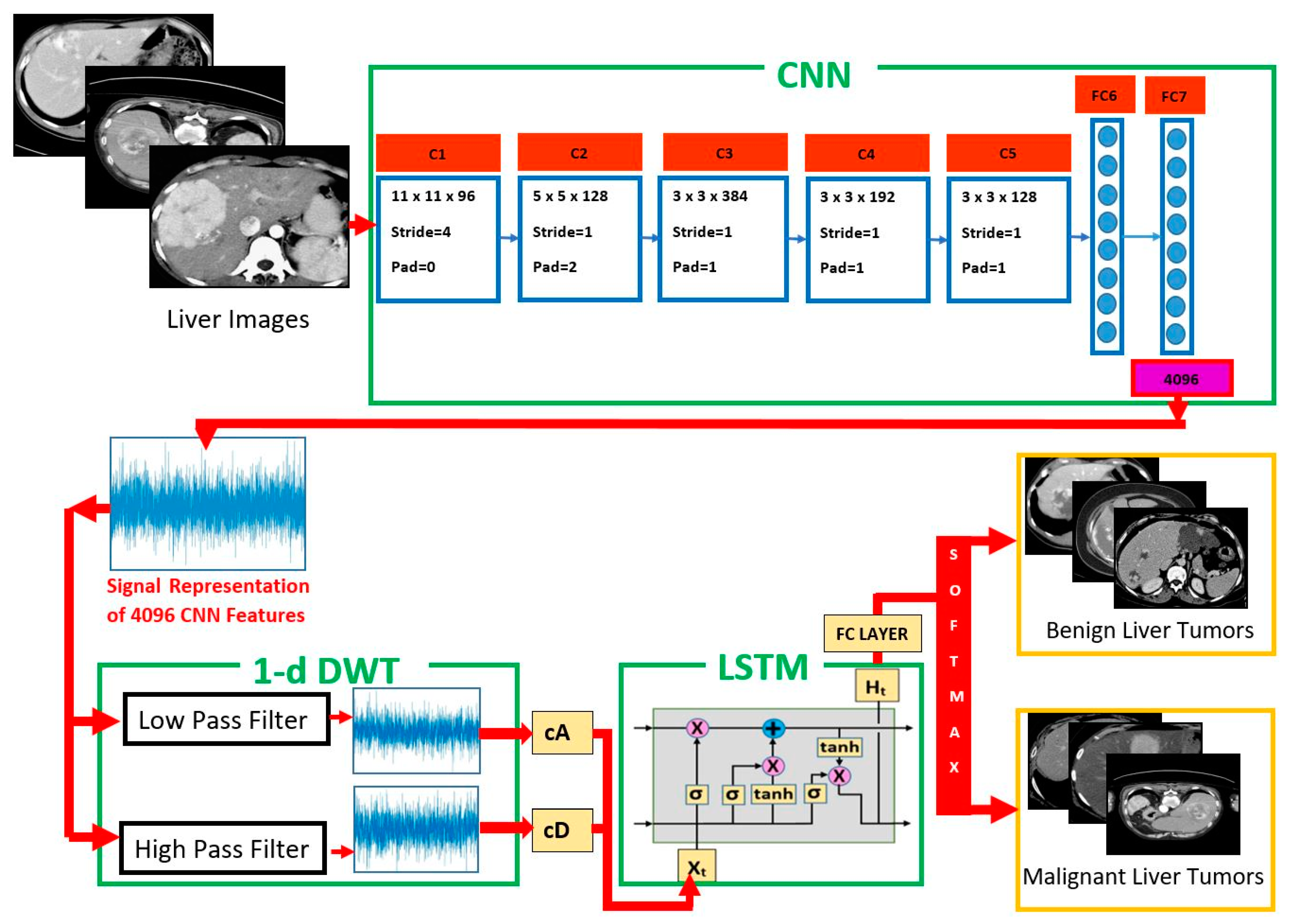
3. Proposed CNN–DWT–LSTM Method
3.1. Pre-Trained AlexNet CNN Architecture for Feature Extraction
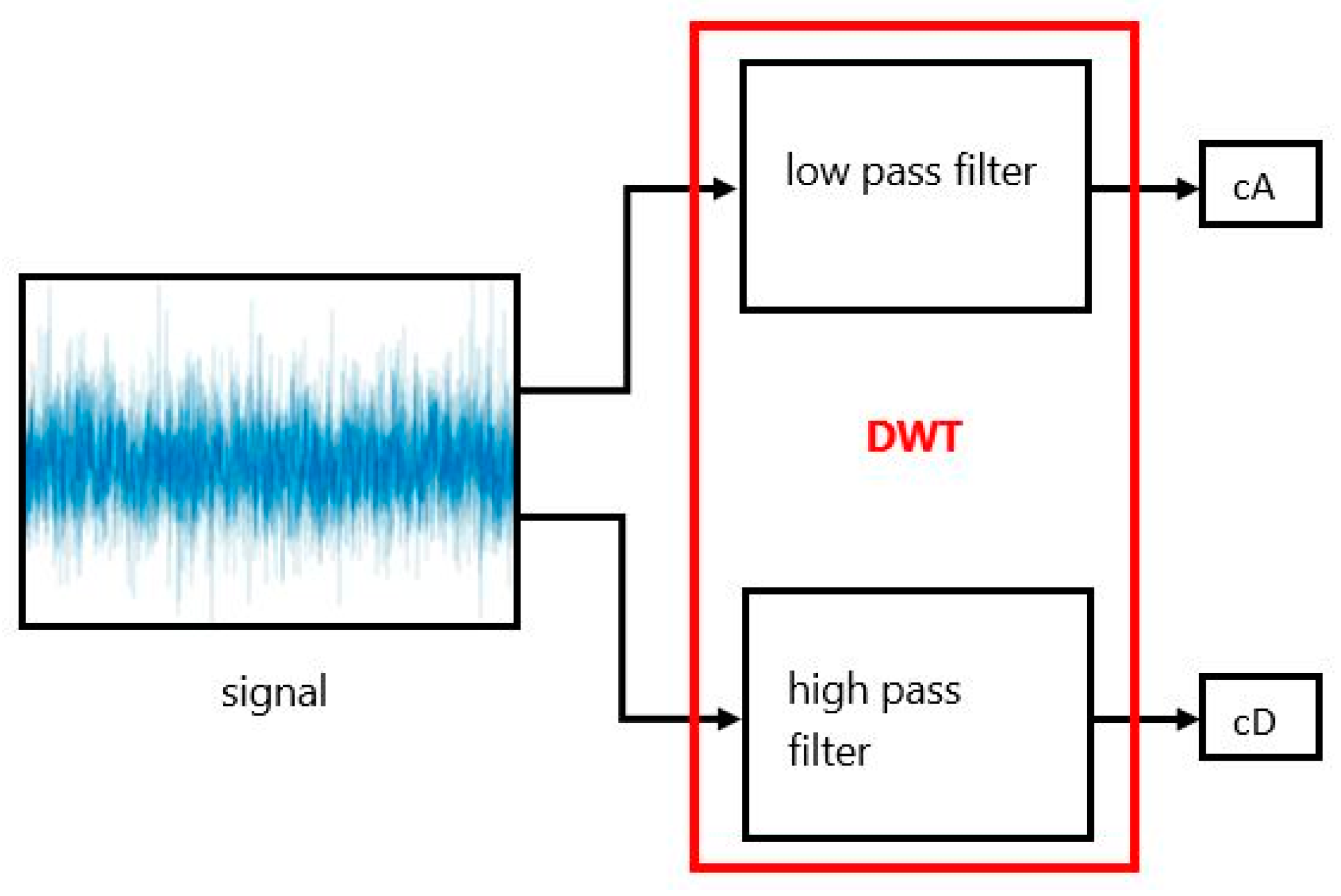
3.2. DWT as Feature Extraction and Reduction of Feature Vector Dimension
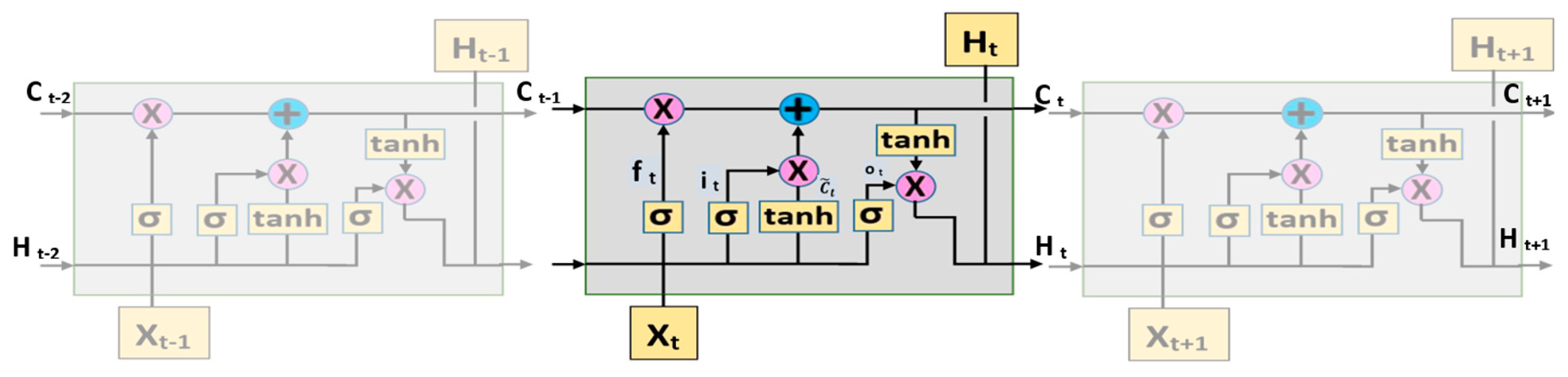
3.3. LSTM-Based Image Classification
4. Experimental Results
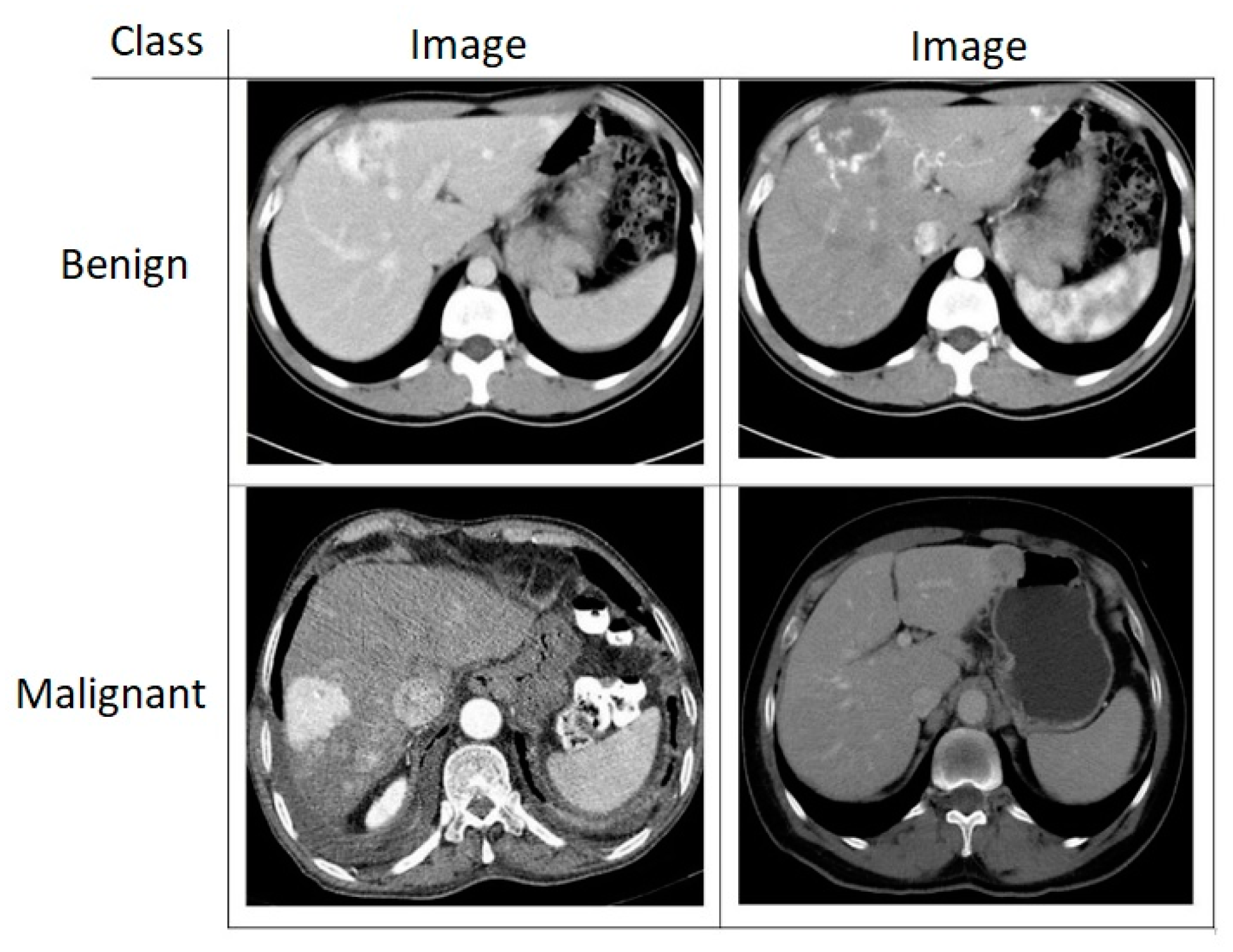
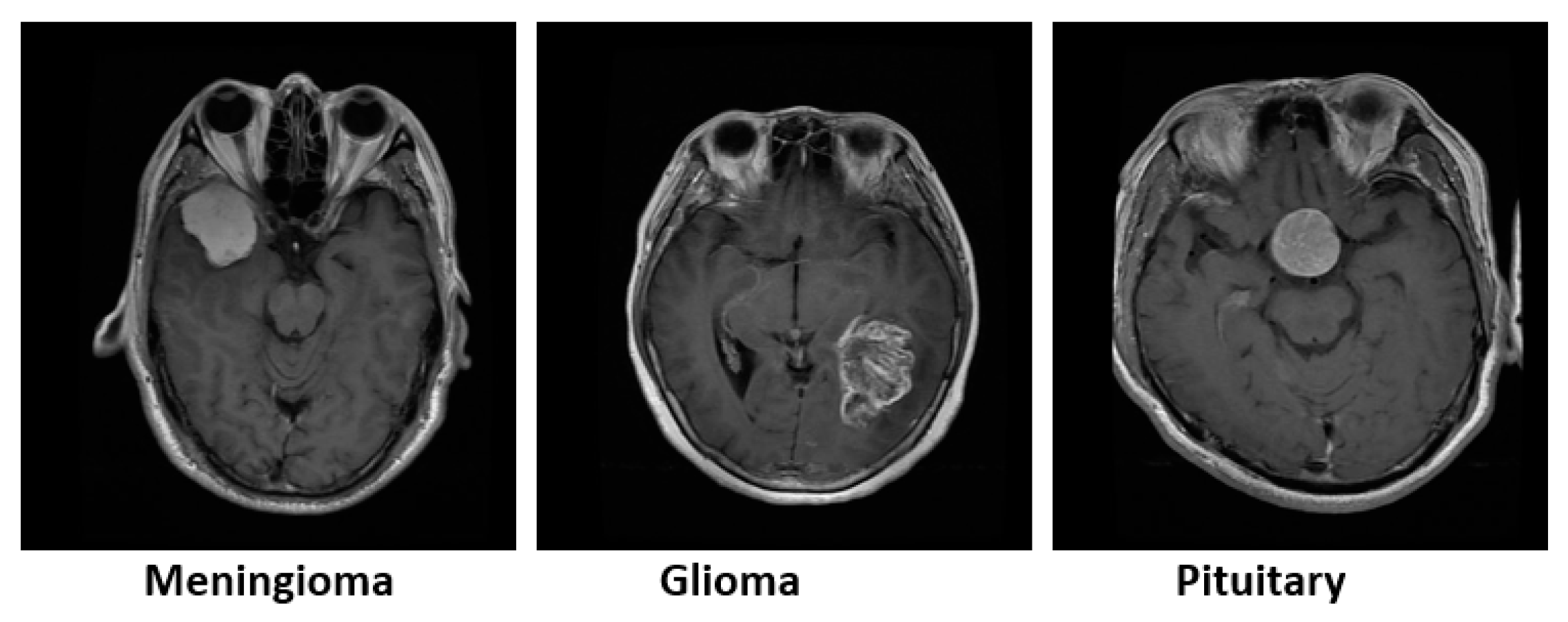
4.1. Dataset
4.2. Experimental Tools
4.3. Classifier Comparisons
4.4. Performance Measurements
4.5. Classification Performance
4.6. Discussion
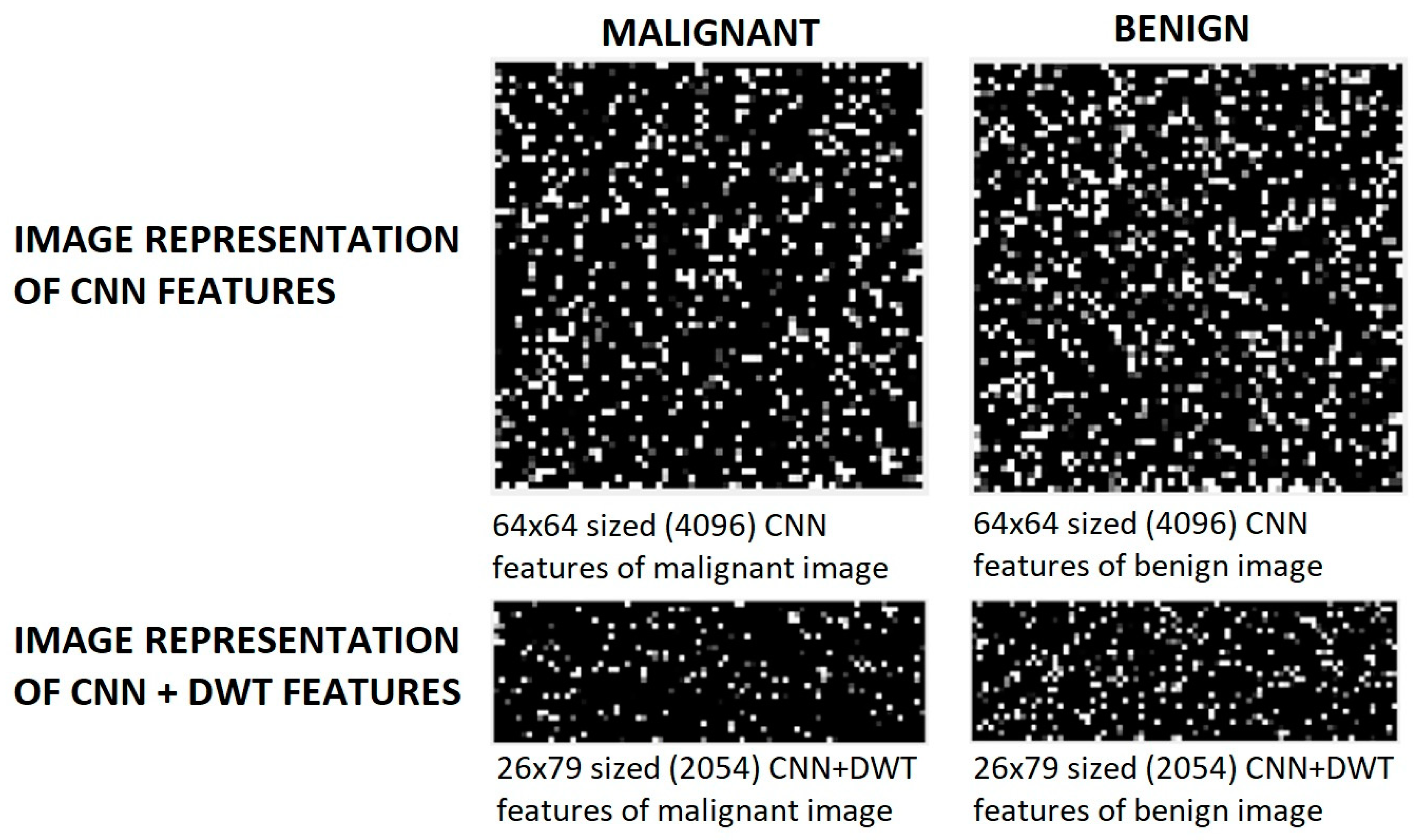
- Taking advantage of CNN’s success in feature extraction and obtaining a feature vector of 1 × 4096.
- Considering the 1 × 4096 feature vector as a signal and separating the signal into low-frequency components by utilizing the success of 1-D DWT in dimension reduction, feature extraction, and detect signal discontinuities.
- Taking advantage of the success of the LSTM structure in signal classification and obtaining a new robust image classifier.
- Experimental results show that the study reached its goals.
5. Conclusions
Author Contributions
Funding
Acknowledgments
Conflicts of Interest
References
- Kaya, H.; Çavuşoğlu, A.; Çakmak, H.B.; Şen, B.; Delen, D. Image segmentation and image simulation methods with the help of the diagnosis and treatment of post-treatment processes: Keratoconus example. J. Fac. Eng. Archit. Gazi Univ. 2016, 31, 737–747. [Google Scholar] [CrossRef][Green Version]
- Wu, K.; Chen, X.; Ding, M. Deep learning based classification of focal liver lesions with contrast-enhanced ultrasound. Optik-Int. J. Light Electron Opt. 2014, 125, 4057–4063. [Google Scholar] [CrossRef]
- Jabarulla, M.Y.; Lee, H.N. Computer aided diagnostic system for ultrasound liver images: A systematic review. Optik-Int. J. Light Electron Opt. 2017, 140, 1114–1126. [Google Scholar] [CrossRef]
- Alahmer, H.; Ahmed, A. Computer-aided classification of liver lesions from CT images based on multiple ROI. Procedia Comput. Sci. 2016, 90, 80–86. [Google Scholar] [CrossRef]
- Kumar, S.S.; Moni, R.S.; Rajeesh, J. Liver tumor diagnosis by gray level and contourlet coefficients texture analysis. In Proceedings of the 2012 International Conference on Computing, Electronics and Electrical Technologies (ICCEET), Kumaracoil, India, 21–22 March 2012; pp. 557–562. [Google Scholar] [CrossRef]
- Jakimovski, G.; Danco, D. Using Double Convolution Neural Network for Lung Cancer Stage Detection. Appl. Sci. 2019, 9, 427. [Google Scholar] [CrossRef]
- Yoo, Y.; Baek, J. A Novel Image Feature for the Remaining Useful Lifetime Prediction of Bearings Based on Continuous Wavelet Transform and Convolutional Neural Network. Appl. Sci. 2018, 8, 1102. [Google Scholar] [CrossRef]
- Doğantekin, A.; Özyurt, F.; Avcı, E.; Koç, M. A novel approach for liver image classification: PH-C-ELM. Measurement 2019, 37, 332–338. [Google Scholar] [CrossRef]
- Lipton, Z.C. A Critical Review of Recurrent Neural Networks for Sequence Learning. arXiv 2015, arXiv:1506.00019. [Google Scholar]
- Chen, J.L.; Wang, Y.L.; Wu, Y.; Cai, C.Q. An Ensemble of Convolutional Neural Networks for Image Classification Based on LSTM. In Proceedings of the 2017 International Conference on Green Informatics (ICGI), Fuzhou, China, 15–17 August 2017. [Google Scholar] [CrossRef]
- Shahzadi, I.; Tang, T.B.; Meriadeau, F.; Quyyum, A. CNN-LSTM: Cascaded Framework For Brain Tumour Classification. In Proceedings of the 2018 IEEE-EMBS Conference on Biomedical Engineering and Sciences (IECBES), Sarawak, Malaysia, 3–6 December 2018. [Google Scholar] [CrossRef]
- Rachmadi, R.F.; Uchimura, K.; Koutaki, G.; Ogata, K. Single image vehicle classification using pseudo long short-term memory classifier. J. Vis. Commun. Image Represent. 2018, 56, 265–274. [Google Scholar] [CrossRef]
- An, F.; Liu, Z. Facial expression recognition algorithm based on parameter adaptive initialization of CNN and LSTM. Vis. Comput. 2019, 12, 1–16. [Google Scholar] [CrossRef]
- Guo, Y.; Liu, Y.; Bakker, E.M.; Guo, Y.; Lew, Y.S. CNN-RNN: A large-scale hierarchical image classification framework. Multimed. Tools Appl. 2018, 77, 10251–10271. [Google Scholar] [CrossRef]
- Lakhal, M.I.; Çevikalp, H.; Escalera, S.; Ofli, F. Recurrent neural networks for remote sensing image classification. IET Comput. Vis. 2018, 12, 1040–1045. [Google Scholar] [CrossRef]
- Zuo, Z.; Shuai, B.; Wang, G.; Liu, X.; Wang, X.; Wang, B.; Chen, Y. Convolutional recurrent neural networks: Learning spatial dependencies for image representation. In Proceedings of the 2015 IEEE Conference on Computer Vision and Pattern Recognition Workshops (CVPRW), Boston, MA, USA, 7–12 June 2015. [Google Scholar] [CrossRef]
- Liu, Y. Wavelet feature extraction for high-dimensional microarray data. Neurocomputing 2009, 72, 4–6. [Google Scholar] [CrossRef]
- Khatami, A.; Khasravi, A.; Nguyen, T.; Lim, C.P.; Nahavandi, S. Medical image analysis using wavelet transform and deep belief networks. Expert Syst. Appl. 2017, 86, 190–198. [Google Scholar] [CrossRef]
- Yadav, A.R.; Anand, R.S.; Deval, M.L.; Gupta, S. Hardwood species classification with DWT based hybrid texture feature extraction techniques. Sadhana 2015, 40, 8–2287. [Google Scholar] [CrossRef]
- Vogiatzis, D.; Tsapatsoulis, N. Active learning with wavelets for microarray data. Lect. Notes Comput. Sci. 2006, 3849, 252–258. [Google Scholar] [CrossRef][Green Version]
- Wang, X.H.; Istepanian, R.S.H.; Song, Y.H. Application of wavelet modulus maxima in microarray spots recognition. IEEE Trans. Nano Biosci. 2003, 2, 190–192. [Google Scholar] [CrossRef]
- Wang, J.; Jennie, Z.; Ma, J.; Li, M. Normalization of cDNA microarray data using wavelet regressions. Comb. Chem. High Throughput Screen. 2004, 7, 783–791. [Google Scholar] [CrossRef]
- Klevecz, R. Dynamic architecture of the yeast cell cycle uncovered wavelet decomposition of expression microarray data. Funct. Integr. Genom. 2000, 1, 186–192. [Google Scholar] [CrossRef]
- Bennet, J.; Ganaprakasam, C.A.; Arputharaj, K. A Discrete Wavelet Based Feature Extraction and Hybrid Classification Technique for Microarray Data Analysis. Sci. World J. 2014, 2014, 195470. [Google Scholar] [CrossRef]
- Bishop, C.M. Neural Networks for Pattern Recognition; Oxford University Press: New York, NY, USA, 1995. [Google Scholar]
- Morocho, V.; Vanegas, P.; Medina, R. Hepatic steatosis detection using the Co-occurrence matrix in tomography and ultrasound images. In Proceedings of the 20th Symposium on Signal Processing, Images and Computer Vision (STSIVA), Bogota, Colombia, 2–4 September 2015; pp. 1–7. [Google Scholar] [CrossRef]
- Wu, J.Y.; Beland, M.; Konrad, J.; Tuomi, A.; Glidden, D.; Grand, D.; Merck, D. Quantitative ultrasound texture analysis for clinical decision making support. Med. Imaging Ultrason. Imaging Tomogr. 2015, 9419, 94190W. [Google Scholar]
- Hwang, Y.N.; Lee, J.H.; Kim, G.Y.; Jiang, Y.Y.; Kim, S.M. Classification of focal liver lesions on ultrasound images by extracting hybrid textural features and using an artificial neural network. Bio-Med. Mater. Eng. 2015, 26, S1599–S1611. [Google Scholar] [CrossRef] [PubMed]
- Acharya, U.R.; Fujita, H.; Bhat, S.; Raghavendra, U.; Gudigar, A.; Molinari, F.; Vijayananthan, A.; Ng, K.H. Decision support system for fatty liver disease using GIST descriptors extracted from ultrasound images. Inf. Fusion 2016, 29, 32–39. [Google Scholar] [CrossRef]
- Özyurt, F.; Tuncer, T.; Avci, E. A Novel Liver Image Classification Method Using Perceptual Hash-Based Convolutional Neural Network. Arab. J. Sci. Eng. 2019, 44, 3173–3182. [Google Scholar] [CrossRef]
- Cheng, J.; Huang, W.; Cao, S.; Yang, R.; Yang, W.; Yun, Z.; Wang, Z.; Feng, Q. Enhanced Performance of Brain Tumor Classification via Tumor Region Augmentation and Partition. PLoS ONE 2015, 10, e0140381. [Google Scholar] [CrossRef] [PubMed]
- Cheng, J. Brain Tumor Dataset. Available online: https://figshare.com/articles/brain_tumor_dataset/1512427 (accessed on 1 January 2019).
- Cheng, J.; Yang, W.; Huang, M.; Huang, W.; Jiang, J.; Zhou, Y.; Yang, R.; Zhao, J.; Feng, Q.; Chen, W. Retrieval of Brain Tumors by Adaptive Spatial Pooling and Fisher Vector Representation. PLoS ONE 2016, 11, e0157112. [Google Scholar] [CrossRef] [PubMed]
- Paul, S.J.; Plassard, A.J.; Landman, B.A.; Fabbri, D. Deep Learning for Brain Tumor Classification. SPIE Proc. 2017, 10137, 1013710. [Google Scholar] [CrossRef]
- Abiwinanda, N.; Hanif, M.; Hesaputra, S.T.; Handayani, A.; Mengko, T.R. Brain Tumor Classification Using Convolutional Neural Network. In Proceedings of the World Congress on Medical Physics and Biomedical Engineering, Prague, Czech Republic, 3–8 June 2018; pp. 183–189. [Google Scholar] [CrossRef]
- Menezes, J.; Poojary, N. Dimensionality Reduction and Classification of Hyperspetral Images using DWT and DCCF. In Proceedings of the 2016 3rd MEC International Conference on Big Data and Smart City (ICBDSC), Muscat, Oman, 15–16 March 2016. [Google Scholar] [CrossRef]
- Ara, S.R.; Bashar, S.K.; Alam, F.; Hasan, M.K. EMD-DWT based transform domain feature reduction approach for quantitative multi-class classification of breast lesions. Ultrasonics 2017, 80, 22–33. [Google Scholar] [CrossRef]
- Kaya, A.; Keceli, A.S.; Catal, C.; Yalic, H.Y.; Temucin, H.; Tekinerdoğan, B. Analysis of transfer learning for deep neural network based plant classification models. Comput. Electron. Agric. 2019, 158, 20–29. [Google Scholar] [CrossRef]
- Shin, H.C.; Roth, H.R.; Gao, M.; Lu, L.; Xu, Z.; Nogues, I.; Yao, J.; Mollura, D.; Summers, R.M. Deep convolutional neural networks for computer-aided detection: Cnn architectures, dataset characteristics and transfer learning. IEEE Trans. Med. Imaging 2016, 35, 1285–1298. [Google Scholar] [CrossRef]
- Williams, T.; Li, R. Wavelet Pooling for Convolutional Neural Networks. In Proceedings of the International Conference on Learning Representations (ICLR), Vancouver, BC, Canada, 30 April–3 May 2018. [Google Scholar]
- Fujieda, S.; Takayama, K.; Hachisuka, T. Wavelet Convolutional Neural Networks. arxiv 2018, arXiv:1805.08620. [Google Scholar]
- Fujieda, S.; Takayama, K.; Hachisuka, T. Wavelet Convolutional Neural Networks for Texture Classification. arxiv 2017, arXiv:1707.07394. [Google Scholar]
- Agarap, A.F.M. Deep Learning using Rectified Linear Units (ReLU). arxiv 2019, arXiv:1803.08375. [Google Scholar]
- Hinton, G.E.; Srivastava, N.; Krizhevsky, A.; Sutskever, I.; Salakhutdinov, R.R. Improving neural networks by preventing co-adaptation of feature detectors. arxiv 2012, arXiv:1207.0580. [Google Scholar]
- Srivastava, N.; Hinton, G.; Krizhevsky, A.; Sutskever, I.; Salakhutdinov, R. Dropout: A simple way to prevent neural networks from overfitting. J. Mach. Learn. Res. 2014, 15, 1929–1958. [Google Scholar]
- Krizhevsky, A.; Sutskever, I.; Hinton, G.E. ImageNet Classification with Deep Convolutional Neural Networks. In Advances in Neural Information Processing Systems; Communications of the ACM: New York, NY, USA, 2017; Volume 60, pp. 74–90. [Google Scholar] [CrossRef]
- Oquab, M.; Bottou, L.; Laptev, I. Learning and transferring mid-level image representations using convolutional neural networks. In Proceedings of the 2014 IEEE Conference on Computer Vision and Pattern Recognition, Columbus, OH, USA, 23–28 June 2014; pp. 1717–1724. [Google Scholar]
- Razavian, A.S.; Azizpour, H.; Sullivan, J. CNN features off-the-shelf: An astounding baseline for recognition. arxiv 2014, arXiv:1403.6382. [Google Scholar]
- Grossmann, A.; Morlet, J. Decomposition of Hardy functions into square integrable wavelets of constant shape. SIAM J. Math. Anal. 1984, 15, 723–736. [Google Scholar] [CrossRef]
- Dhage, S.S.; Hegde, S.S.; Manikantan, K.; Ramachandran, S. DWT-based Feature Extraction and Radon Transform Based Contrast Enhancement for Improved Iris Recognition. Procedia Comput. Sci. 2015, 45, 256–265. [Google Scholar] [CrossRef]
- Dond, X.; Sun, G.; Xu, G. Discrete Wavelet Transform Based Feature Extraction for Tissue Classification using Gene Expression Data. Available online: https://pdfs.semanticscholar.org/f7e2/69bc70b3e9f513b448c9594b8e9cb2665776.pdf (accessed on 1 January 2019).
- Phinyomark, A.; Nuidod, A.; Phukpattaranont, P.; Limsakul, C. Feature Extraction and Reduction of Wavelet Transform Coefficients for EMG Pattern Classification. Elektronika Ir Elektrotechnika 2014, 122, 27–32. [Google Scholar] [CrossRef]
- Hochreiter, S.; Schmidhuber, J. Long short-term memory. Neural Comput. 1997, 9, 1735–1780. [Google Scholar] [CrossRef]
- Huang, Z.; Wei, X.; Yu, K. Bidirectional LSTM-CRF Models for Sequence Tagging. arxiv 2015, arXiv:1508.01991. [Google Scholar]
- Erdogan, S.Z.; Bilgin, T.T. A data mining approach for fall detection by using k-nearest neighbour algorithm on wireless sensor network data. IET Commun. 2012, 6, 3281–3287. [Google Scholar] [CrossRef]
- Furey, T.S.; Cristianini, N.; Duffy, N.; Bednarski, D.W.; Schummer, M.; Haussler, D. Support vector machine classification and validation of cancer tissue samples using microarray expression data. Bioinformatics 2000, 16, 906–914. [Google Scholar] [CrossRef] [PubMed]
- Zhu, W.; Zeng, N.; Wang, N. Sensitivity, specificity, accuracy, associated confidence interval and ROC analysis with practical SAS implementations. In Proceedings of the NESUG 2010 Proceedings: Health Care and Life Sciences, Baltimore, MD, USA, 14–17 November 2010; Volume 19, pp. 1–9. [Google Scholar]


| Method | Classifier | Accuracy (%) | Sensitivity (%) | Specificity (%) | Youden’s Index |
|---|---|---|---|---|---|
| CNN | Softmax | 93.8 ± 0.8 | 94 ± 1.4 | 93.6 ± 1.6 | 0.87 ± 0.01 |
| Method | Accuracy (%) | Sensitivity (%) | Specificity (%) | Youden’s Index |
|---|---|---|---|---|
| CNN + SVM | 93.8 ± 0.6 | 93.6 ± 1.0 | 93.9 ± 1.5 | 0.87 ± 0.01 |
| CNN + KNN | 90.2 ± 0.6 | 90.7 ± 1.4 | 89.8 ± 2.0 | 0.80 ± 0.01 |
| CNN + LSTM | 95.4 ± 1.2 | 95.0 ± 0.8 | 95.7 ± 1.6 | 0.90 ± 0.02 |
| Method | Accuracy (%) | Sensitivity (%) | Specificity (%) | Youden’s Index |
|---|---|---|---|---|
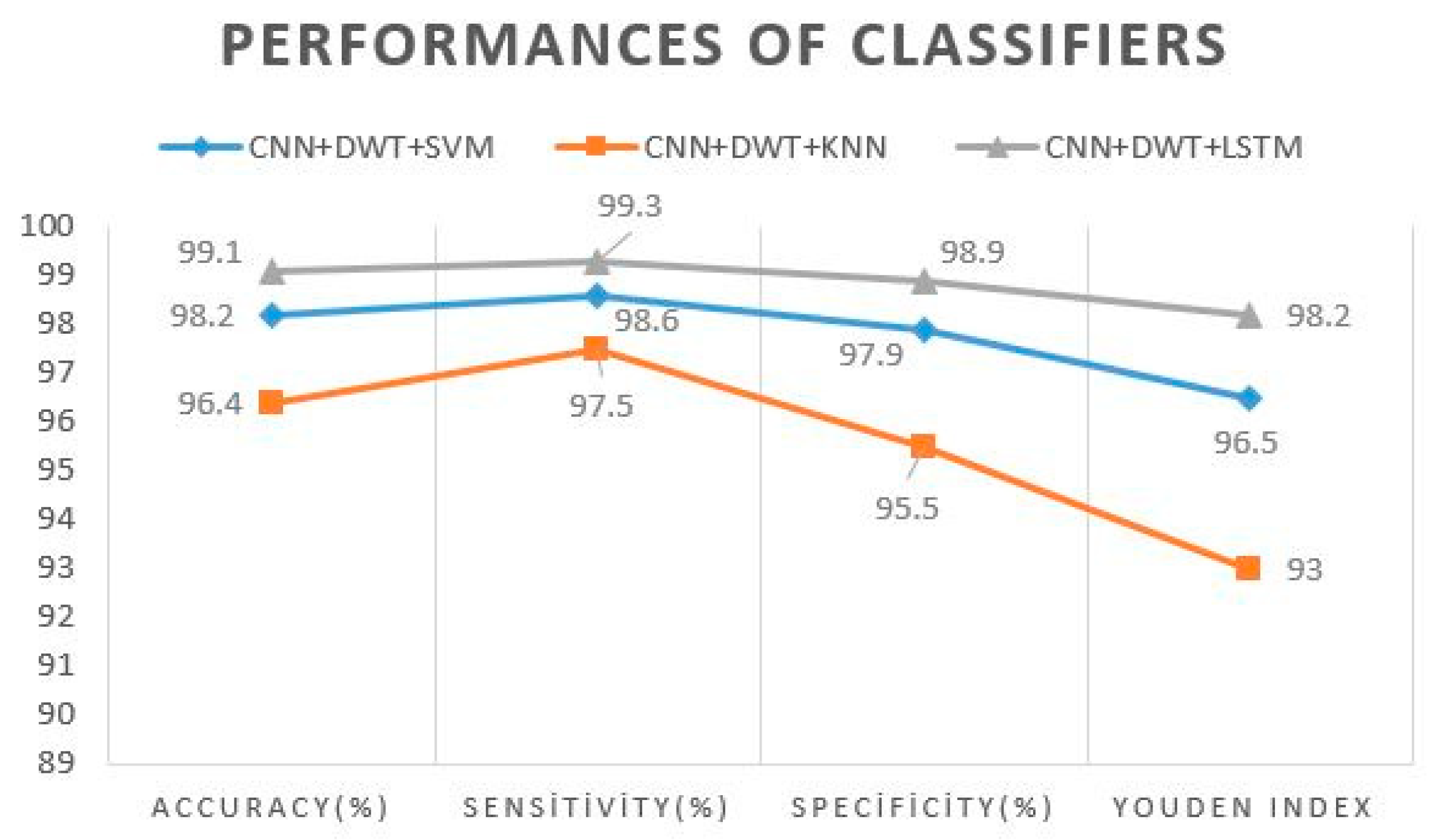
| CNN + DWT + SVM | 98.2 ± 1.4 | 98.6 ± 0.8 | 97.9 ± 2.3 | 0.96 ± 0.02 |
| CNN + DWT + KNN | 96.4 ± 0.6 | 97.5 ± 1.0 | 95.5 ± 0.9 | 0.93 ± 0.01 |
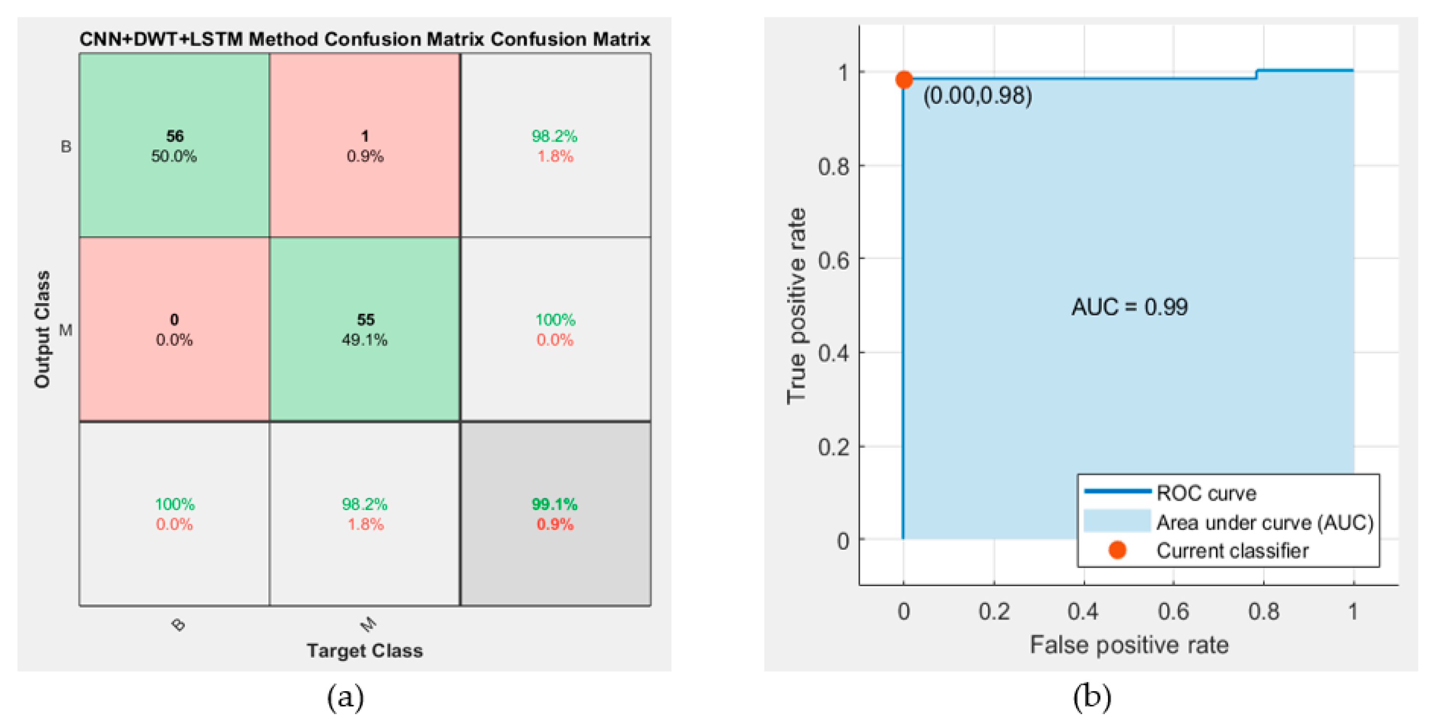
| CNN + DWT + LSTM | 99.1 ± 0.9 | 99.3 ± 1.0 | 98.9 ± 1.0 | 0.98 ± 0.01 |
| Method | Accuracy (%) | Sensitivity (%) | Specificity (%) | Youden’s Index |
|---|---|---|---|---|
| CNN + DCT + LSTM | 98.2 ± 1.1 | 98.2 ± 1.3 | 98.2 ± 1.3 | 0.96 ± 0.02 |
| CNN + FWHT + LSTM | 97.3 ± 0.6 | 97.2 ± 0.9 | 97.5 ± 1.0 | 0.94 ± 0.01 |
| CNN + DWT + LSTM | 99.1 ± 0.9 | 99.3 ± 1.0 | 98.9 ± 1.0 | 0.98 ± 0.01 |
| Image Size | Method | Accuracy (%) | Sensitivity (%) | Specificity (%) | Youden’s Index |
|---|---|---|---|---|---|
| Raw CT Images | CNN [30] Softmax | 94.6 | 92.8 | 96.4 | 0.89 |
| Raw CT Images | CNN + DWT + LSTM | 99.1 | 99.3 | 98.9 | 0.98 |
| Method | Accuracy (%) | Sensitivity (%) | Specificity (%) | Youden’s Index |
|---|---|---|---|---|
| CNN + KNN | 83.6 ± 0.01 | 83.6 ± 0.01 | 91.8 ± 0.005 | 0.75 ± 0.01 |
| CNN + SVM | 87.3 ± 0.01 | 87.3 ± 0.01 | 93.6 ± 0.008 | 0.81 ± 0.02 |
| CNN + LSTM | 87.5 ± 0.01 | 87.5 ± 0.01 | 93.7 ± 0.007 | 0.81 ± 0.02 |
| CNN + DWT + KNN | 85.91 ± 0.02 | 85.91 ± 0.02 | 92.95 ± 0.01 | 0.78 ± 0.03 |
| CNN + DWT + SVM | 92.09 ± 0.008 | 92.08 ± 0.008 | 96.04 ± 0.004 | 0.88 ± 0.01 |
| CNN + DWT + LSTM | 98.66 ± 0.01 | 98.66 ± 0.01 | 99.33 ± 0.008 | 0.98 ± 0.02 |
© 2019 by the authors. Licensee MDPI, Basel, Switzerland. This article is an open access article distributed under the terms and conditions of the Creative Commons Attribution (CC BY) license (http://creativecommons.org/licenses/by/4.0/).
Share and Cite
Kutlu, H.; Avcı, E. A Novel Method for Classifying Liver and Brain Tumors Using Convolutional Neural Networks, Discrete Wavelet Transform and Long Short-Term Memory Networks. Sensors 2019, 19, 1992. https://doi.org/10.3390/s19091992
Kutlu H, Avcı E. A Novel Method for Classifying Liver and Brain Tumors Using Convolutional Neural Networks, Discrete Wavelet Transform and Long Short-Term Memory Networks. Sensors. 2019; 19(9):1992. https://doi.org/10.3390/s19091992
Chicago/Turabian StyleKutlu, Hüseyin, and Engin Avcı. 2019. "A Novel Method for Classifying Liver and Brain Tumors Using Convolutional Neural Networks, Discrete Wavelet Transform and Long Short-Term Memory Networks" Sensors 19, no. 9: 1992. https://doi.org/10.3390/s19091992
APA StyleKutlu, H., & Avcı, E. (2019). A Novel Method for Classifying Liver and Brain Tumors Using Convolutional Neural Networks, Discrete Wavelet Transform and Long Short-Term Memory Networks. Sensors, 19(9), 1992. https://doi.org/10.3390/s19091992