X-Ray Pulsar-Based Navigation Considering Spacecraft Orbital Motion and Systematic Biases


Abstract
:1. Introduction
2. Signal Models of X-Ray Pulsars
2.1. Photon Arrival Rate Function at the SSB
- (1)
- The probability of detecting one photon in a time interval is when .
- (2)
- The probability of detecting more than one photon in is 0 when .
- (3)
- Nonoverlapping increments are independent.
2.2. Photon Arrival Rate Function at the Spacecraft
3. Dynamic and Measurement Models of Proposed Navigation Method
3.1. Dynamics Model
3.2. Measurement Models
3.2.1. PP and DF Measurements
3.2.2. DPP Measurement
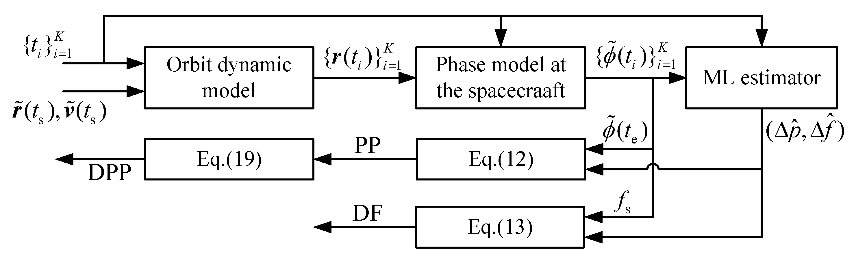
4. Measurements Estimation and Fusion Filtering
4.1. ML Estimator
4.2. Modified Unscented Kalman Filter
5. Photon-Level Simulations and Discussion
6. Conclusions
Author Contributions
Funding
Conflicts of Interest
Appendix A
| time varying photon arrival rate function at the SSB | |
| effective source arrival rate | |
| effective background arrival rate | |
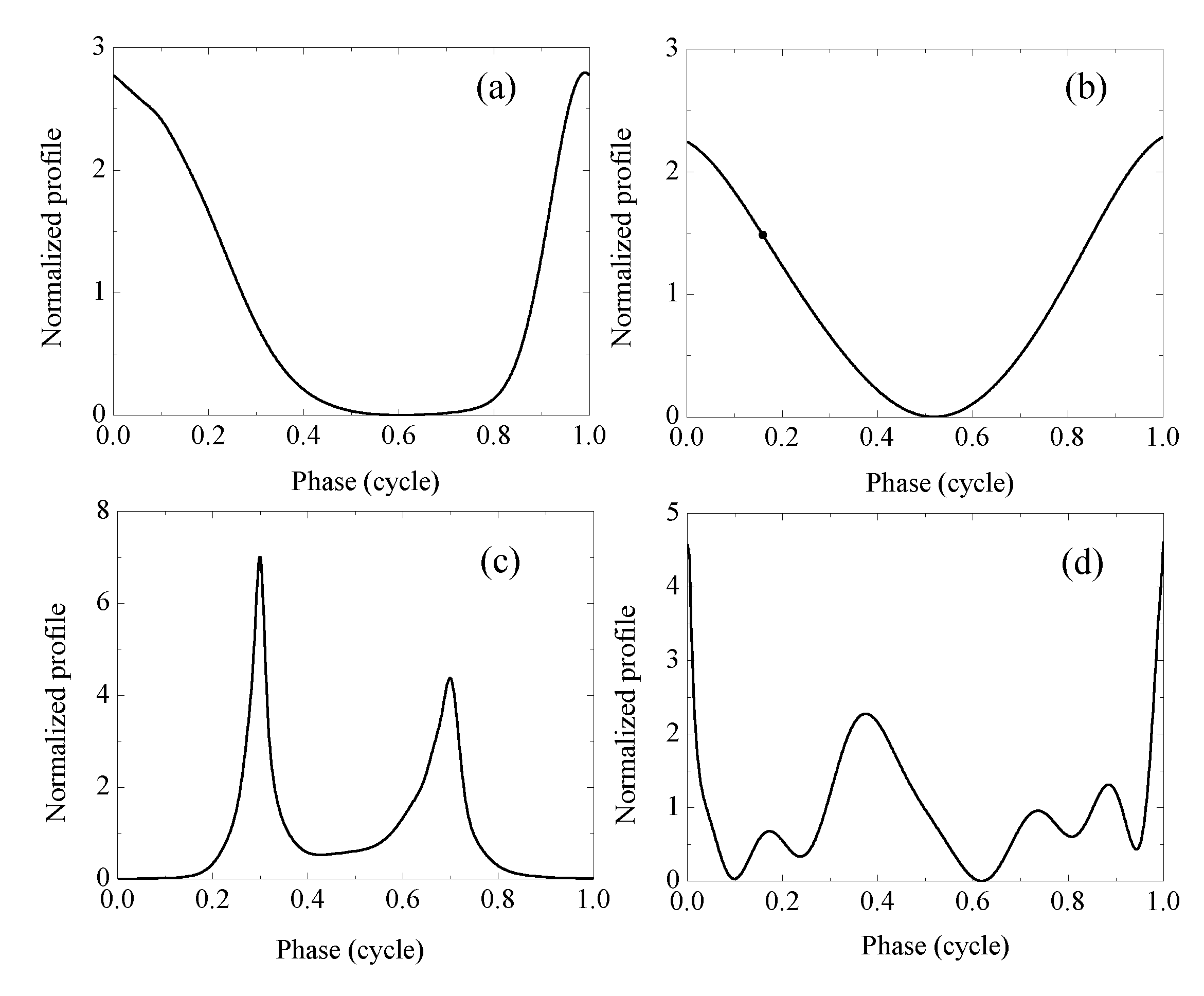
| normalized pulsar profile | |
| observed phase at the SSB with respect to the coordinate time seen at the SSB | |
| initial phase at a reference time seen at the SSB | |
| spacecraft’s coordinate in the SSB coordinate frame at the spacecraft proper time t | |
| spacecraft’s velocity in the SSB coordinate frame at the spacecraft proper time t | |
| n | directional vector from the SSB to the pulsar |
| photon arrival rate function at the spacecraft | |
| offset of proper time a photon arrives at the spacecraft compared to the arrival SSB-based coordinate time of the same photon at the SSB | |
| speed of light | |
| distance between the Sun and the pulsar | |
| position of SSB with respect to the Sun | |
| gravitational constant of Sun | |
| velocity vector of Earth with respect to the SSB | |
| total periodic correction items | |
| position of the spacecraft predicted by the orbit dynamics | |
| velocity of the spacecraft predicted by the orbit dynamics | |
| position error | |
| velocity error | |
| parallax delay corresponding to position | |
| Sun’s Shapiro delay corresponding to position | |
| Einstein delay corresponding to velocity | |
| pulsar phase model at the spacecraft derived by the spacecraft state with errors | |
| spacecraft’s position in the J2000.0 Earth Centered Inertial (ECI) coordinate system | |
| spacecraft’s velocity in the J2000.0 Earth Centered Inertial (ECI) coordinate system | |
| time interval of a filtering period | |
| estimated phase at the time as seen at the spacecraft | |
| estimated Doppler frequency at the time as seen at the spacecraft | |
| acceleration of spacecraft | |
| state vector of spacecraft with respect to the Earth | |
| process noise vector | |
| velocity noise vector | |
| acceleration noise vector | |
| pulse phase delay | |
| Doppler frequency offset | |
| Earth position vector relative to the SSB | |
| phase noise | |
| estimated pulse phase delay | |
| estimated Doppler frequency offset | |
| frequency noise | |
| measured pulsar direction vector | |
| pulsar direction error | |
| measured distance between the Sun and the pulsar | |
| pulsar distance error | |
| corresponding systematic biases caused by | |
| corresponding systematic biases caused by | |
| corresponding systematic biases caused by | |
| spacecraft’s maximum velocity in the SSB coordinate frame | |
| the difference of and the estimated phase of the previous filtering period, | |
| PP measurement vector of the navigation filter | |
| DF measurement vector of the navigation filter | |
| PP noise vector of the navigation filter | |
| DF noise vector of the navigation filter | |
| DPP measurement vector of the navigation filter | |
| DPP noise vector of the navigation filter |
References
- Lyne, A.; Hobbs, G.; Kramer, M.; Stairs, I.; Stappers, B. Switched Magnetospheric Regulation of Pulsar Spin-Down. Science 2010, 329, 408–412. [Google Scholar] [CrossRef]
- Emadzadeh, A.A. On modeling and pulse phase estimation of X-ray pulsars. IEEE Trans. Signal Process 2010, 58, 4484–4495. [Google Scholar] [CrossRef]
- Hobbs, G.; Lyne, A.; Kramer, M. An analysis of the timing irregularities for 366 pulsars. Mon. Not. R. Astron. Soc. 2010, 402, 1027–1048. [Google Scholar]
- Sun, H.F.; Bao, W.M.; Fang, H.Y.; Li, X.P. Effect of stability of X-ray pulsar profiles on range measurement accuracy in X-ray pulsar navigation. Acta Phys. Sin. 2014, 63, 069701. [Google Scholar]
- Golshan, A.R.; Sheikh, S.I. On pulse phase estimation and tracking of variable celestial X-ray sources. In Proceedings of the ION 63rd Annual Meeting, Cambridge, MA, USA, 23–25 April 2007; pp. 410–412. [Google Scholar]
- Emadzadeh, A.A.; Speyer, J.L. X-ray pulsar-based relative navigation using epoch folding. IEEE Trans. Aerosp. Electron. Syst. 2011, 47, 2317–2328. [Google Scholar] [CrossRef]
- Huang, L.W.; Liang, B.; Zhang, T.; Zhang, C. Navigation using binary pulsars. Sci. China-Phys. Mech. Astron. 2012, 55, 527–539. [Google Scholar] [CrossRef]
- Coles, W.; Hobbls, G.; Champion, D.J.; Manchester, R.N.; Verbiest, J.P.W. Pulsar timing analysis in the presence of correlated noise. Mon. Not. R. Astron. Soc. 2011, 418, 561–570. [Google Scholar] [CrossRef]
- Ning, X.L.; Gui, M.; Fang, J.; Liu, G. Differential X-ray pulsar aided celestial navigation for Mars exploration. Aerosp. Sci. Technol. 2017, 62, 36–45. [Google Scholar] [CrossRef]
- Wang, Y.D.; Zheng, W.; An, X.; Sun, S.; Li, L. XNAV/CNS Integrated Navigation Based on Improved Kinematic and Static Filter. J. Navig. 2013, 66, 899–918. [Google Scholar] [CrossRef]
- van Haasteren, R.; Levin, Y. Understanding and analyzing time-correlated stochastic signals in pulsar timing. Mon. Not. R. Astron. Soc. 2013, 428, 1147–1159. [Google Scholar] [CrossRef]
- Ashby, N.; Golshan, A.R. Minimum uncertainties in position and velocity determination using X-ray photons from millisecond pulsars. In Proceedings of the ION NTM, San Diego, CA, USA, 28–30 January 2008; pp. 110–118. [Google Scholar]
- Song, S.; Xu, L.P.; Zhang, H.; Bai, Y. Novel X-ray Communication Based XNAV Augmentation Method Using X-ray Detectors. Sensors 2015, 15, 22325–22342. [Google Scholar] [CrossRef]
- Rinauro, S.; Colonnese, S.; Scarano, G. Fast near-maximum likelihood phase estimation of X-ray pulsars. Signal Process. 2013, 93, 326–331. [Google Scholar] [CrossRef]
- Emadzadeh, A.A.; Speyer, J.L. Navigation in Space by X-ray Pulsars; Springer: Berlin, Germany, 2011. [Google Scholar]
- Wang, Y.; Zheng, W.; Sun, S.; Li, L. X-ray pulsar-based navigation using time-differenced measurement. Aerosp. Sci. Technol. 2014, 36, 27–35. [Google Scholar] [CrossRef]
- Anderson, K.D.; Pines, D.J. Methods of pulse phase tracking for X-ray pulsar based spacecraft navigation using low flux pulsars. In Proceedings of the SpaceOps 2014 Conference, Pasadena, CA, USA, 26–27 September 2014; p. 1858. [Google Scholar]
- Anderson, K.D.; Pines, D.J. Experimental Validation of Pulse Phase Tracking for X-ray Pulsar Based Spacecraft Navigation. In Proceedings of the AIAA Guidance, Navigation, and Control (GNC) Conference, Boston, MA, USA; 2013; p. 5202. [Google Scholar]
- Sun, H.F.; Bao, W.M.; Xue, M.F.; Fang, H.Y. A Doppler shift estimation method in X-Ray pulsar based navigation. J. Astron. 2015, 36, 364–373. [Google Scholar]
- Winternitz, L.M.B.; Hassouneh, M.A.; Mitchell, J.W.; Valdez, J.E.; Price, S.R.; Semper, S.R.; Yu, W.H.; Ray, P.S.; Wood, K.S.; Arzoumanian, Z.; et al. X-ray pulsar navigation algorithms and testbed for SEXTANT. In Proceedings of the Aerospace Conference IEEE, Big Sky, MT, USA, 7–14 March 2015. [Google Scholar]
- Liu, J.; Fang, J.C.; Kang, Z.W.; Wu, J.; Ning, X.L. Novel algorithm for X-ray pulsar navigation against Doppler effects. IEEE Trans. Aerosp. Electron. Syst. 2015, 51, 228–241. [Google Scholar] [CrossRef]
- Wang, Y.D.; Zheng, W. Pulsar phase and Doppler frequency estimation for XNAV using on-orbit epoch folding. IEEE Trans. Aerosp. Electron. Syst. 2016, 52, 2210–2219. [Google Scholar] [CrossRef]
- Xiong, K.; Wei, C.L.; Liu, L.D. The use of X-ray pulsars for aiding navigation of satellites in constellations. Acta Astron. 2009, 64, 427–436. [Google Scholar]
- Liu, J.; Ma, J.; Tian, J.W.; Kang, Z.W. X-ray pulsar navigation method for spacecraft with pulsar direction error. Adv. Space Res. 2010, 46, 1409–1417. [Google Scholar] [CrossRef]
- Miguez, J. Analysis of selection methods for cost-reference particle filtering with applications to maneuvering target tracking and dynamic optimization. Dig. Signal Process. 2007, 17, 787–807. [Google Scholar] [CrossRef]
- Crisan, D.; Miguez, J. Nested particle filters for online parameter estimation in discrete-time state-space Markov models. Statistics 2015, 24, 3039–3086. [Google Scholar] [CrossRef]
- Martino, L.; Read, J.; Elvira, V.; Louzada, F. Cooperative parallel particle filters for online model selection and applications to urban mobility. Dig. Signal Process. 2017, 60, 172–185. [Google Scholar] [CrossRef]
- Martino, L.; Elvira, V.; Camps-Valls, G. Distributed Particle Metropolis-Hastings schemes. In Proceedings of the IEEE Statistical Signal Processing Workshop (SSP), Freiburg, Germany, 10–13 June 2018. [Google Scholar]
- Sheikh, S.I. The Use of Variable Celestial X-ray Sources for Spacecraft Navigation. Doctoral’s Dissertation, Maryland University, College Park, MD, USA, 2005. [Google Scholar]
- Fu, L.Z.; Shuai, P.; Xue, M.F.; Sun, H.; Fang, H. The Research of X-Ray Pulsar Signals Simulation Method. In Proceedings of the 6th China Satellite Navigation Conference (CSNC), Xian, China, 13–15 May 2015. [Google Scholar]
- RXTE Cook Book. Available online: ftp://legacy.gsfc.nasa.gov/xte/doc/cook_book/ (accessed on 05 May 2015).
- Tian, F. Error estimation of pulsar timing based spacecraft autonomous positioning. Prog. Astron. 2011, 29, 97–104. [Google Scholar]
- Xue, M.F.; Li, X.P.; Sun, H.; Liu, B.; Fang, H.; Shen, L.-R. A new simulation method of X-ray pulsar signals. Acta Phys. Sin. 2015, 64, 219701. [Google Scholar]


| Name | Declination (°) | Right Ascension (°) | (kpc) | (1/s) | (1/s2) | Declination | Right Ascension | |
|---|---|---|---|---|---|---|---|---|
| B0833-45 | −2.79 | 263.55 | 3.9 | 1.59 × 10⁻³ | 11.197 | −1.56 × 10⁻¹¹ | −44 | 128 |
| B0540-69 | −68.6684 | 85.0465 | 47.3 | 5.15 × 10⁻³ | 19.802 | 0.000 × 10+0 | 200 | 40 |
| B1509-58 | −58.8642 | 228.4818 | 4.3 | 1.62 × 10⁻² | 6.629 | −6.74 × 10⁻¹¹ | 1000 | 90 |
| B0531+21 | 22.0145 | 83.6332 | 2 | 1.12 × 10⁻¹ | 29.982 | −3.79 × 10⁻¹⁰ | 60 | 5 |
| Orbit State | Value |
|---|---|
| x-axis position | −7385277.8 m |
| y-axis position | 34560765.34 m |
| z-axis position | −22339513.83 m |
| x-axis velocity | −1316.58 m/s |
| y-axis velocity | −1702.40 m/s |
| z-axis velocity | −2223.82 m/s |
| Measurement | Concept |
|---|---|
| PP | PP Pulse phase |
| DF | DF Doppler frequency |
| DPP | difference of and |
| PP | PP + DF | PP + DF + DPP | ||
|---|---|---|---|---|
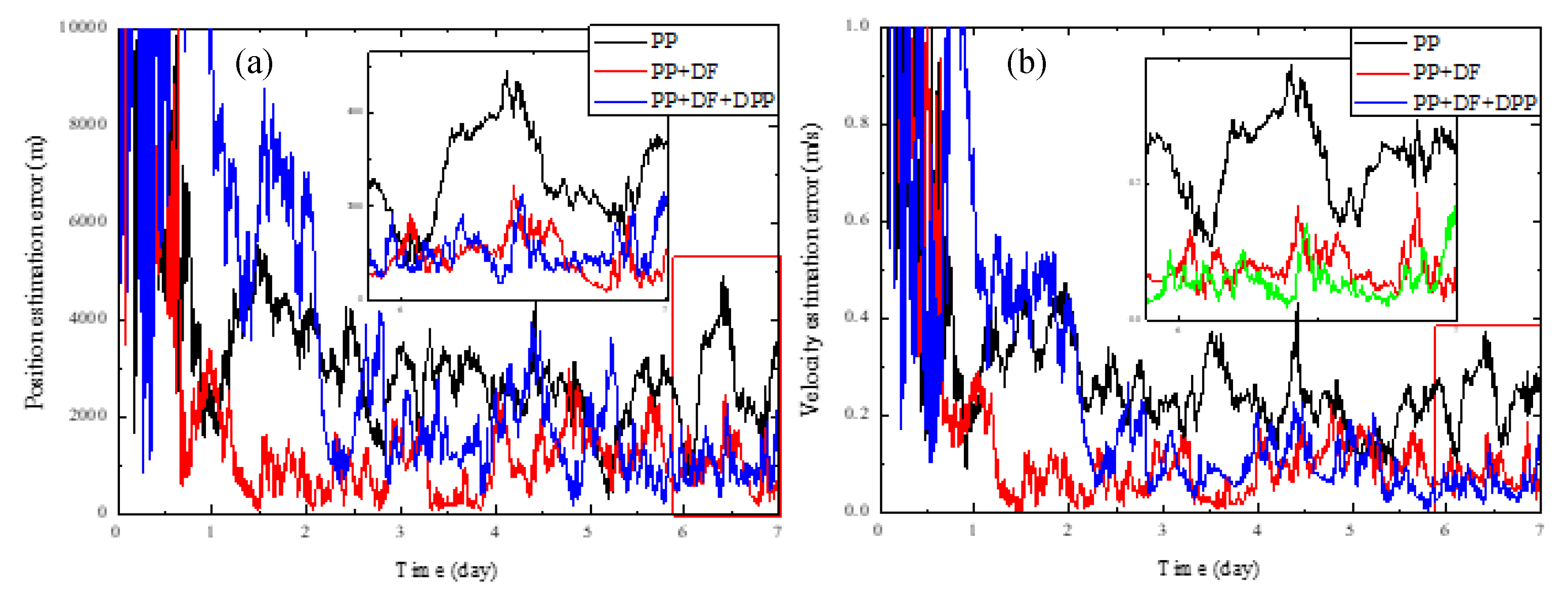
| Results without systematic errors | Position error (m) | 4906 | 3010 | 3297 |
| Velocity error (m/s) | 0.4355 | 0.2191 | 0.2214 | |
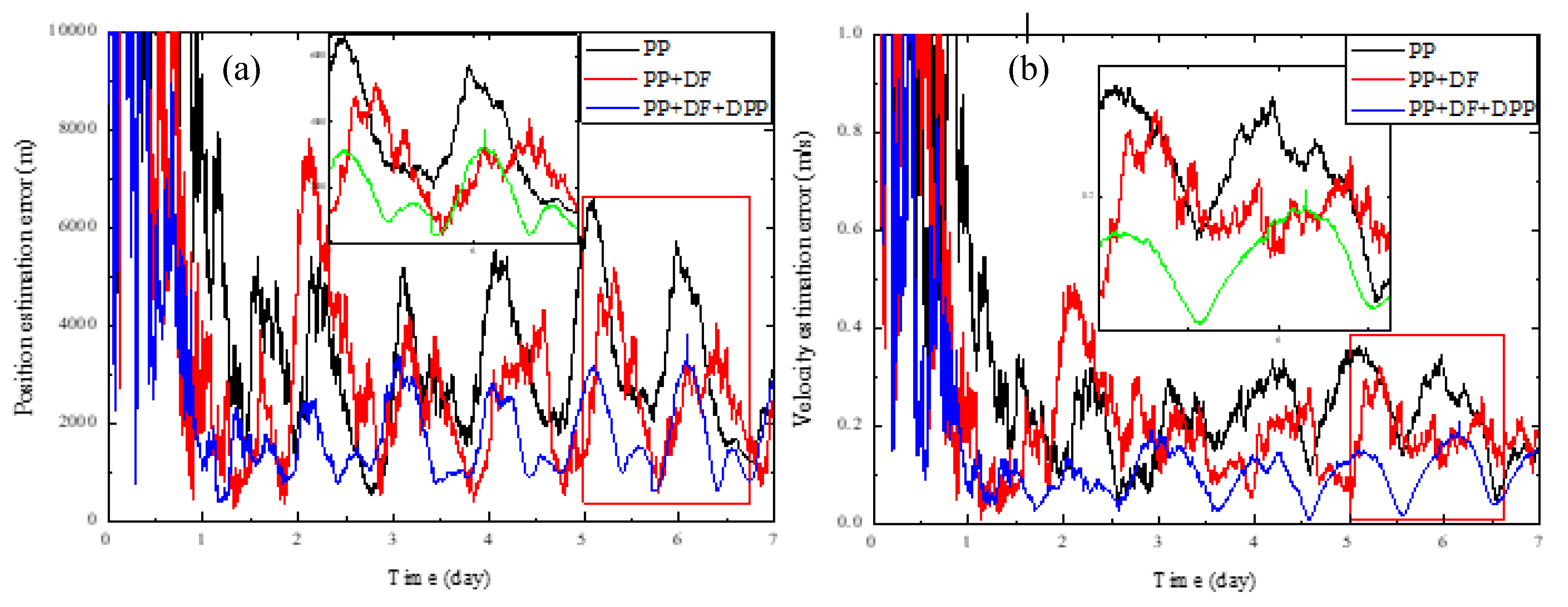
| Results with systematic errors | Position error (m) | 6591 | 5180 | 3820 |
| Velocity error (m/s) | 0.36 | 0.32 | 0.2301 |
| Initial Velocity Error | Position Error (m) (PP + DPP) | Position Error (m) (PP + DF + DPP) |
|---|---|---|
| [60 m/s, 60 m/s, 120 m/s] | 4084 | 3565 |
| [80 m/s, 80 m/s, 160 m/s] | 4367 | 3687 |
| [100 m/s, 100 m/s, 200 m/s] | 5298 | 3824 |
| [120 m/s,120 m/s, 240 m/s] | 6496 | 4078 |
| [140 m/s, 140 m/s, 280 m/s] | 7930 | 4307 |
| [160 m/s, 160 m/s, 320 m/s] | 9477 | 4472 |
© 2019 by the authors. Licensee MDPI, Basel, Switzerland. This article is an open access article distributed under the terms and conditions of the Creative Commons Attribution (CC BY) license (http://creativecommons.org/licenses/by/4.0/).
Share and Cite
Xue, M.; Shi, Y.; Guo, Y.; Huang, N.; Peng, D.; Luo, J.; Shentu, H.; Chen, Z. X-Ray Pulsar-Based Navigation Considering Spacecraft Orbital Motion and Systematic Biases. Sensors 2019, 19, 1877. https://doi.org/10.3390/s19081877
Xue M, Shi Y, Guo Y, Huang N, Peng D, Luo J, Shentu H, Chen Z. X-Ray Pulsar-Based Navigation Considering Spacecraft Orbital Motion and Systematic Biases. Sensors. 2019; 19(8):1877. https://doi.org/10.3390/s19081877
Chicago/Turabian StyleXue, Mengfan, Yifang Shi, Yunfei Guo, Na Huang, Dongliang Peng, Ji’an Luo, Han Shentu, and Zhikun Chen. 2019. "X-Ray Pulsar-Based Navigation Considering Spacecraft Orbital Motion and Systematic Biases" Sensors 19, no. 8: 1877. https://doi.org/10.3390/s19081877
APA StyleXue, M., Shi, Y., Guo, Y., Huang, N., Peng, D., Luo, J., Shentu, H., & Chen, Z. (2019). X-Ray Pulsar-Based Navigation Considering Spacecraft Orbital Motion and Systematic Biases. Sensors, 19(8), 1877. https://doi.org/10.3390/s19081877