Fault Detection in Wireless Sensor Networks through the Random Forest Classifier


 , and
, and
Abstract
1. Introduction
- software failures,
- hardware failures, and
- communication failures.
- Offset fault: Due to a calibration error in a sensing unit, a displacement value is added to the actual sensed data.
- Gain fault: When the change rate of sensed data is different from the expected rate.
- Stuck-at fault: When the variation in sensed data series is zero.
- Out of bounds: When the observed values are out of bounds of expected series.
- Spike fault: When the rate of change of measured time series with the predicted time series is more than the expected changing trend.
- Noise fault: When a randomly-distributed number is added to the expected value.
- Data loss fault: When there are some missing data during a specific time interval in the sensed values.
- Random fault: This is an instant error, where data are perturbed for an observation.
- Supervised learning: Data mining techniques are applied to data with a predetermined label of the classes.
- Unsupervised learning: The techniques are applied to non-labeled data. Data are classified with no previous knowledge.
- Semi-supervised learning: This is a hybrid of supervised and unsupervised learning.
1.1. Motivation
1.2. Challenges and Problem Statement
- There are very limited means and resources at the node level, which compel nodes to use classifiers [1] because they do not require complex computation.
- The sensor nodes are stationed in dangerous and risky environments, e.g., indoors, war zones, tropical storms, earthquakes, etc.
- The fault detection process [5] should be precise and rapid to avoid any loss, e.g., the process should recognize the difference between abnormal and normal cases, so that it can contain loss in the case of acquiring erroneous data that could lead to misleading results.
1.3. Contributions
- In this paper, two more faults are induced in the datasets, which are listed below:
- -
- spike fault, and
- -
- data loss fault.
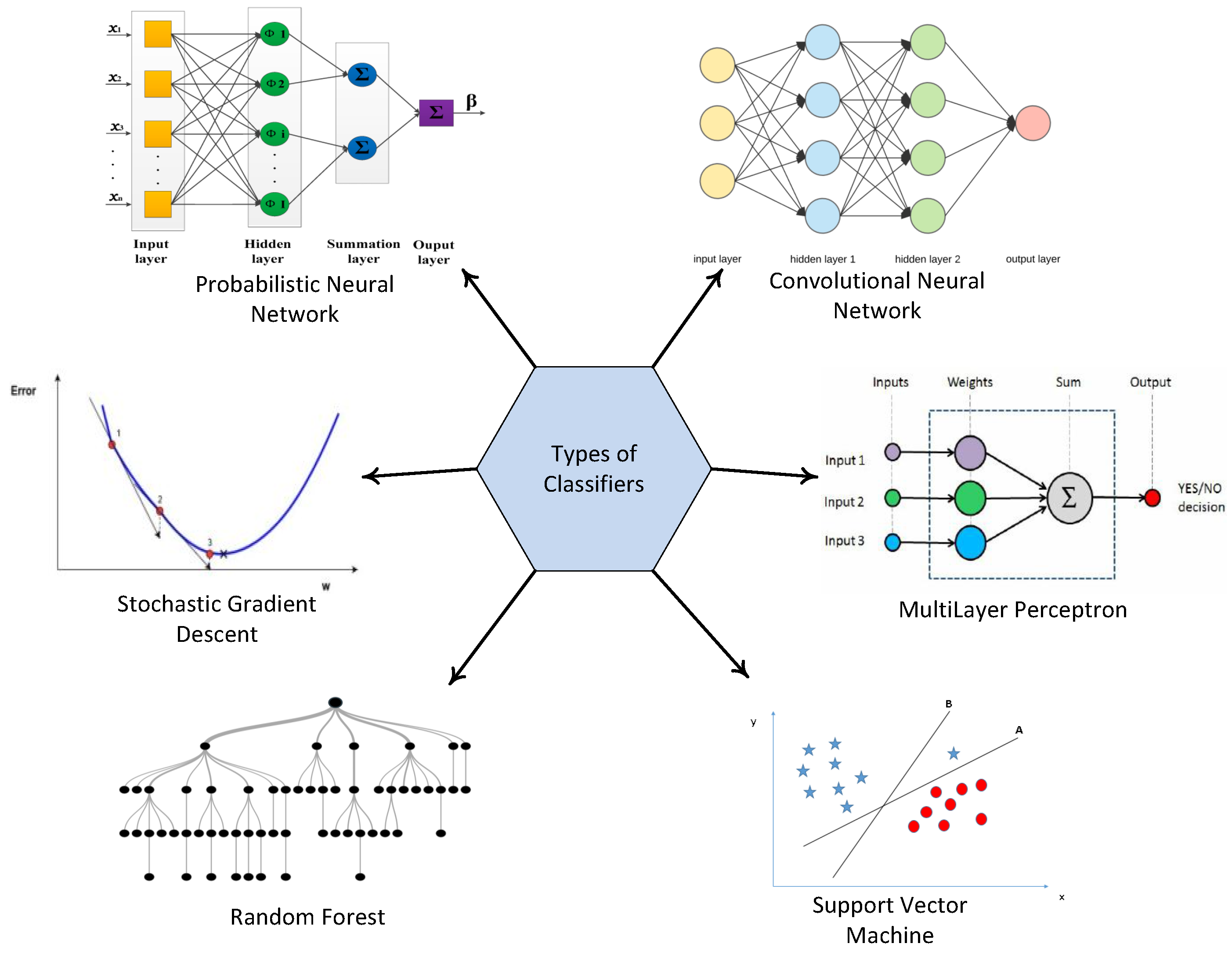
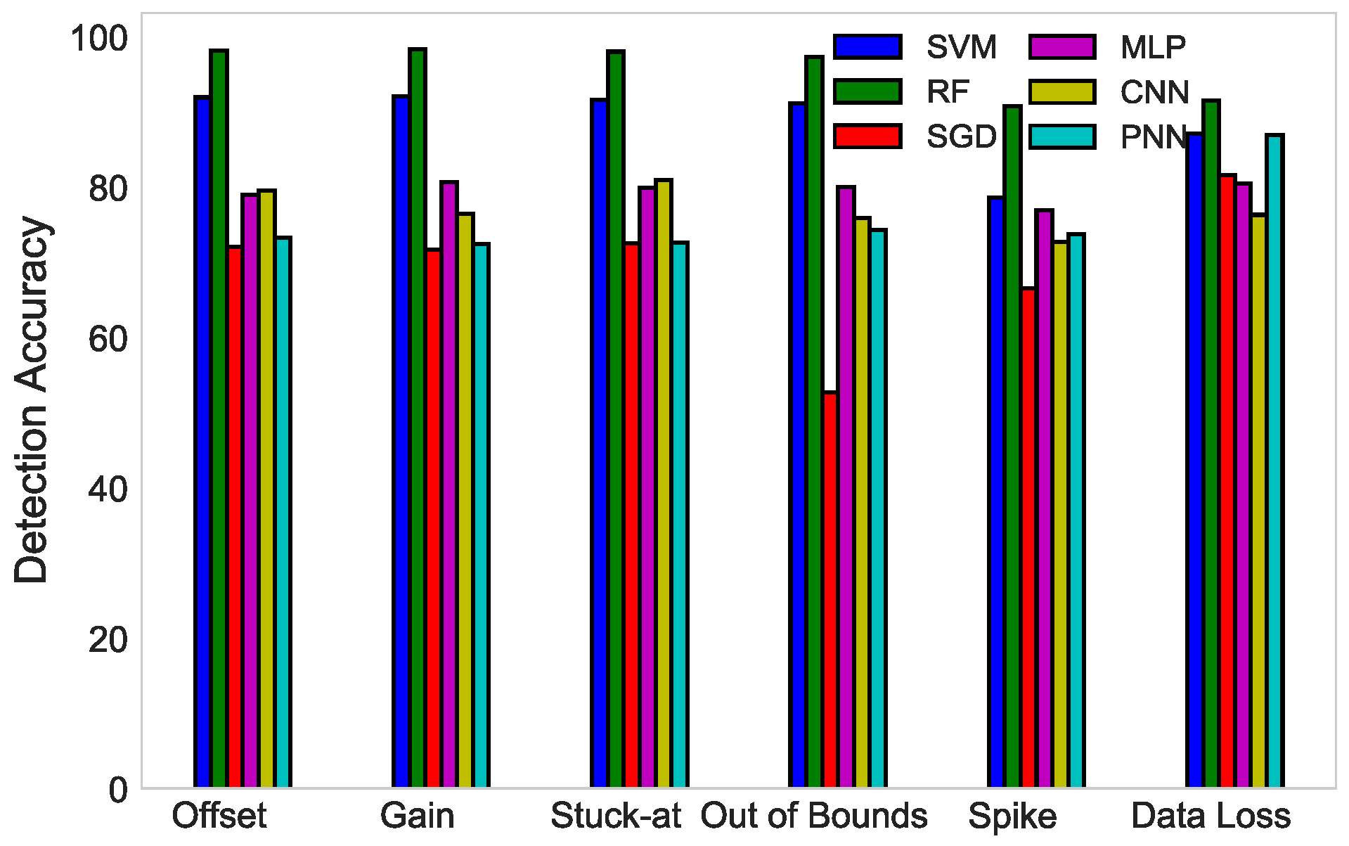
- Following that, six classifiers are applied on the datasets, and an extensive simulation study is conducted in our scenario to detect faults in WSN. The classifiers used are: SVM, RF, SGD, MLP, CNN, and PNN.
- The performance of classifiers is evaluated by four widely-used measures, which are stated below:
- -
- Detection Accuracy (DA),
- -
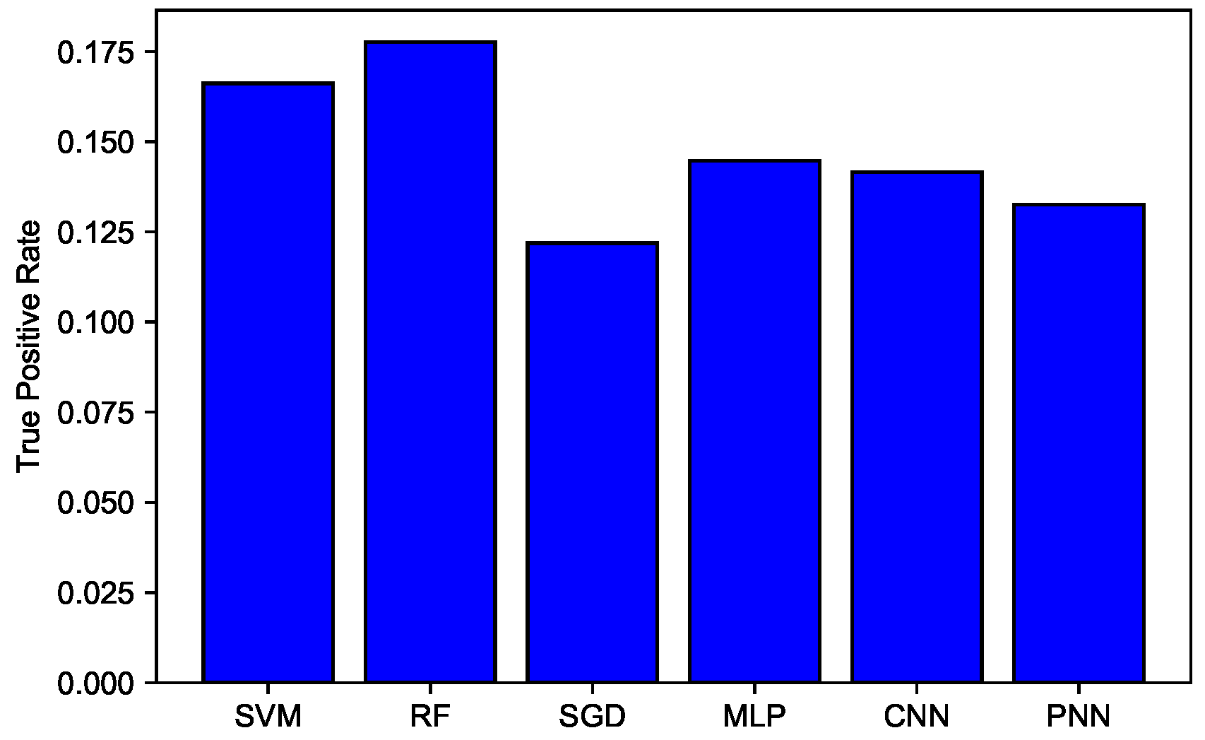
- True Positive Rate (TPR),
- -
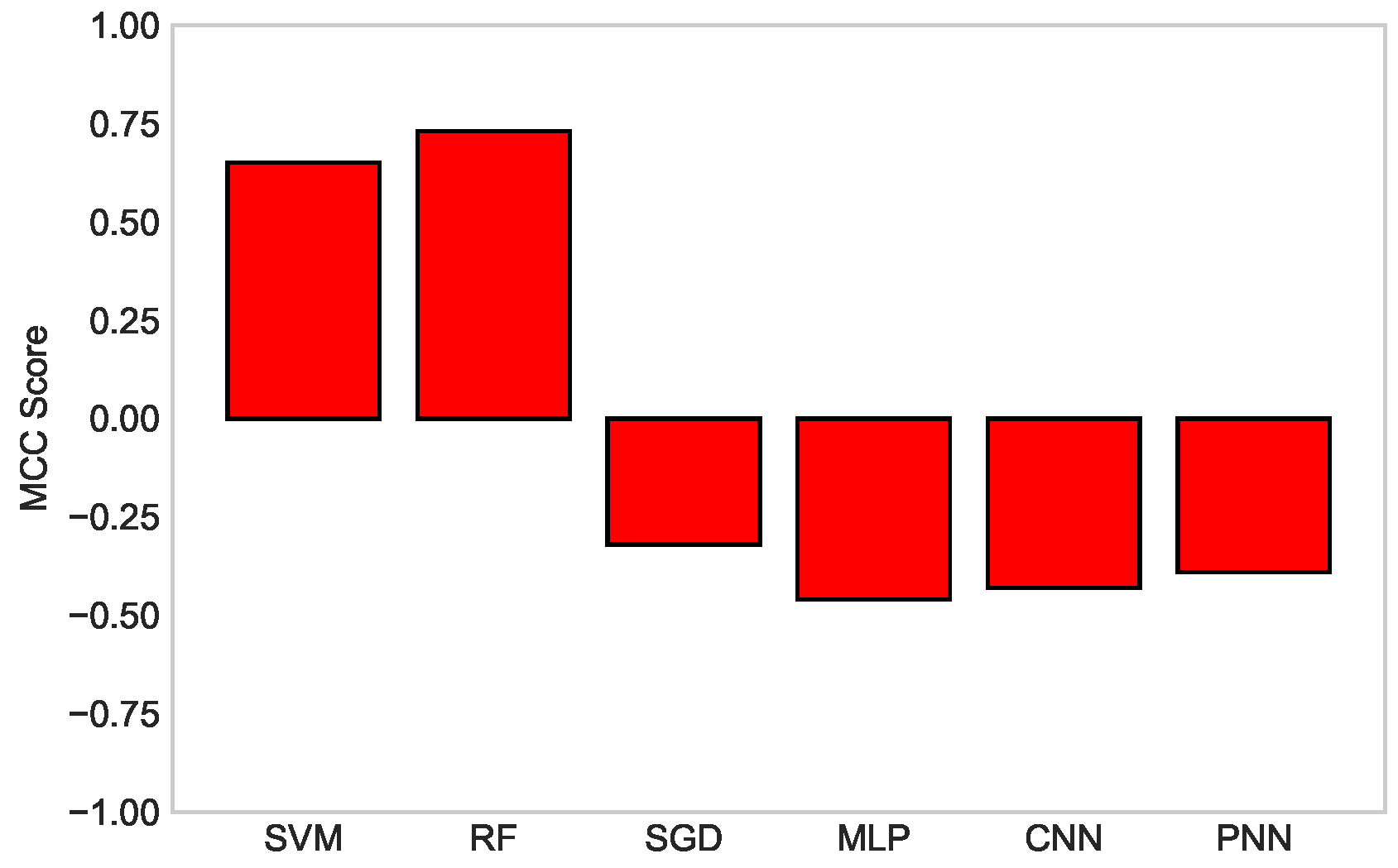
- Matthews Correlation Coefficient (MCC), and
- -
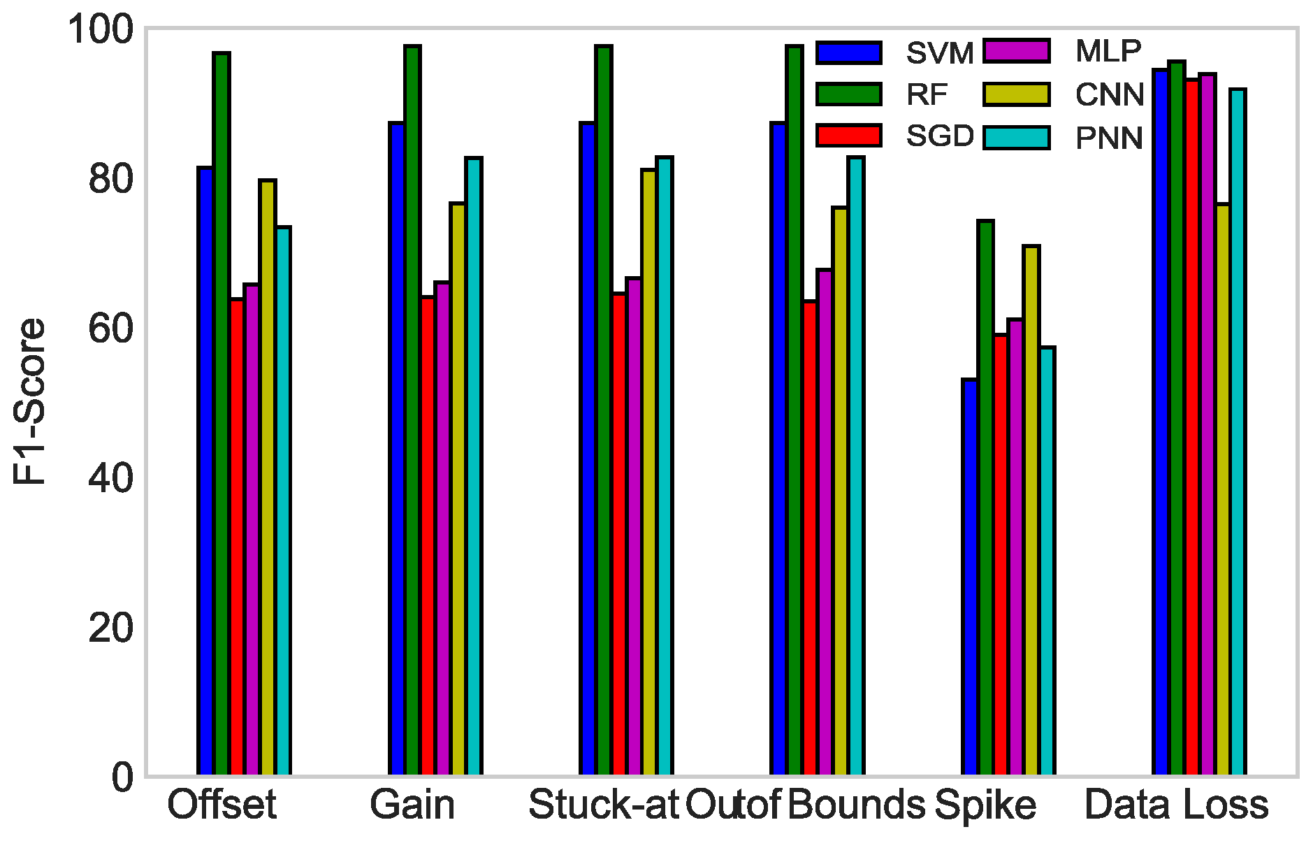
- F1-score.
2. Related Work
3. Faults in WSNs
3.1. Gain Fault
3.2. Offset Fault
3.3. Stuck-at Fault
3.4. Spike Fault
3.5. Data Loss Fault
3.6. Out of Bounds
4. Classifiers
4.1. SVM
4.2. MLP
4.3. CNN
- In the convolutional step, there are three important parts to mention: the input, the feature detector, and the feature map. The main objective of this step is to reduce the size of the input, which would eventually make the process faster and easier.
- The rectified linear unit is the rectifier function (activation function) that increases the non-linearity in CNN.
- Pooling enables CNN to detect features in various images, irrespective of the difference in lighting or their variant angles.
- Once the pooled feature map is obtained, the next step is to flatten it. Flattening means converting the entire pooled feature map image into a single column, which is then fed to the neural network for further processing.
- The last layer is made up of an input layer, a fully-connected layer, and an output layer. The output layer generates the predicted class. The information is passed through the network, and the error of prediction is calculated. The error is then transmitted back to the network for improvement in prediction.
4.4. RF
- The first step is to create an RF tree. It is further elaborated in the following five stages:
- -
- K number of random features are selected from total features m, where K is less than m,
- -
- within the selected features, node d is determined using the best split point,
- -
- those nodes are further distributed into daughter nodes through best split,
- -
- the first three steps are repeated until l number of nodes are obtained,
- -
- all of the above steps are repeated for n times to achieve p number of trees, where n is not equal to p.
- The next step is to classify the data based on an RF tree that has been created in the first step. It has the following stages:
- -
- with the rules created for each randomly-formulated decision tree and test features, data are classified,
- -
- the votes are calculated for each target value,
- -
- the highest voted prediction target is considered to be the final result of the RF algorithm.
4.5. SGD
4.6. PNN
- Input layer: The first layer is the initiating layer of PNN. It has multiple neurons where each neuron represents a predictor variable. There are N number of groups, and neurons are used as categorical variables. Then, the range is standardized by dividing the subtracted median by the interquartile range. These values are used as an input for the next layer of neurons, which is a pattern layer.
- Pattern layer: This is the second layer of PNN. Each case contains a single neuron in the training dataset. The target value and predictor variables are stored together in a case. Then, a private neuron calculates the Euclidean Distance (ED) from the center point of all neurons. This process is repeated for each and every case. After that, ED is used with the radial basis kernel function along with the sigma values.
- Summation layer: The output of the pattern layer is a pattern neuron that is used as an input for the summation layer. In PNN, each category of target variables has one pattern neuron. After that, every hidden neuron stores the actual target category of each training case; these weighted values are streamed in the pattern neurons that are in compliance with the hidden neuron’s category. These values are added in pattern neurons for the determined class.
- Output layer: The weighted votes are compared in the output layer. The selection criteria for determining which vote should be used for predicting the target category are based on the comparison of weighted votes for each target class that is calculated in the second layer.
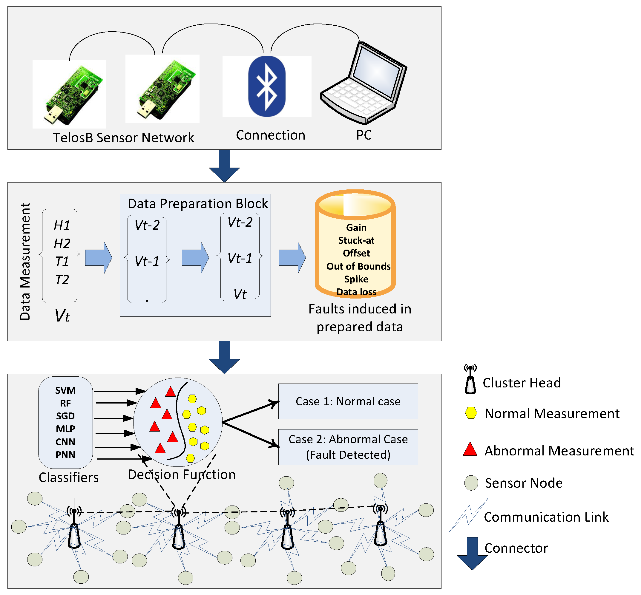
5. System Model
5.1. Phase 1
5.2. Phase 2
5.3. Phase 3
6. Simulations and Results
6.1. Datasets
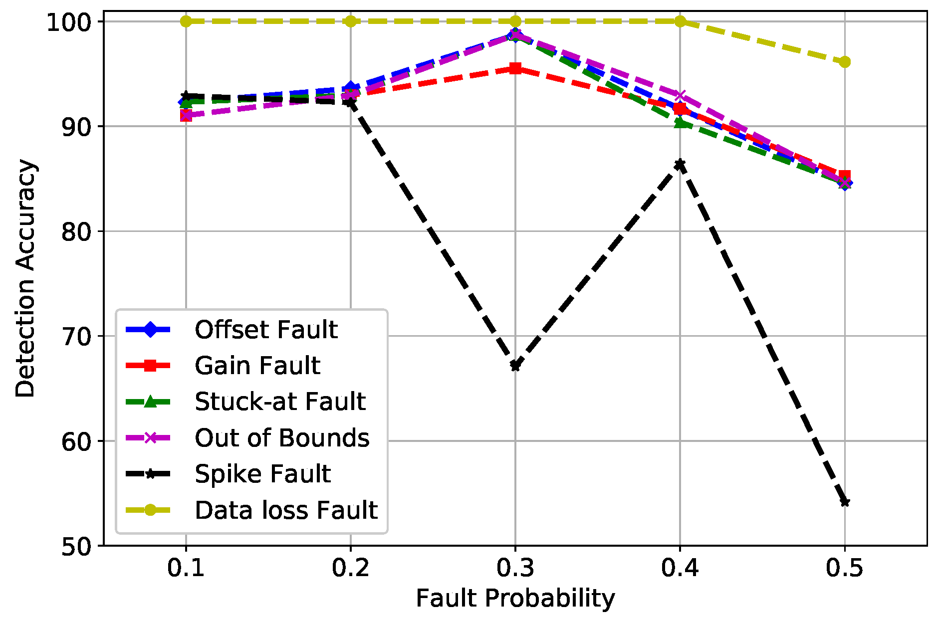
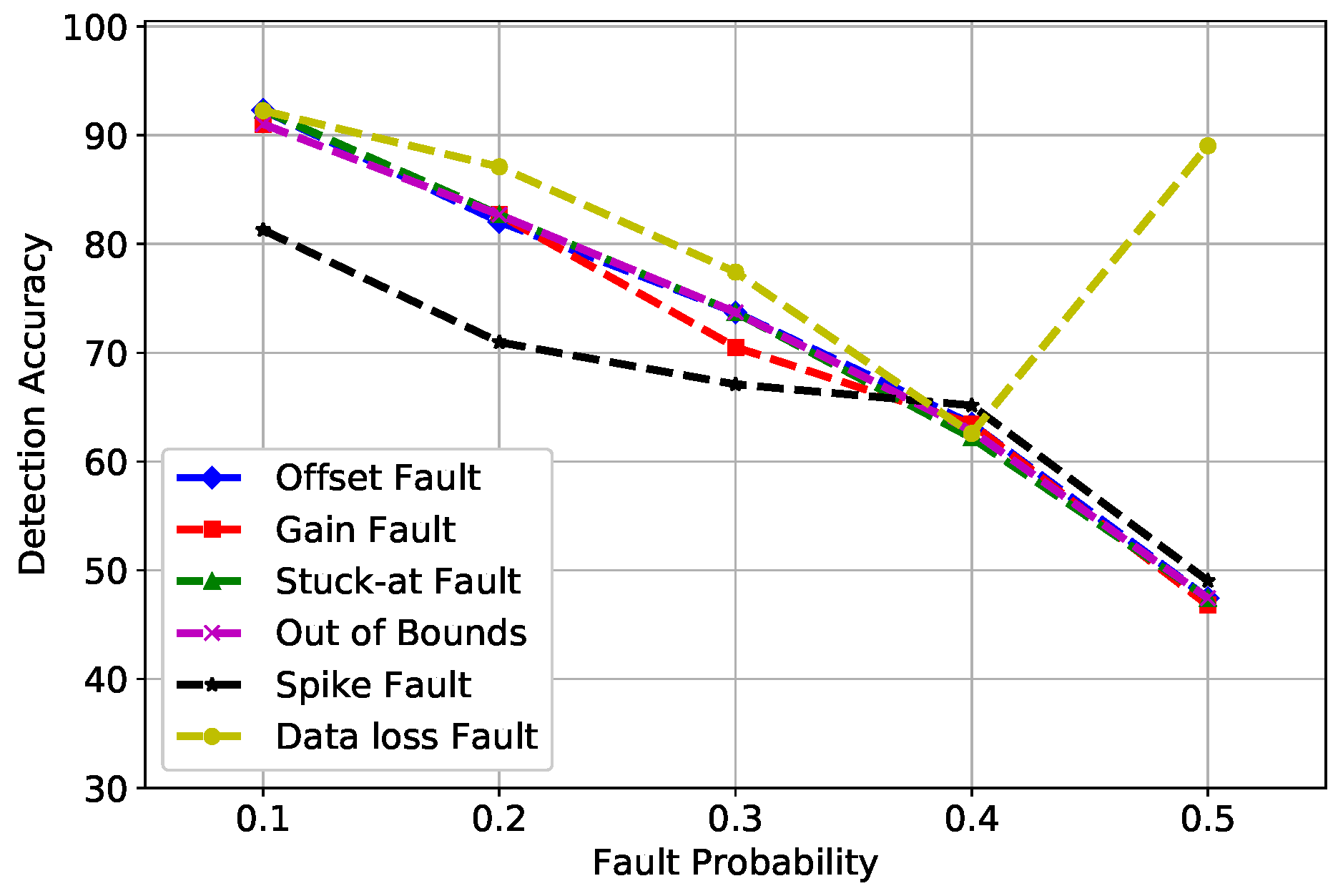
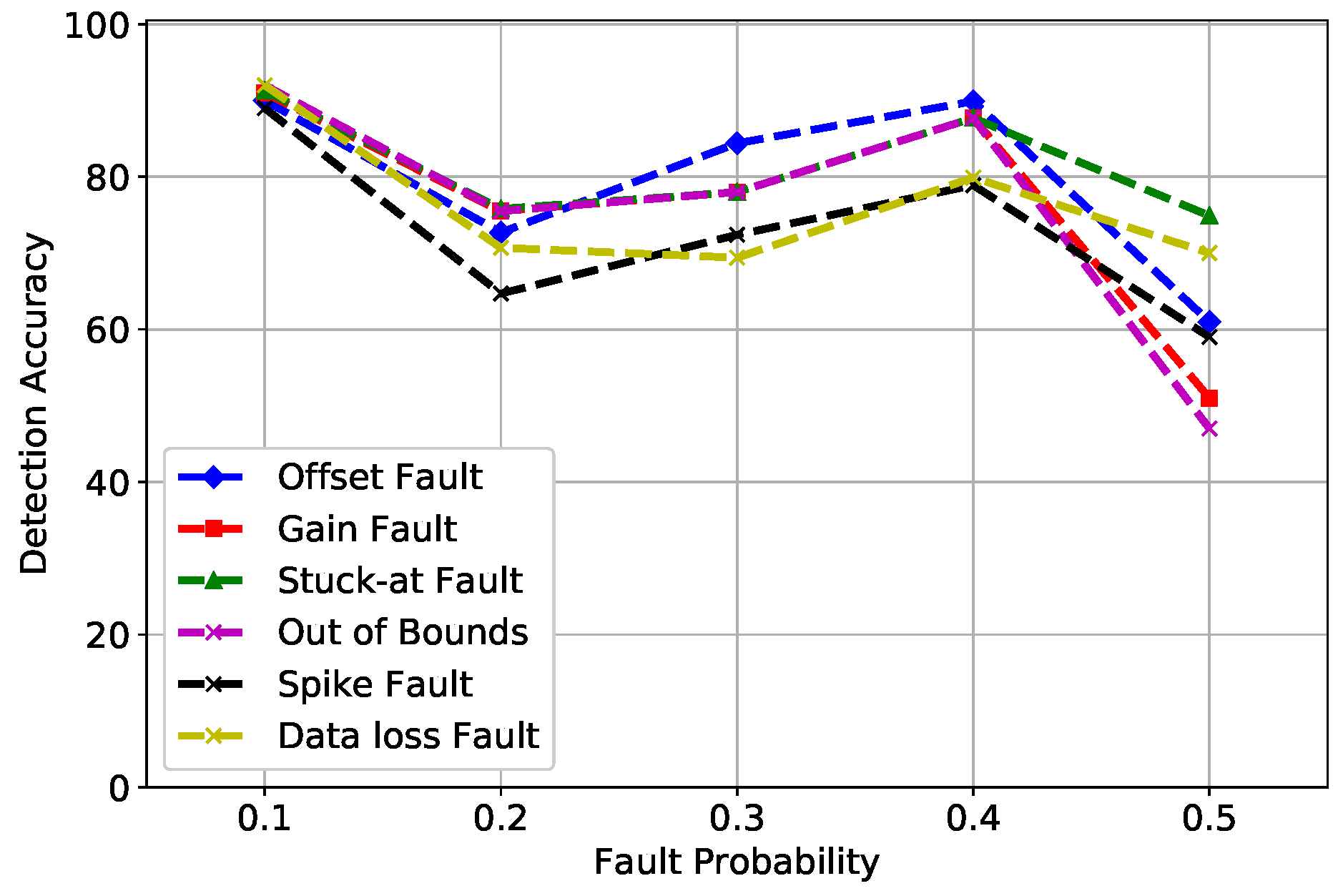
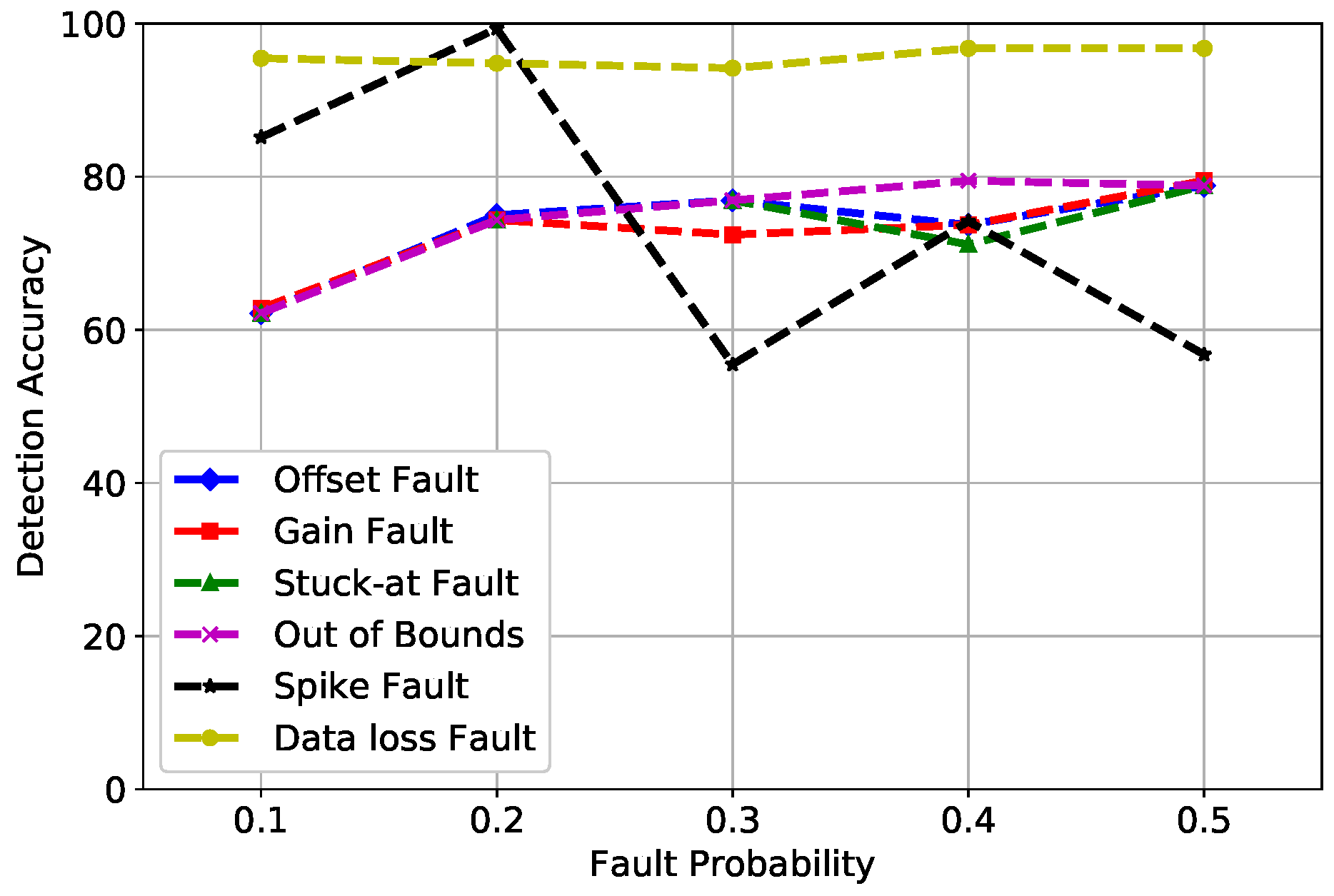
6.2. Results
7. Conclusions and Future Work
Author Contributions
Funding
Conflicts of Interest
References
- Zidi, S.; Moulahi, T.; Alaya, B. Fault detection in wireless sensor networks through SVM classifier. IEEE Sens. J. 2017, 18, 340–347. [Google Scholar] [CrossRef]
- Muhammed, T.; Shaikh, R.A. An analysis of fault detection strategies in wireless sensor networks. J. Netw. Comput. Appl. 2017, 78, 267–287. [Google Scholar] [CrossRef]
- Miao, X.; Liu, Y.; Zhao, H.; Li, C. Distributed Online One-Class Support Vector Machine for Anomaly Detection Over Networks. IEEE Trans. Cybern. 2018, 99, 1–14. [Google Scholar] [CrossRef]
- Gharghan, S.K.; Nordin, R.; Ismail, M.; Ali, J.A. Accurate wireless sensor localization technique based on hybrid PSO-ANN algorithm for indoor and outdoor track cycling. IEEE Sens. J. 2016, 16, 529–541. [Google Scholar] [CrossRef]
- Swain, R.R.; Khilar, P.M.; Dash, T. Neural network based automated detection of link failures in wireless sensor networks and extension to a study on the detection of disjoint nodes. J. Ambient Intell. Hum. Comput. 2018, 10, 593–610. [Google Scholar] [CrossRef]
- Cheng, Y.; Liu, Q.; Wang, J.; Wan, S.; Umer, T. Distributed Fault Detection for Wireless Sensor Networks Based on Support Vector Regression. Wirel. Commun. Mob. Comput. 2018. [Google Scholar] [CrossRef]
- Yuan, Y.; Li, S.; Zhang, X.; Sun, J. A Comparative Analysis of SVM, Naive Bayes and GBDT for Data Faults Detection in WSNs. In Proceedings of the 2018 IEEE International Conference on Software Quality, Reliability and Security Companion, Lisbon, Portugal, 16–20 July 2018; pp. 394–399. [Google Scholar]
- Abdullah, M.A.; Alsolami, B.M.; Alyahya, H.M.; Alotibi, M.H. Intrusion detection of DoS attacks in WSNs using classification techniuqes. J. Fundam. Appl. Sci. 2018, 10, 298–303. [Google Scholar]
- Zhang, X.; Zou, J.; He, K.; Sun, J. Accelerating very deep convolutional networks for classification and detection. IEEE Trans. Pattern Anal. Mach. Intell. 2016, 38, 1943–1955. [Google Scholar] [CrossRef]
- Zhang, D.; Qian, L.; Mao, B.; Huang, C.; Huang, B.; Si, Y. A Data-Driven Design for Fault Detection of Wind Turbines Using Random Forests and XGboost. IEEE Access 2018, 6, 21020–21031. [Google Scholar] [CrossRef]
- Gu, X.; Deng, F.; Gao, X.; Zhou, R. An Improved Sensor Fault Diagnosis Scheme Based on TA-LSSVM and ECOC-SVM. J. Syst. Sci. Complex. 2018, 31, 372–384. [Google Scholar] [CrossRef]
- Araya, D.B.; Grolinger, K.; ElYamany, H.F.; Capretz, M.A.; Bitsuamlak, G. An ensemble learning framework for anomaly detection in building energy consumption. Energy Build. 2017, 144, 191–206. [Google Scholar] [CrossRef]
- Gao, Y.; Xiao, F.; Liu, J.; Wang, R. Distributed Soft Fault Detection for Interval Type-2 Fuzzy-model-based Stochastic Systems with Wireless Sensor Networks. IEEE Trans. Ind. Inform. 2018, 15, 334–347. [Google Scholar] [CrossRef]
- Swain, R.R.; Khilar, P.M.; Bhoi, S.K. Heterogeneous fault diagnosis for wireless sensor networks. Ad Hoc Netw. 2018, 69, 15–37. [Google Scholar] [CrossRef]
- Jan, S.U.; Lee, Y.D.; Shin, J.; Koo, I. Sensor fault classification based on support vector machine and statistical time-domain features. IEEE Access 2017, 5, 8682–8690. [Google Scholar] [CrossRef]
- Kullaa, J. Detection, identification, and quantification of sensor fault in a sensor network. Mech. Syst. Signal Process. 2013, 40, 208–221. [Google Scholar] [CrossRef]
- Wang, Z.; Zhang, Q.; Xiong, J.; Xiao, M.; Sun, G.; He, J. Fault diagnosis of a rolling bearing using wavelet packet denoising and random forests. IEEE Sens. J. 2017, 17, 5581–5588. [Google Scholar] [CrossRef]
- Teng, W.; Cheng, H.; Ding, X.; Liu, Y.; Ma, Z.; Mu, H. DNN-based approach for fault detection in a direct drive wind turbine. IET Renew. Power Gen. 2018, 12, 1164–1171. [Google Scholar] [CrossRef]
- Rajeswari, K.; Neduncheliyan, S. Genetic algorithm based fault tolerant clustering in wireless sensor network. IET Commun. 2017, 11, 1927–1932. [Google Scholar] [CrossRef]
- Zhang, W.; Zhang, Z.; Qi, D.; Liu, Y. Automatic crack detection and classification method for subway tunnel safety monitoring. Sensors 2014, 14, 19307–19328. [Google Scholar] [CrossRef]
- Zhang, W.; Zhang, Z. Belief function based decision fusion for decentralized target classification in wireless sensor networks. Sensors 2015, 15, 20524–20540. [Google Scholar] [CrossRef]
- Tošić, T.; Thomos, N.; Frossard, P. Distributed sensor failure detection in sensor networks. Signal Process. 2013, 93, 399–410. [Google Scholar] [CrossRef]
- Lee, M.H.; Choi, Y.H. Fault detection of wireless sensor networks. Comput. Commun. 2008, 31, 3469–3475. [Google Scholar] [CrossRef]
- Li, W.; Bassi, F.; Dardari, D.; Kieffer, M.; Pasolini, G. Low-complexity distributed fault detection for wireless sensor networks. In Proceedings of the 2015 IEEE International Conference on Communications, London, UK, 8–12 June 2015; pp. 6712–6718. [Google Scholar]
- Li, W.; Bassi, F.; Dardari, D.; Kieffer, M.; Pasolini, G. Defective sensor identification for WSNs involving generic local outlier detection tests. IEEE Trans. Signal Inf. Process. Over Netw. 2016, 2, 29–48. [Google Scholar] [CrossRef]
- Javaid, N.; Shakeel, U.; Ahmad, A.; Alrajeh, N.; Khan, Z.A.; Guizani, N. DRADS: Depth and reliability aware delay sensitive cooperative routing for underwater wireless sensor networks. Wirel. Netw. 2019, 25, 777–789. [Google Scholar] [CrossRef]
- Ahmed, F.; Wadud, Z.; Javaid, N.; Alrajeh, N.; Alabed, M.S.; Qasim, U. Mobile Sinks Assisted Geographic and Opportunistic Routing Based Interference Avoidance for Underwater Wireless Sensor Network. Sensors 2018, 18, 1062. [Google Scholar] [CrossRef] [PubMed]
- Sher, A.; Khan, A.; Javaid, N.; Ahmed, S.; Aalsalem, M.; Khan, W. Void Hole Avoidance for Reliable Data Delivery in IoT Enabled Underwater Wireless Sensor Networks. Sensors 2018, 18, 3271. [Google Scholar] [CrossRef] [PubMed]
- Javaid, N.; Majid, A.; Sher, A.; Khan, W.; Aalsalem, M. Avoiding Void Holes and Collisions with Reliable and Interference-Aware Routing in Underwater WSNs. Sensors 2018, 18, 3038. [Google Scholar] [CrossRef]
- Javaid, N.; Hussain, S.; Ahmad, A.; Imran, M.; Khan, A.; Guizani, M. Region based cooperative routing in underwater wireless sensor networks. J. Netw. Comput. Appl. 2017, 92, 31–41. [Google Scholar] [CrossRef]
- Muriira, L.; Zhao, Z.; Min, G. Exploiting Linear Support Vector Machine for Correlation-Based High Dimensional Data Classification in Wireless Sensor Networks. Sensors 2018, 18, 2840. [Google Scholar] [CrossRef]
- Gholipour, M.; Haghighat, A.T.; Meybodi, M.R. Hop by Hop Congestion Avoidance in wireless sensor networks based on genetic support vector machine. Neurocomputing 2017, 223, 63–76. [Google Scholar] [CrossRef]
- Aliakbarisani, R.; Ghasemi, A.; Wu, S.F. A data-driven metric learning-based scheme for unsupervised network anomaly detection. Comput. Electr. Eng. 2019, 73, 71–83. [Google Scholar] [CrossRef]
- Matthews, B.W. Comparison of the predicted and observed secondary structure of T4 phage lysozyme. Biochim. Biophys. Acta (BBA)-Protein Struct. 1975, 405, 442–451. [Google Scholar] [CrossRef]
- Li, L.; Yu, Y.; Bai, S.; Hou, Y.; Chen, X. An effective two-step intrusion detection approach based on binary classification and K-NN. IEEE Access 2018, 6, 12060–12073. [Google Scholar] [CrossRef]


| AN | Absolute Norm |
| ANOVA | Analysis Of Variance |
| BBA | Basic Belief Assignment |
| CCAD-SW | Collective Contextual Anomaly Detection using Sliding Window |
| CNN | Convolutional Neural Network |
| CMOS | Complementary Metal Oxide Semiconductor |
| DNN | Deep Neural Network |
| DA | Detection Accuracy |
| ECOC-SVM | Error-Correcting Output Coding-Support Vector Machine |
| EN | Euclidean Norm |
| ED | Euclidean Distance |
| EAD | Ensemble Anomaly Detection |
| FFNN | FeedFoward Neural Network |
| GA | Genetic Algorithm |
| GLDT | Gradient Lifting Decision Tree |
| GLR | Generalized Likelihood Ratio |
| KDE | Kernel Density Estimation |
| LNSM | Log-Normal Shadowing Model |
| MMSE | Minimum Mean Squared Error |
| MSE | Mean Squared Error |
| MLP | Multilayer Perceptron |
| MCC | Matthews Correlation Coefficients |
| OCSVM | One-Class Support Vector Machine |
| PSO-ANN | Particle Swarm Optimization Artificial Neural Network |
| Probability Distributed Function | |
| PNN | Probabilistic Neural Network |
| PDR | Packet Drop Ratio |
| RF | Random Forest |
| SVM | Support Vector Machine |
| SGD | Stochastic Gradient Descent |
| SVR | Support Vector Regression |
| SHM | Structural Health Monitoring |
| SCADA | Supervisory Control And Data Acquisition |
| TPR | True Positive Rate |
| TA-SSVM | Trend Analysis least Squares Support Vector Machine |
| WSNs | Wireless Sensor Networks |
| XGBoost | Extreme Gradient Boost |
| Techniques | Contributions | Limitations | Future Work |
|---|---|---|---|
| SVM and Statistical Learning Theory [1] | Fault detection in WSNs | Upcoming faults are not identified, predicted, and quantified; it does not consider single-hop indoor datasets | Forecasting of upcoming faults |
| OCSVM and SGD [3] | Anomaly detection in WSNs | No proposed scheme for anomaly identification mechanism | Multi-class, one-class classification problems for efficient anomaly detection |
| LNSM and PSO-ANN [4] | Measured the RSSI in real environments, determined the distance between sensor and anchor nodes in WSNs, and improved the accuracy of estimated distance | For outdoor environments, the effect of anchor node density on localization accuracy was not calculated | Algorithms can be evaluated through more metrics such as MAPE and MAE |
| SVR and Neighbor Coordination [6] | Fault detection for WSNs | The proposed algorithm is specific to meteorological elements, and there is no comparison with any other classifier | Comparisons with more than two classifiers for validation |
| CNN [9] | Image classification and object detection | No mechanism for fault identification | Fault identification classifiers can be incorporated with CNN |
| RF and XGBoost [10] | To detect fault in wind turbines | The number of features is limited to 10 | More comprehensive training data in multiple wind turbine working conditions, including all the unconsidered faults |
| SVM and TA [11] | Improvised sensor fault diagnosis | Single type of ECOC coding matrix in both feature extraction and fault classification | Parameter optimization processes |
| RF and SVR [12] | Anomaly detection in energy consumption sensors | No comparison with other hybrid classifiers that are trained on different datasets and features | More robust voting techniques should be explored such as weighted voting |
| Stochastic systems [13] | Distributed soft fault detection in WSNs | Limitation of the network-induced delay and event-triggered mechanism | Non-linear systems with complex and limited communication |
| PNN [14] | Heterogeneous fault diagnosis | No variation in the classifier | Further, this methodology can be applied on body area sensor networks, vehicular ad-hoc networks, and UWSN |
| SVM and Statistical Time-Domain Features [15] | Sensor fault classification | The scheme is implemented on only five faults | More faults should be considered |
| MMSE, Multiple Hypothesis Test, and GLR Test [16] | Wireless sensor fault detection, identification, and quantification | A large number of time-synchronized samples are required for MMSE identification | Future work in energy efficiency of WSNs |
| DNN and Conventional RF [17] | Fault detection in a direct drive wind turbine | No evaluation through comparisons | Comparison of DNN with other neural network algorithms |
| GA [18] | Fault detection in cluster head and cluster members | Limited use of the optimization technique | For better evaluation, multiple optimization techniques can be used to validate the scheme |
| LSVM [31] | A data-driven framework for reliable link classification of WSNs | Not suitable for unsupervised data | The technique can be enhanced for anomaly identification in link failure |
| SVM, GA, and Tukey Test [32] | To adjust the transmission rate in WSNs | No scheme for identifying and detecting anomalies in the transmission or congestion rate | Multi-classification to detect faulty nodes |
| Technique | Matthews Correlation Coefficient (MCC) | Rank |
|---|---|---|
| SVM | 0.65 | 2 |
| RF | 0.73 | 1 |
| SGD | −0.32 | 6 |
| MLP | −0.46 | 3 |
| CNN | −0.43 | 4 |
| PNN | −0.39 | 5 |
© 2019 by the authors. Licensee MDPI, Basel, Switzerland. This article is an open access article distributed under the terms and conditions of the Creative Commons Attribution (CC BY) license (http://creativecommons.org/licenses/by/4.0/).
Share and Cite
Noshad, Z.; Javaid, N.; Saba, T.; Wadud, Z.; Saleem, M.Q.; Alzahrani, M.E.; Sheta, O.E. Fault Detection in Wireless Sensor Networks through the Random Forest Classifier. Sensors 2019, 19, 1568. https://doi.org/10.3390/s19071568
Noshad Z, Javaid N, Saba T, Wadud Z, Saleem MQ, Alzahrani ME, Sheta OE. Fault Detection in Wireless Sensor Networks through the Random Forest Classifier. Sensors. 2019; 19(7):1568. https://doi.org/10.3390/s19071568
Chicago/Turabian StyleNoshad, Zainib, Nadeem Javaid, Tanzila Saba, Zahid Wadud, Muhammad Qaiser Saleem, Mohammad Eid Alzahrani, and Osama E. Sheta. 2019. "Fault Detection in Wireless Sensor Networks through the Random Forest Classifier" Sensors 19, no. 7: 1568. https://doi.org/10.3390/s19071568
APA StyleNoshad, Z., Javaid, N., Saba, T., Wadud, Z., Saleem, M. Q., Alzahrani, M. E., & Sheta, O. E. (2019). Fault Detection in Wireless Sensor Networks through the Random Forest Classifier. Sensors, 19(7), 1568. https://doi.org/10.3390/s19071568