Patch Matching and Dense CRF-Based Co-Refinement for Building Change Detection from Bi-Temporal Aerial Images

Abstract
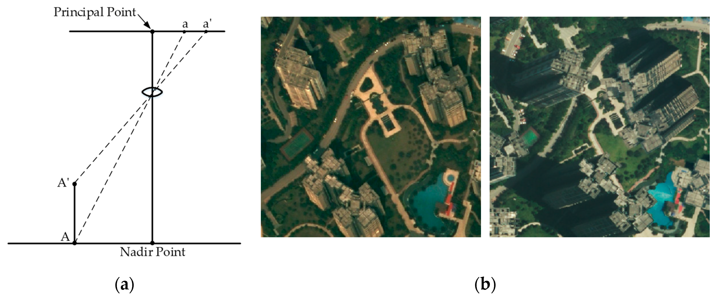
:1. Introduction
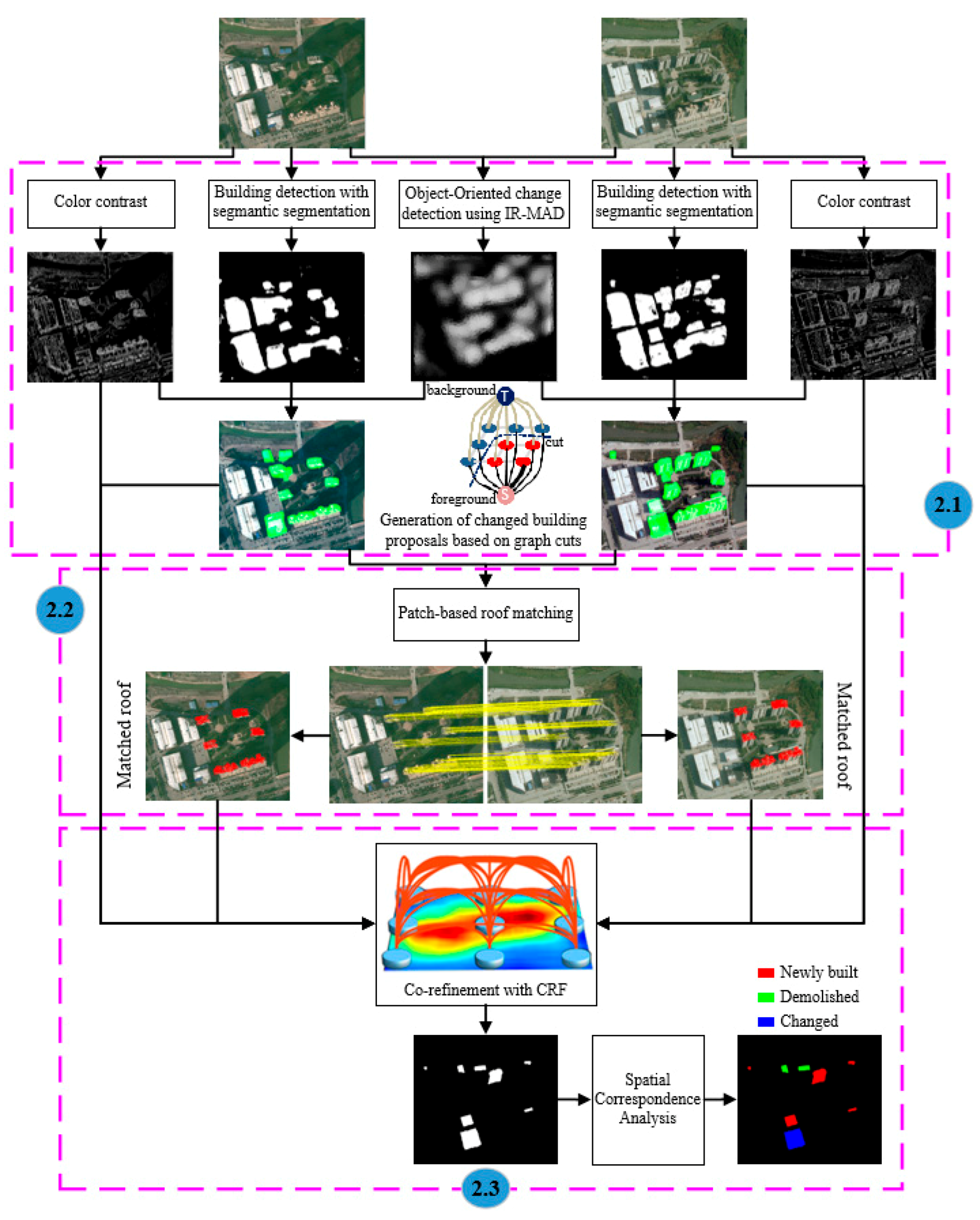
2. Methodology
2.1. Generation of Changed Building Proposals
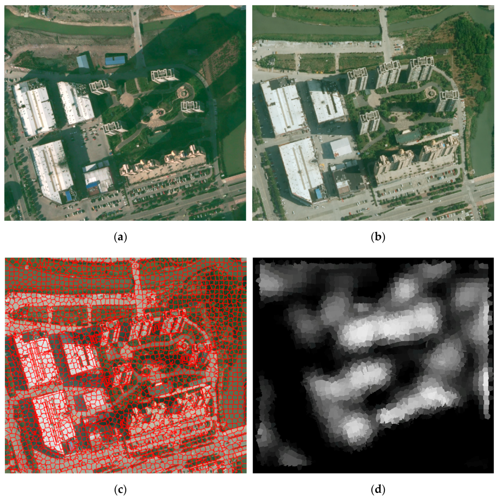
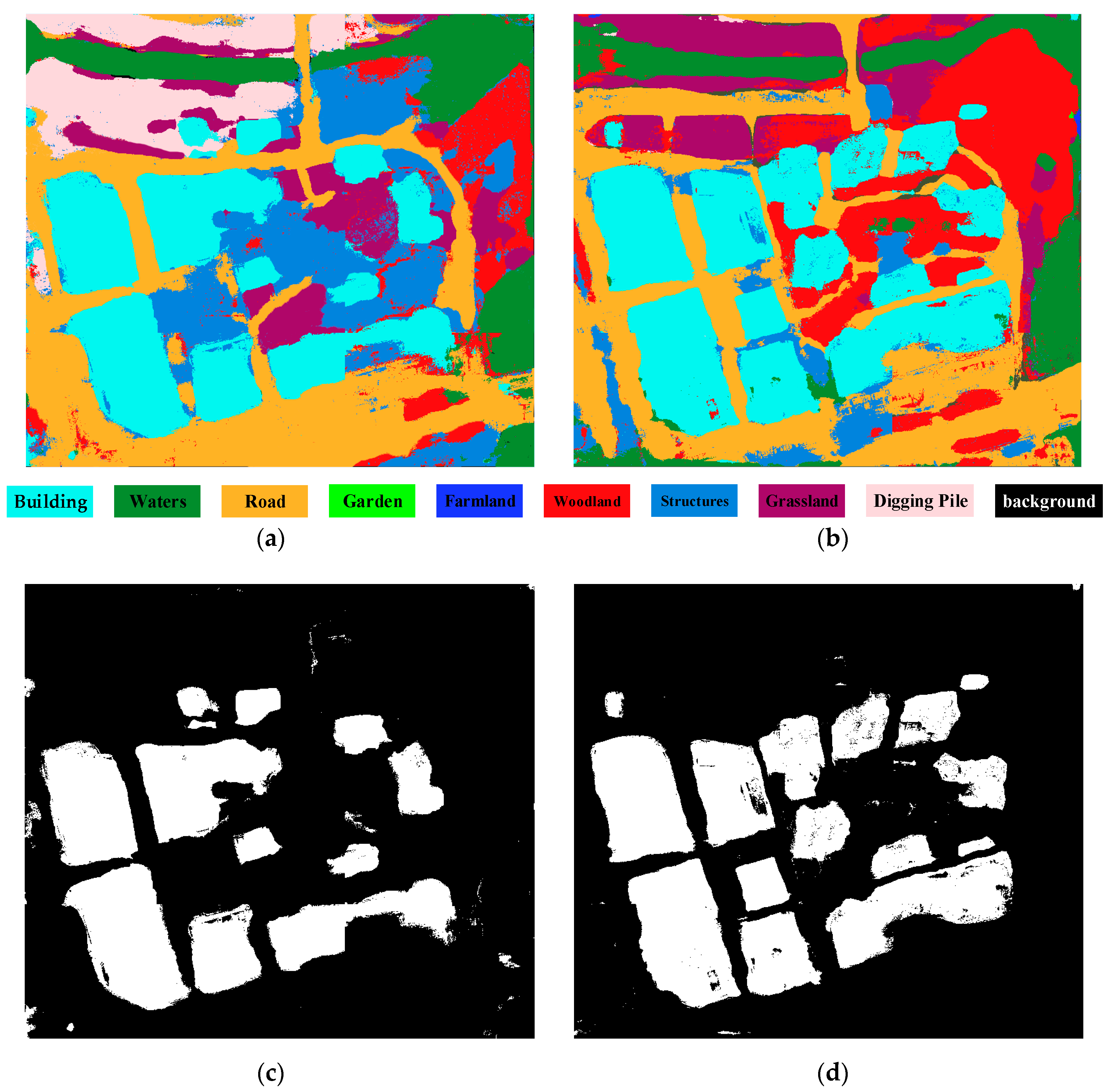
2.1.1. Object-Oriented Change Detection Using IR-MAD
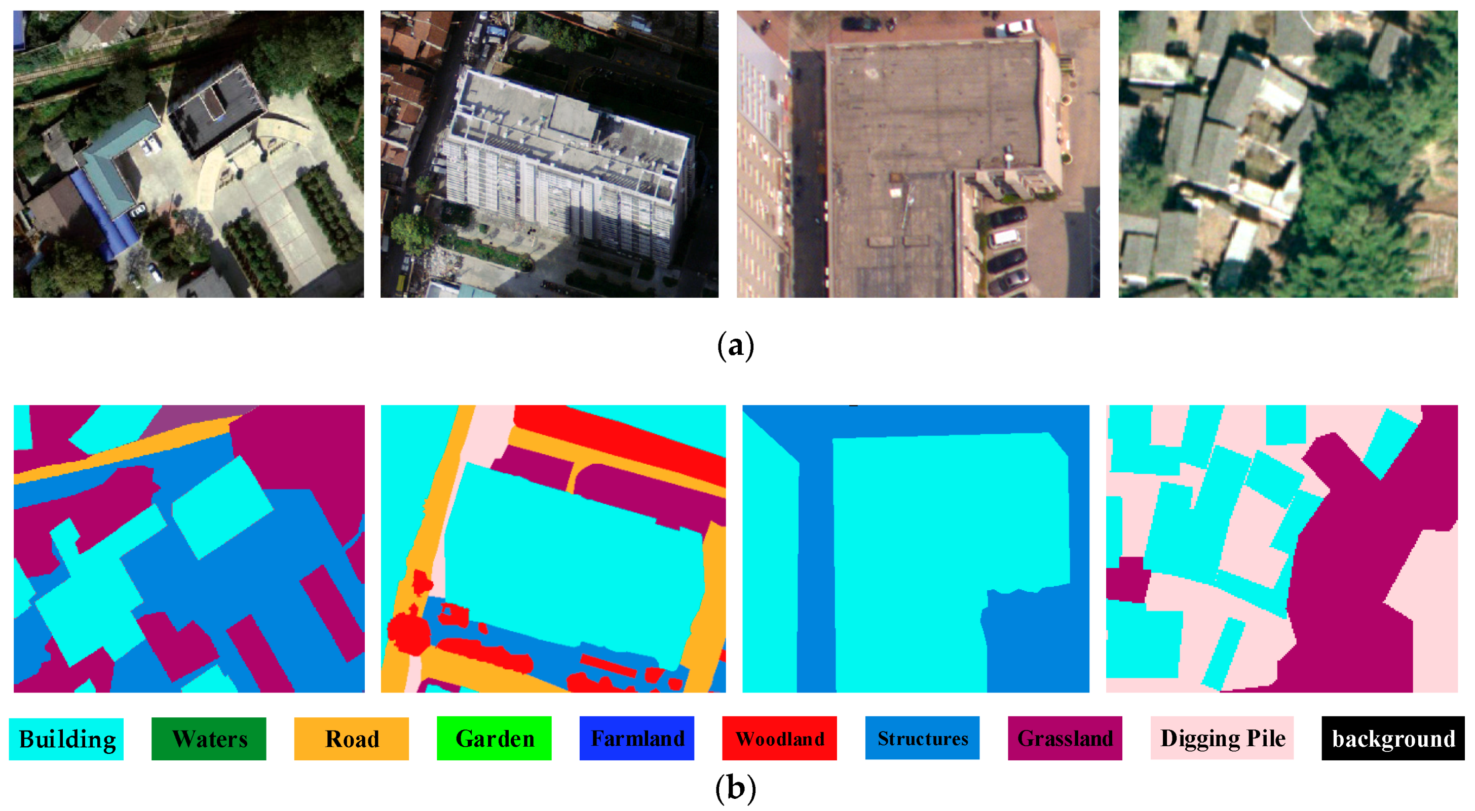
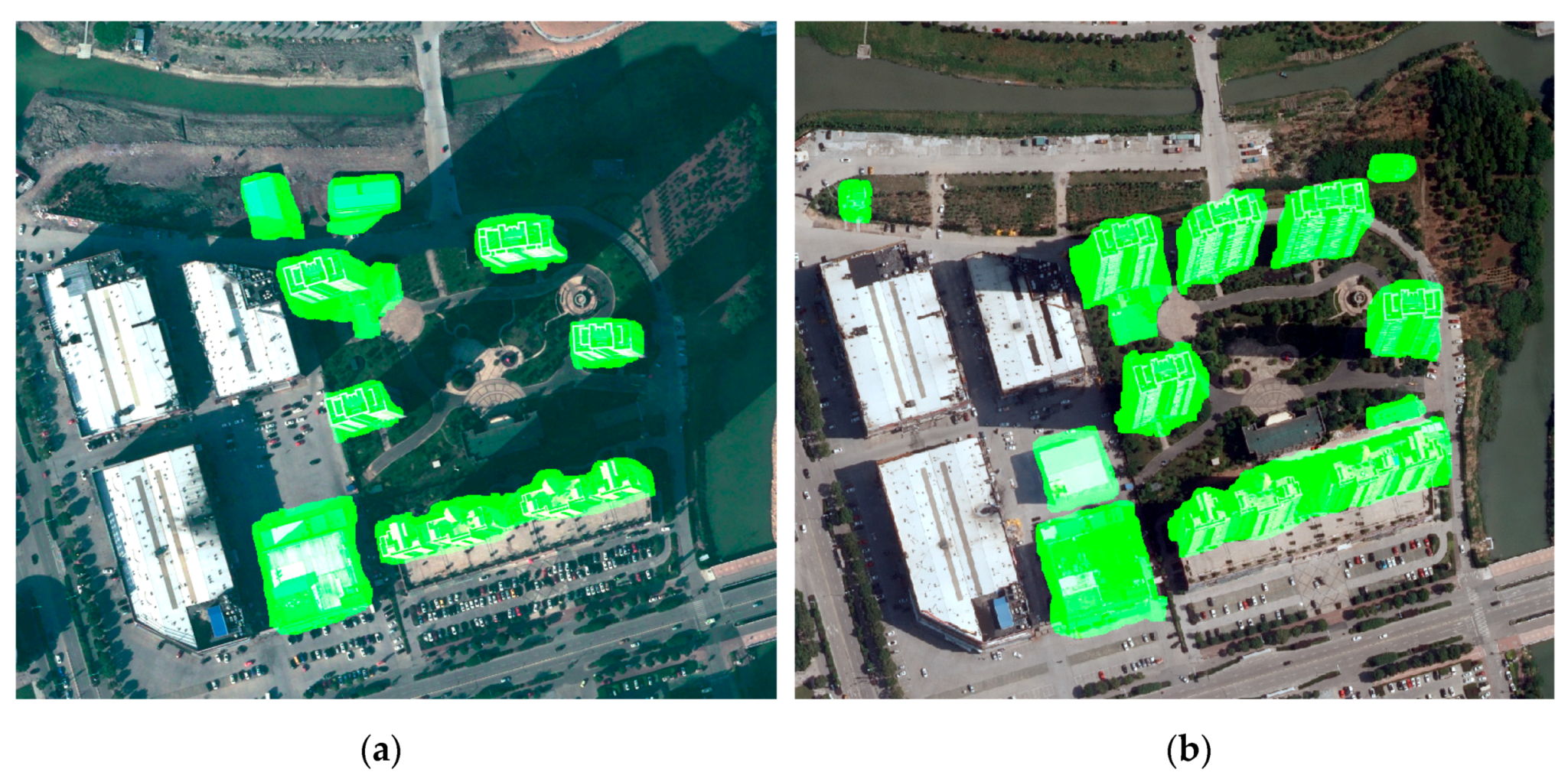
2.1.2. Building Extraction with Semantic Segmentation
2.1.3. Segmentation Based on Graph Cuts
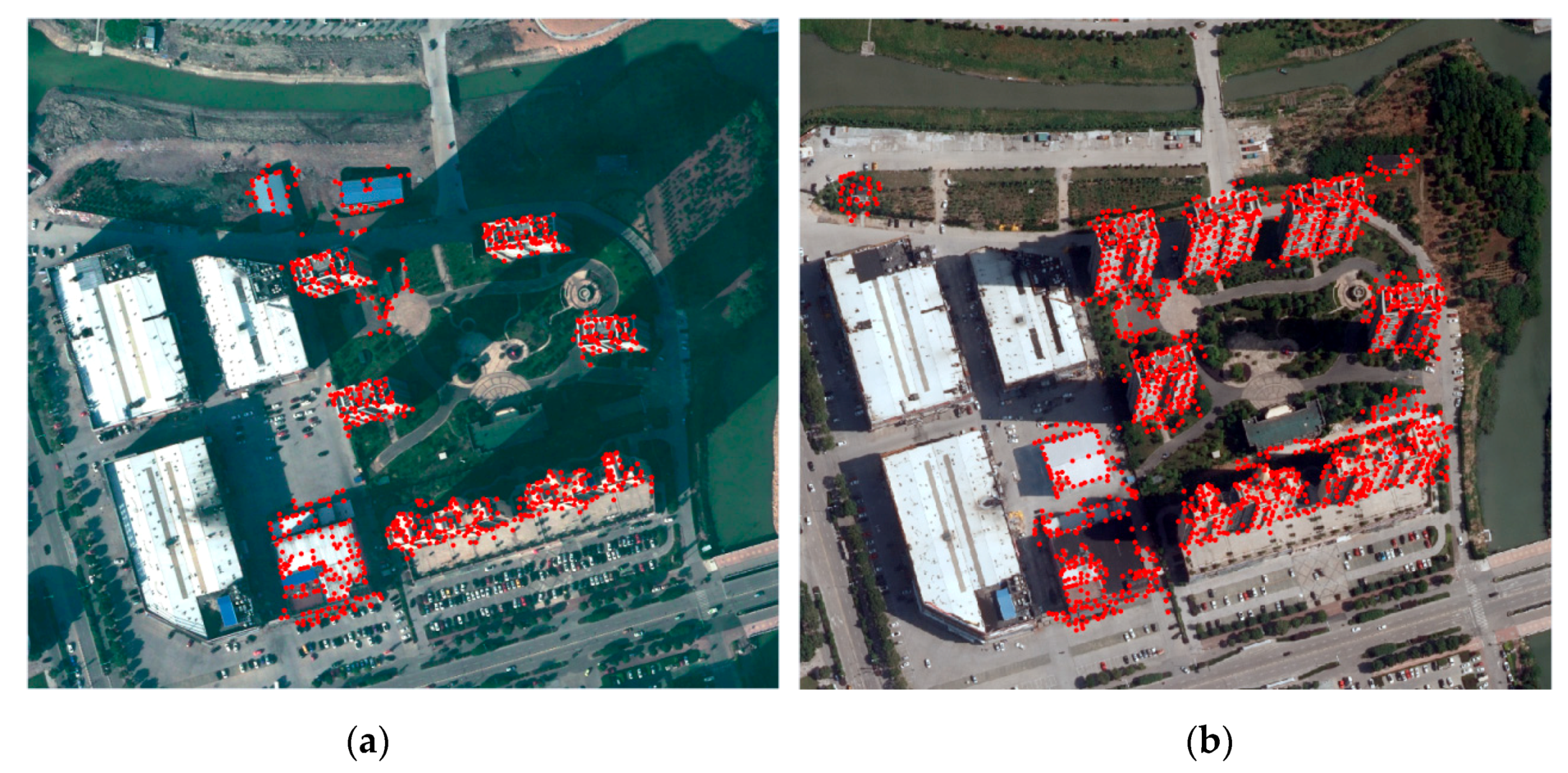
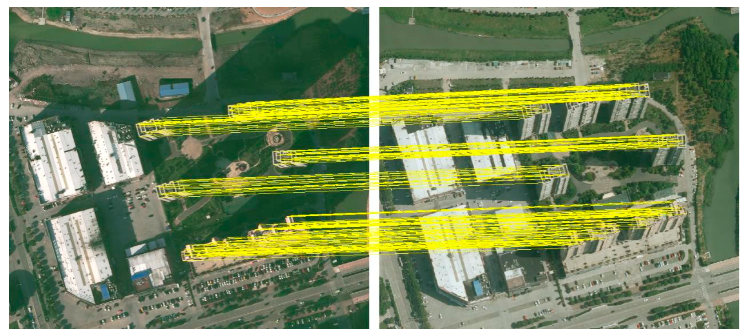
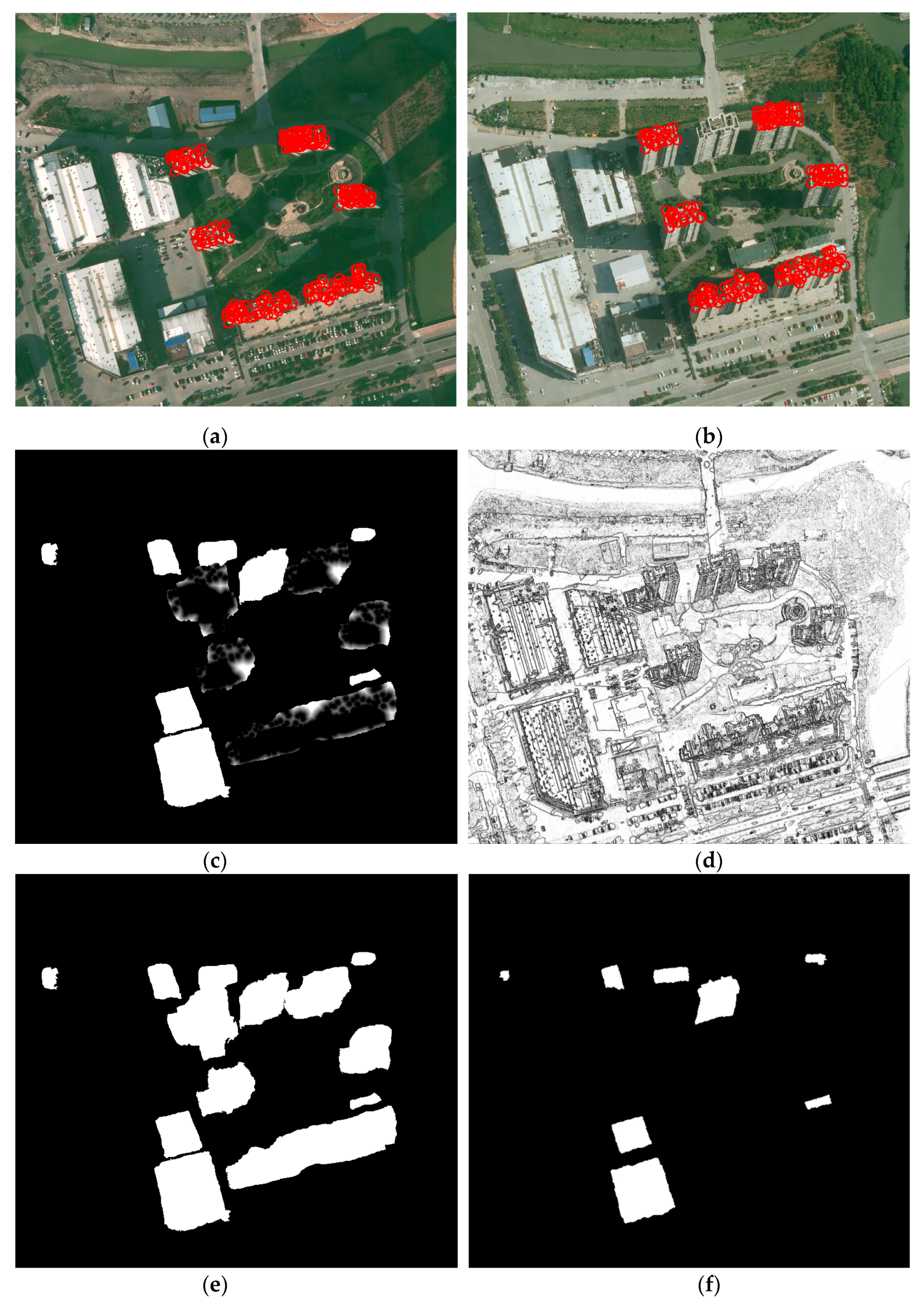
2.2. Patch-Based Matching
2.2.1. Feature Detection
2.2.2. Structural Feature Descriptor for Matching
2.3. Co-Refinement for Final Building Change Detection
2.3.1. Co-Refinement with CRF
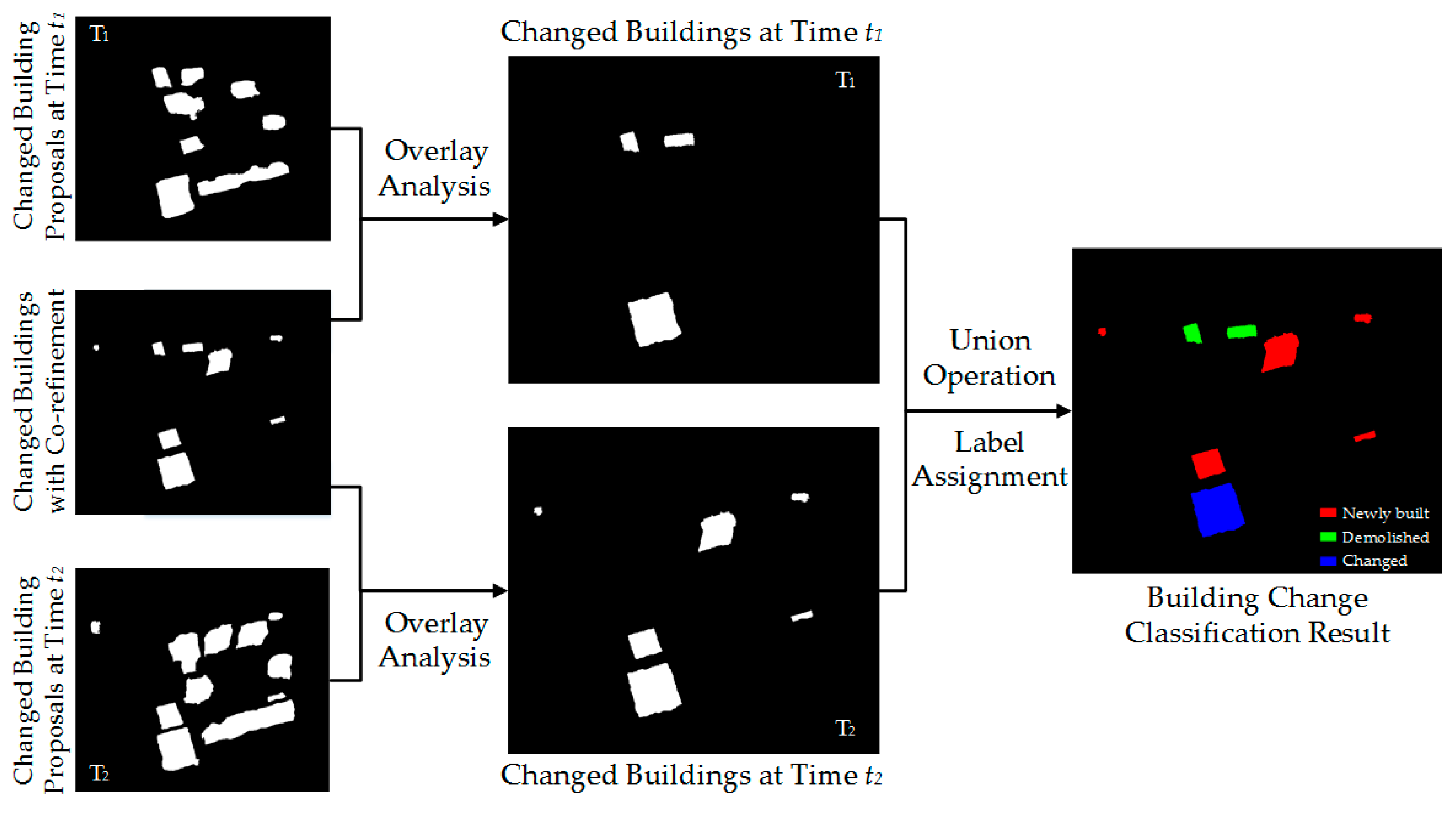
2.3.2. Type Identification of Changed Buildings
3. Experimental Results
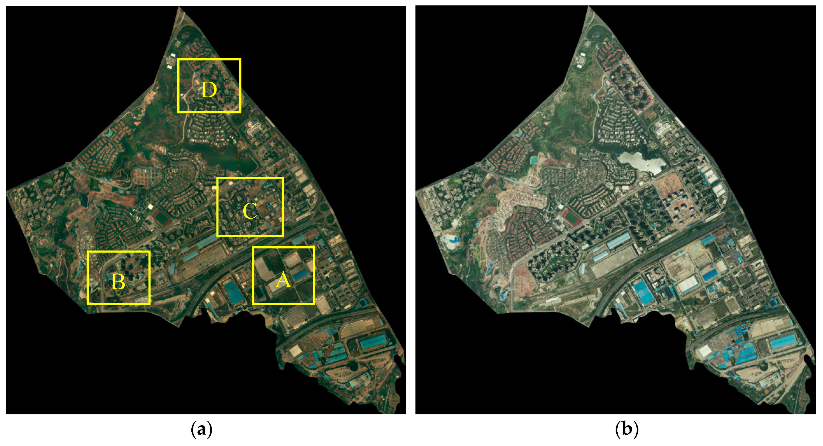
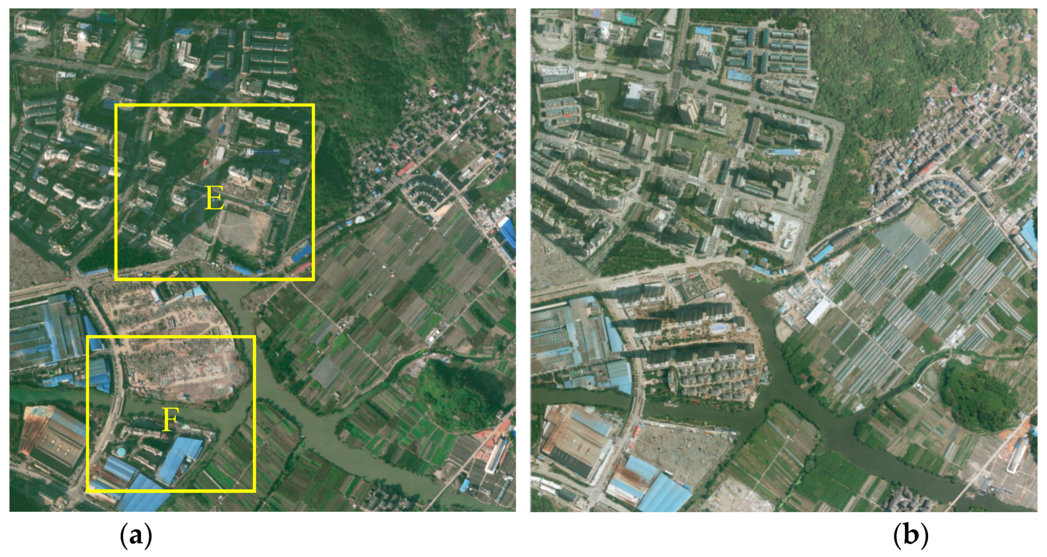
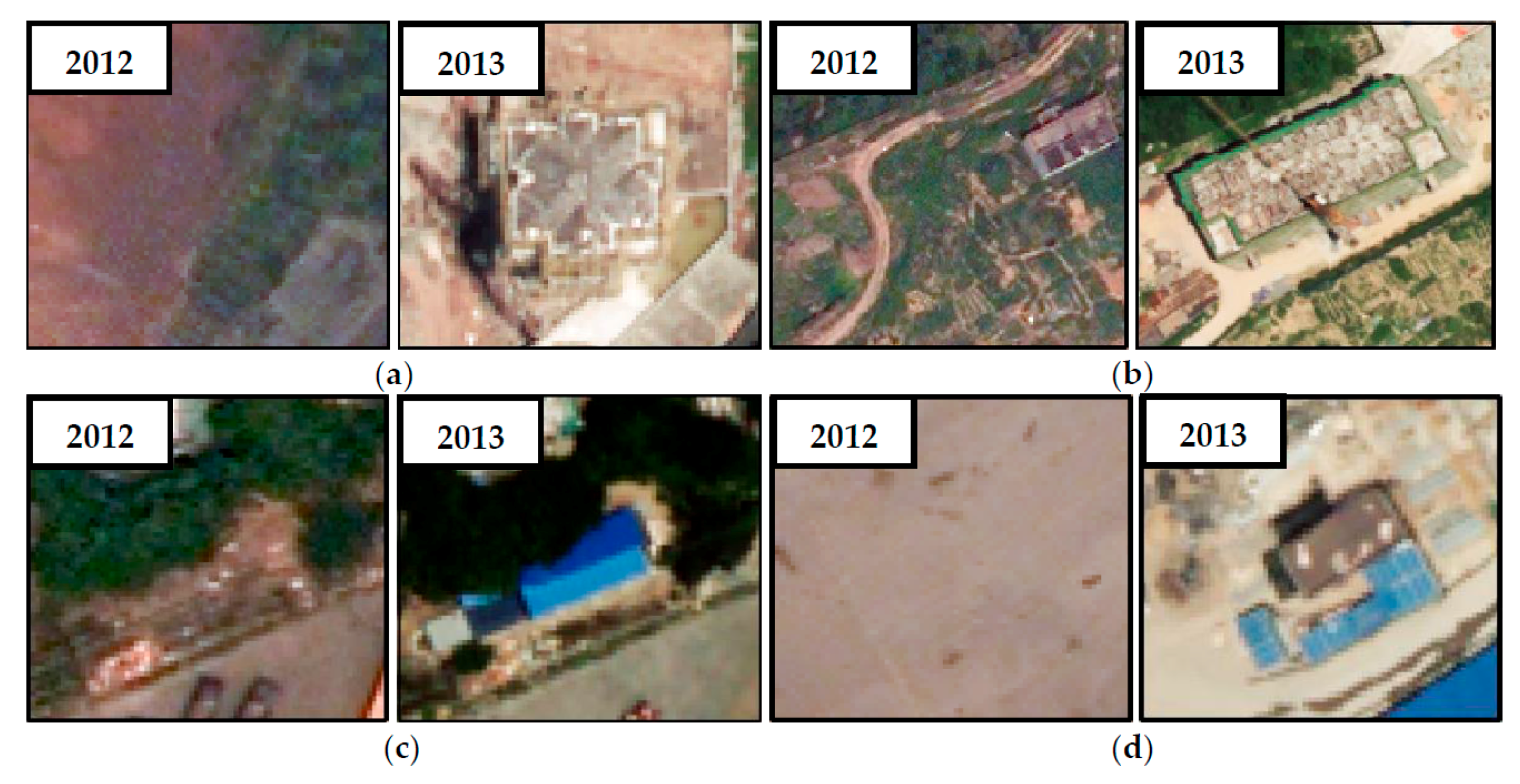
3.1. Study Site and Dataset Description
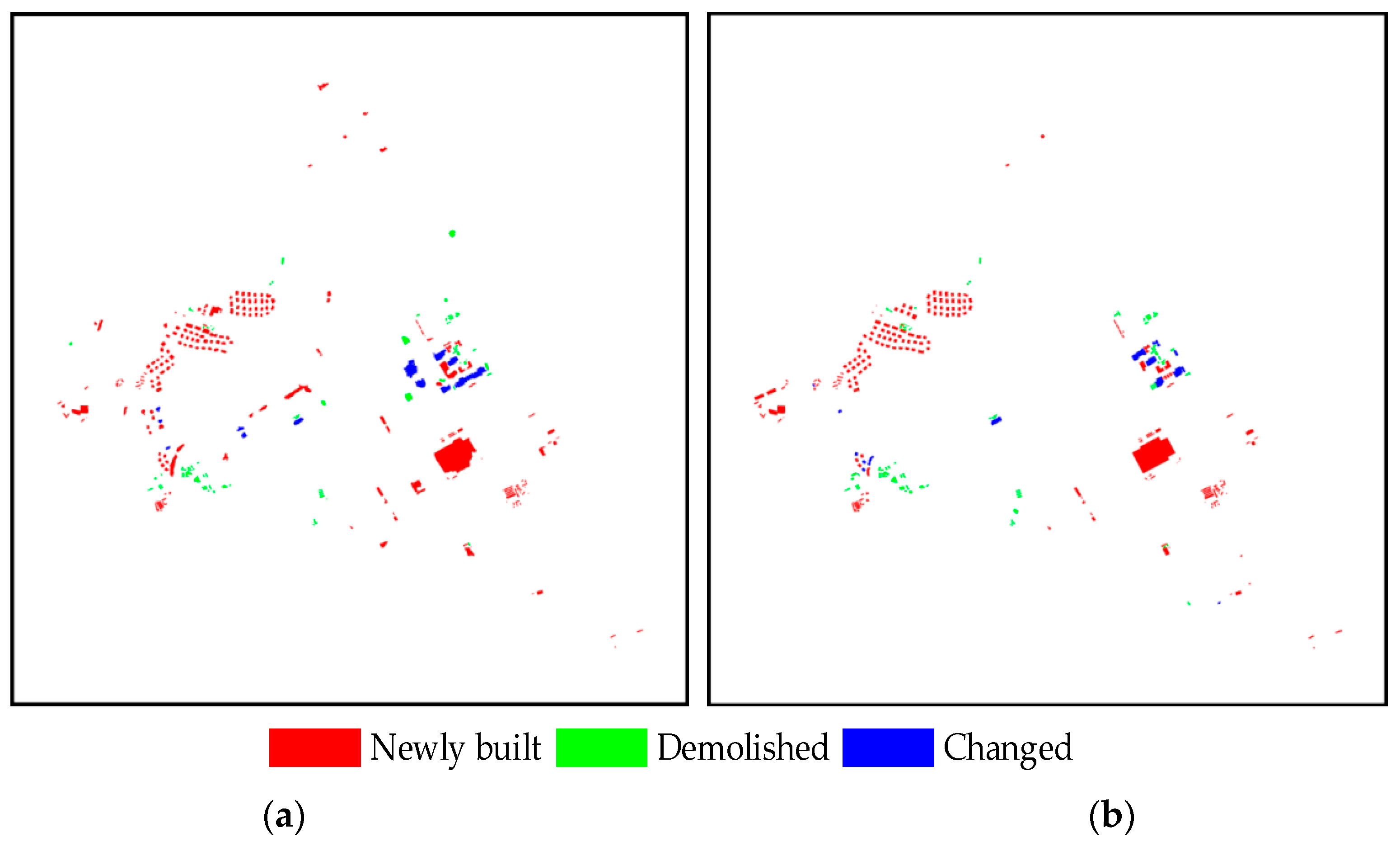
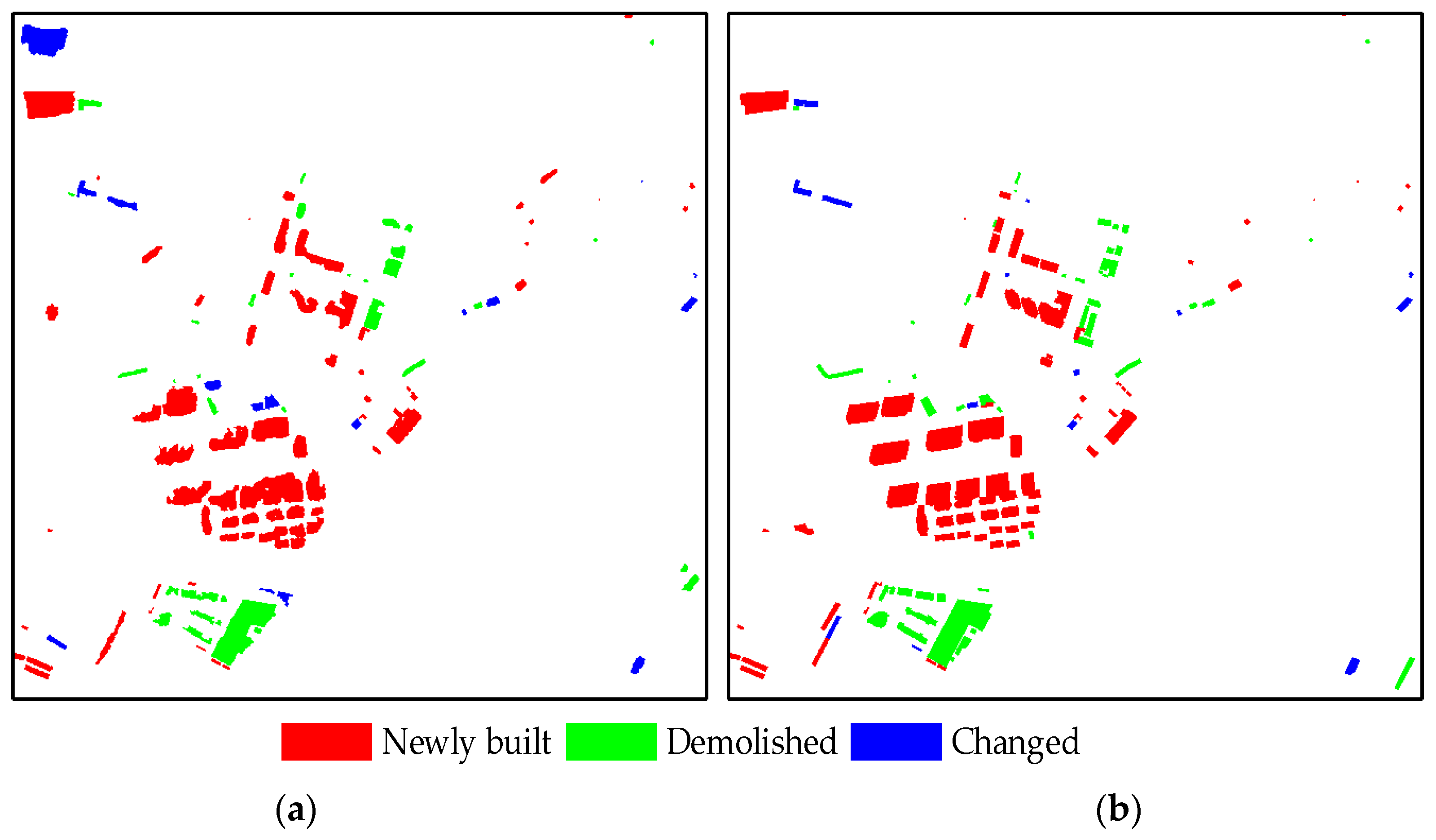
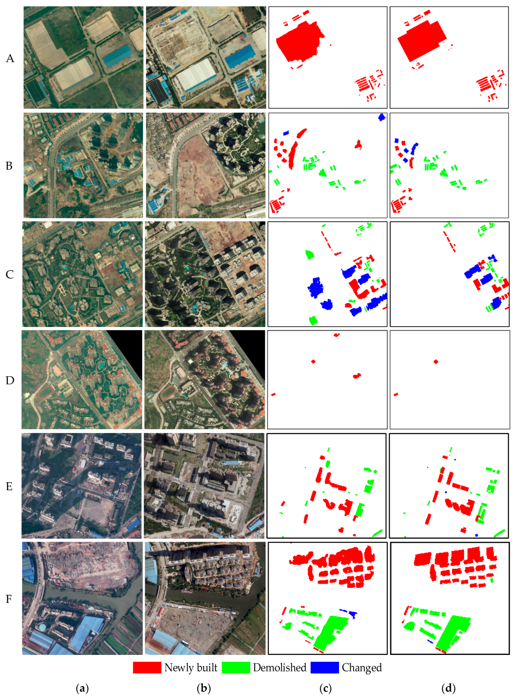
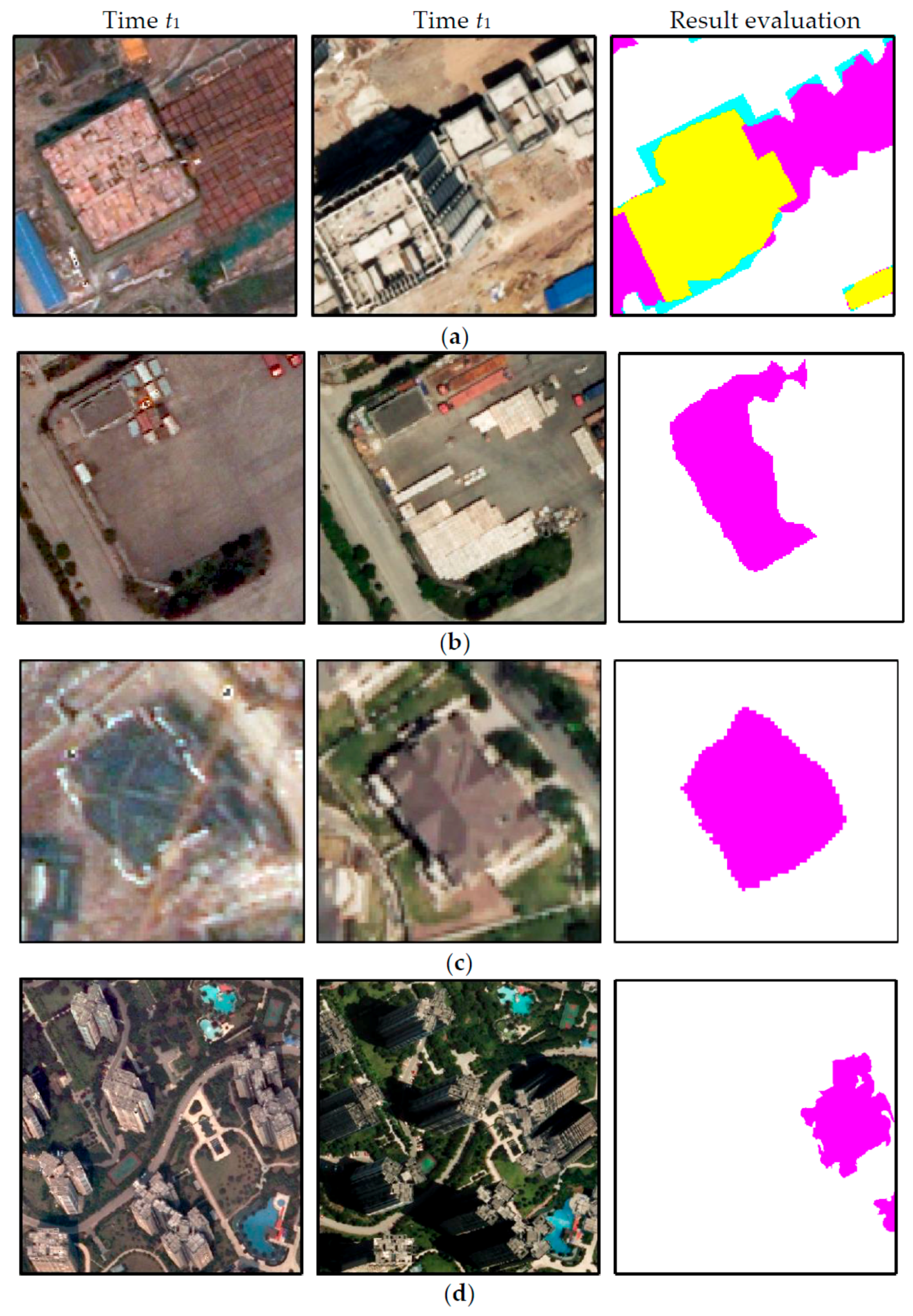
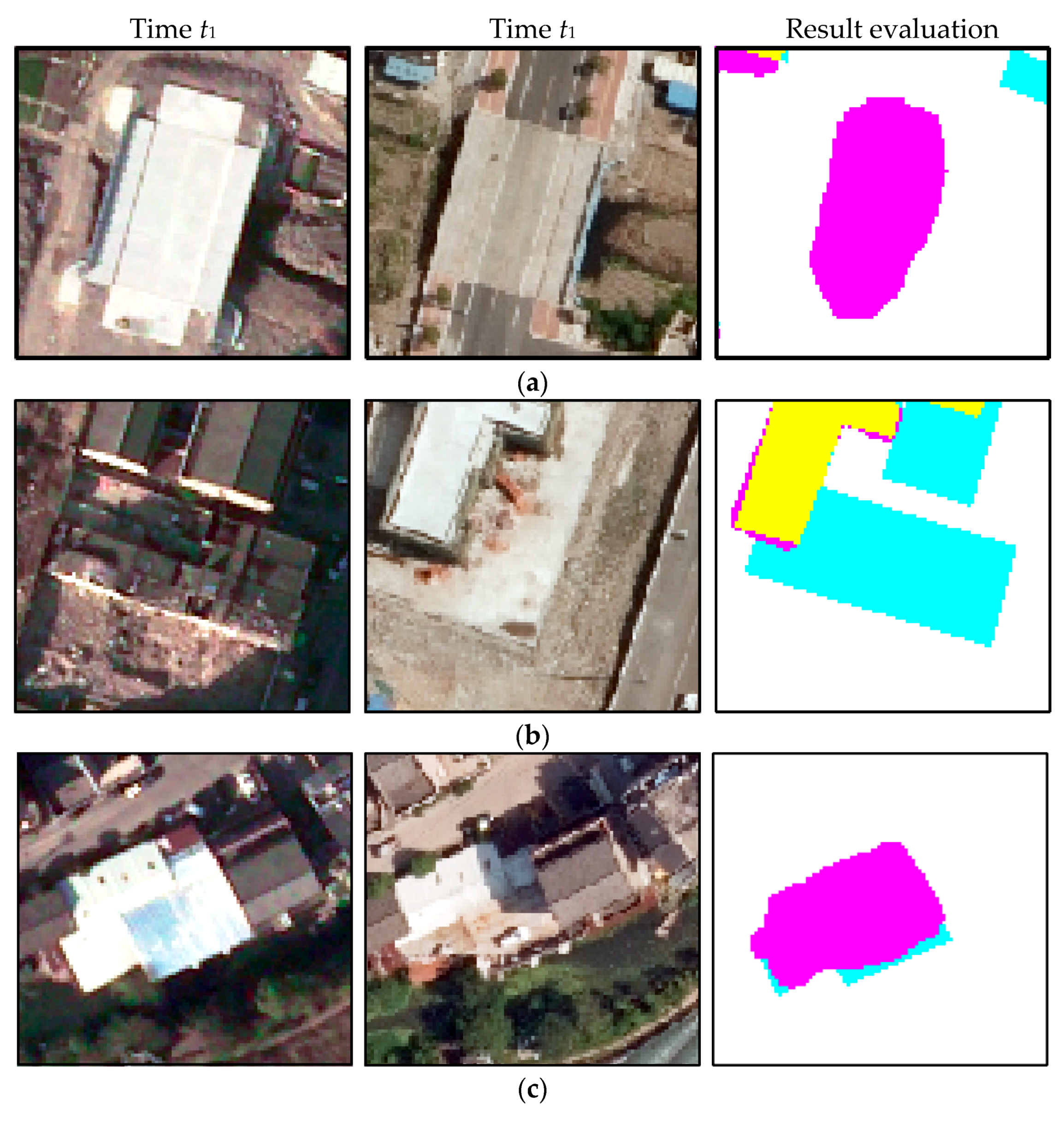
3.2. Building Change Detection Results
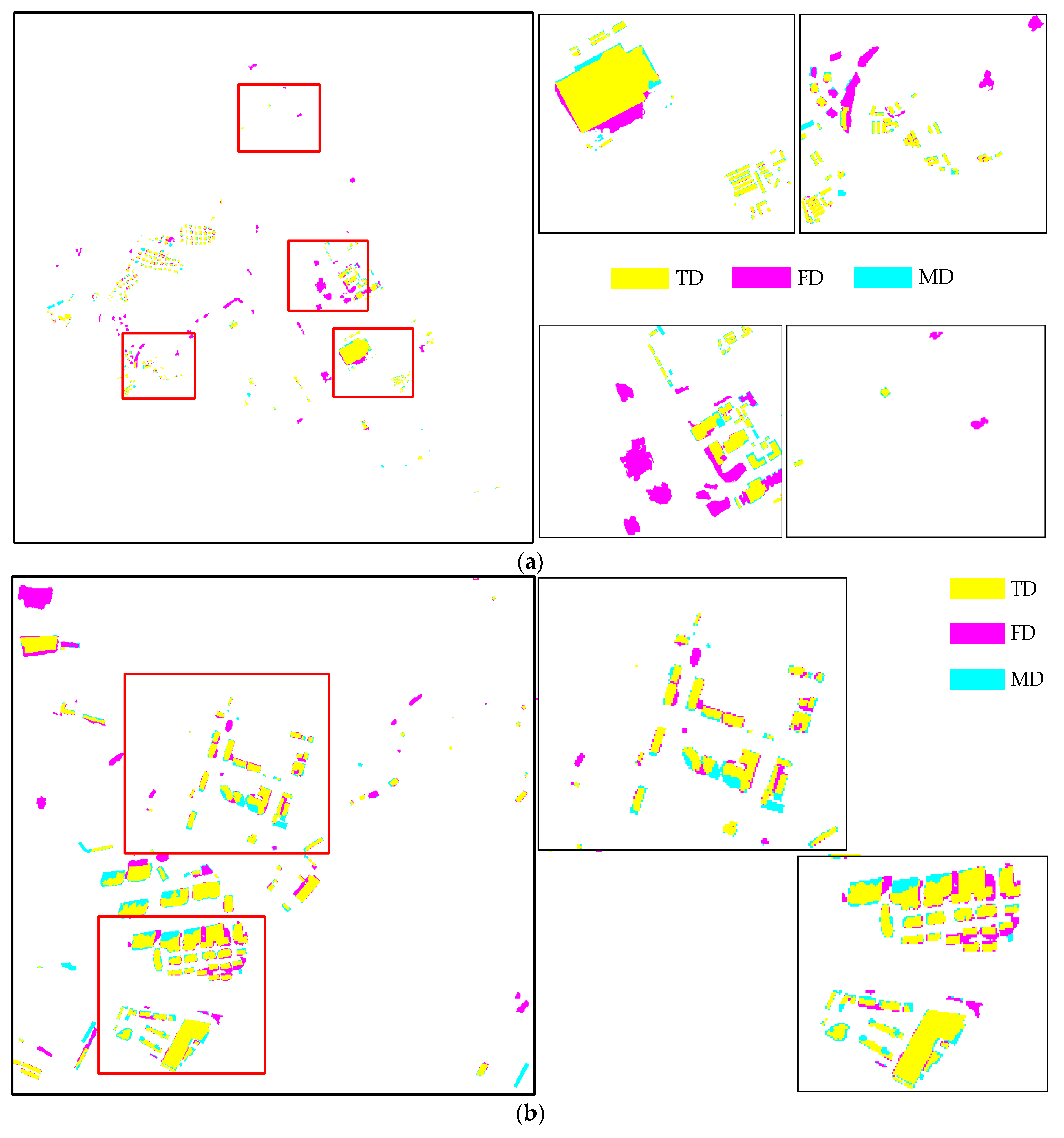
3.3. Quality Assessments
4. Discussion
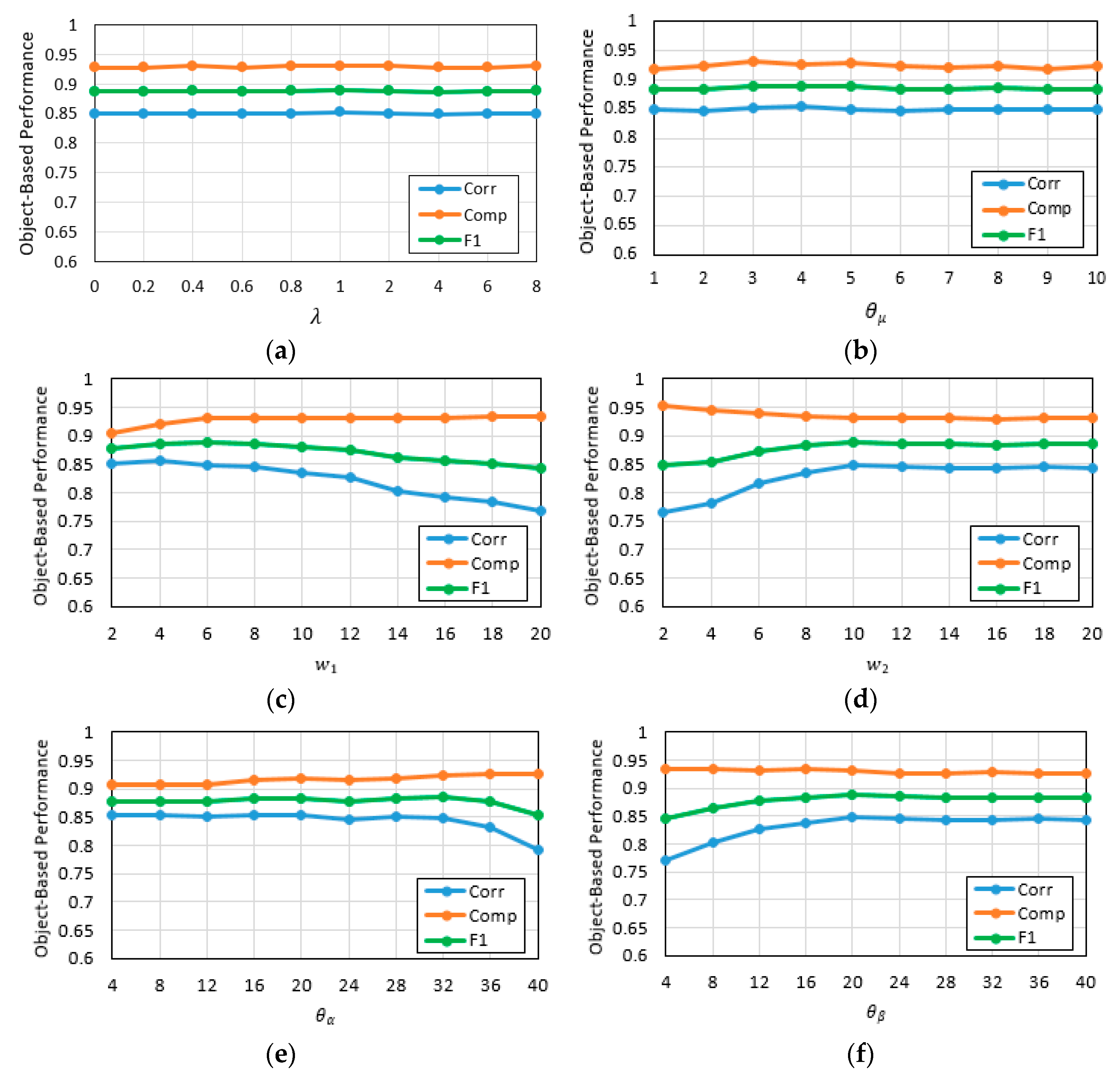
4.1. Parameter Selection
4.2. Advantages and Disadvantages of the Proposed Algorithm
5. Conclusions
Author Contributions
Funding
Acknowledgments
Conflicts of Interest
References
- Akçay, H.G.; Aksoy, S. Building Detection Using Directional Spatial Constraints. In Proceedings of the 2010 IEEE International Geoscience and Remote Sensing Symposium, Honolulu, HI, USA, 25–30 July 2010; pp. 1932–1935. [Google Scholar]
- Sofina, N.; Ehlers, M. Building Change Detection Using High Resolution Remotely Sensed Data and GIS. IEEE J. Sel. Top. Appl. Earth Obs. Remote Sens. 2017, 9, 3430–3438. [Google Scholar] [CrossRef]
- Gong, M.G.; Zhang, P.Z.; Su, L.; Liu, J. Coupled Dictionary Learning for Change Detection from Multisource Data. IEEE Trans. Geosci. Remote Sens. 2016, 54, 7077–7091. [Google Scholar] [CrossRef]
- Bruzzone, L.; Bovolo, F. A Novel Framework for the Design of Change Detection Systems for Very-high-resolution Remote Sensing Images. Proc. IEEE. 2013, 101, 609–630. [Google Scholar] [CrossRef]
- Bouziani, M.; Goïta, K.; He, D.-C. Automatic Change Detection of Buildings in Urban Environment from Very High Spatial Resolution Images Using Existing Geodatabase and Prior Knowledge. ISPRS J. Photogramm. Remote Sens. 2010, 65, 143–153. [Google Scholar] [CrossRef]
- Singh, A. Digital Change Detection Techniques Using Remotely-Sensed Data. Int. J. Remote Sens. 1989, 10, 989–1003. [Google Scholar] [CrossRef]
- Coppin, P.R.; Bauer, M.E. Digitial Change Detection in Forest Ecosystems with Remote Sensing Imagery. Remote Sens. Reviews. 1996, 13, 207–234. [Google Scholar] [CrossRef]
- Yuan, D.; Elvidge, C.D.; Lunetta, R.S. Survey of Multispectral Methods for Land Cover Change Analysis. In Remote Sensing Change Detection: Environmental Monitoring Methods and Applications; Lunetta, R.S., Elvidge, C.D., Eds.; Ann Arbor Press: Chelsea, MI, USA, 1998; pp. 21–39. [Google Scholar]
- Hecheltjen, A.; Thonfeld, F.; Menz, G. Recent Advances in Remote Sensing Change Detection—A Review. In Land Use and Land Cover Mapping in Europe; Manakos, I., Braun, M., Eds.; Springer: Dordrecht, The Netherlands, 2014; Volume 18, pp. 145–178. [Google Scholar]
- Chen, G.; Hay, G.J.; Carvalho, L.M.T.; Wulder, M.A. Object-based Change Detection. Int. J. Remote Sens. 2012, 33, 4434–4457. [Google Scholar] [CrossRef]
- Hussain, M.; Chen, D.; Cheng, A.; Wei, H.; Stanley, D. Change Detection from Remotely Sensed Images: From Pixel-Based to Object-Based Approaches. ISPRS J. Photogramm. Remote Sens. 2013, 80, 91–106. [Google Scholar] [CrossRef]
- Huang, X.; Zhu, T.T.; Zhang, L.P.; Tang, Y.Q. A Novel Buiding Change Index for Automatic Building Change Detection from High-resolution Remote Sensing Imagery. Remote Sens. Lett. 2014, 5, 713–722. [Google Scholar] [CrossRef]
- Tang, Y.; Huang, X.; Zhang, L. Fault-Tolerant Building Change Detection from Urban High-Resolution Remote Sensing Imagery. IEEE Geosci. Remote Sens. Lett. 2013, 10, 1060–1064. [Google Scholar] [CrossRef]
- Blaschke, T.; Hay, G.J.; Kelly, M.; Lang, S.; Hofmann, P.; Addink, E.; Queiroz Feitosa, R.; van der Meer, F.; van der Werff, H.; van Coillie, F.; et al. Geographic Object-based Image Analysis—Towards A New Paradigm. ISPRS J. Photogramm. Remote Sens. 2014, 87, 180–191. [Google Scholar] [CrossRef]
- Myint, S.W.; Gober, P.; Brazel, A.; Clark, S.G.; Weng, Q. Per-Pixel vs. Object-Based Classification of Urban Land Cover Extraction Using High Spatial Resolution Imagery. Remote Sens. Environ. 2011, 115, 1145–1161. [Google Scholar] [CrossRef]
- Sellaouti, A.; Wemmert, C.; Deruyver, A.; Hamouda, A. Template-based Hierarchical Building Extraction. IEEE Geosci. Remote Sens. Lett. 2013, 11, 706–710. [Google Scholar] [CrossRef]
- Xiao, P.; Yuan, M.; Zhang, X.; Feng, X.; Guo, Y. Cosegmentation for Object-Based Building Change Detection from High-resolution Remotely Sensed Images. IEEE Trans. Geosci. Remote Sens. 2017, 55, 1587–1603. [Google Scholar] [CrossRef]
- IM, J.; Jensen, J.; Tullis, J. Object-Based Change Detection Using Correlation Image Analysis and Image Segmentation. Int. J. Remote Sens. 2008, 29, 399–423. [Google Scholar] [CrossRef]
- Zhou, W.; Troy, A.; Grove, M. Object-Based Land Cover Classification and Change Analysis in the Baltimore Metropolitan Area Using Multitemporal High Resolution Remote Sensing Data. Sensors 2008, 8, 1613–1636. [Google Scholar] [CrossRef]
- Hou, B.; Wang, Y.; Liu, Q. A Saliency Guided Semi-Supervised Building Change Detection Method for High Resolution Remote Sensing Images. Sensors 2016, 16, 1377. [Google Scholar] [CrossRef]
- Huang, X.; Zhang, L.P.; Zhu, T.T. Buiding Change Detection from Multitemporal High-resolution Remotely Sensed Images Based on a Morphological Building Index. IEEE J. Sel. Top. Appl. Earth Obs. Remote Sens. 2014, 7, 105–115. [Google Scholar] [CrossRef]
- Huang, X.; Zhang, L.P. Morphological Building/Shadow Index for Building Extraction from High-resolution Imagery over Urban Area. IEEE J. Sel. Top. Appl. Earth Obs. Remote Sens. 2012, 5, 161–172. [Google Scholar] [CrossRef]
- Feng, T.; Shao, Z.F. Building Change Detection Based on the Enhanced Morphological Building Index. Sci. Surv. Mapp. 2017, 5, 237. [Google Scholar]
- Liu, H.F.; Yang, M.H.; Chen, J.; Hou, J.L.; Deng, M. Line-Constrained Shape Feature for Building Change Detection in VHR Remote Sensing Imagery. ISPRS Int. J. Geo-Inf. 2018, 7, 410. [Google Scholar] [CrossRef]
- Saito, S.; Yamashita, T.; Aoki, Y. Multiple Object Extraction from Aerial Imagery with Convolutional Neural Networks. J. Imaging Sci. Technol. 2016, 60, 1–9. [Google Scholar] [CrossRef]
- Gong, M.; Zhan, T.; Zhang, P.; Miao, Q. Superpixel-based difference representation learning for change detection in multispectral remote sensing images. IEEE Trans. Geosci. Remote Sens. 2017, 55, 2658–2673. [Google Scholar] [CrossRef]
- Daudt, R.C.; Saux, B.L.; Boulch, A.; Gousseau, Y. High Resolution Semantic Change Detection. arXiv, 2018; arXiv:1810.08452. [Google Scholar]
- Daudt, R.C.; Saux, B.L.; Boulch, A. Fully Convolutional Siamese Networks for Change Detection. arXiv, 2018; arXiv:1810.08462. [Google Scholar]
- Zhang, X.L.; Chen, X.W.; Li, F.; Yang, T. Change Detection Method for High Resolution Remote Sensing Images Using Deep Learning. Acta Geodaetica et Cartographica Sinica. 2017, 46, 999–1008. [Google Scholar]
- Zhou, Z.H.; Feng, J. Deep Forest: Towards an Alternative to Deep Neural Networks. arXiv, 2017; arXiv:1702.08835. [Google Scholar]
- Devi, S.; Veena. Measurement of Relief Displacement from Vertical Photograph. Int. J. Sci. Eng. Technol Res. 2014, 3, 2800–2805. [Google Scholar]
- Zhou, G.; Chen, W.; Kelmelis, J.A.; Zhang, D. A comprehensive study on urban true orthorectification. IEEE Trans. Geosci. Remote Sens. 2005, 43, 2138–2147. [Google Scholar] [CrossRef]
- Gong, J.Q.; Liu, Z.J.; Yan, Q.; Xu, Q.Q. Object-oriented island land cover change detection by iteratively reweighted multivariate statistical analysis. Marine Geodesy 2017, 40, 87–103. [Google Scholar] [CrossRef]
- Achanta, R.; Shaji, A.; Smith, K.; Lucchi, A.; Fua, P.; Süsstrunk, S. SLIC Superpixels Compared to State-of-the-Art Superpixel Methods. IEEE Trans. Pattern Anal. Mach. Intell. 2012, 34, 2274–2282. [Google Scholar] [CrossRef] [PubMed]
- Comaniciu, D.; Meer, P. Mean shift: A robust approach toward feature space analysis. IEEE Trans. Pattern Anal. Mach. Intell. 2002, 24, 603–619. [Google Scholar] [CrossRef]
- Beucher, S.; Mathmatique, C.D.M. The Watershed Transformation Applied to Image Segmentation. Scann. Microsc. Supp. 1991, 6, 299–314. [Google Scholar]
- Tewkesbury, A.P.; Comber, A.J.; Tate, N.J.; Lamb, A.; Fisher, P.F. A critical synthesis of remotely sensed optical image change detection techniques. Remote Sens. Environ. 2015, 160, 1–14. [Google Scholar] [CrossRef]
- Ojala, T.; Pietikäinen, M.; Mäenpää, T. Multiresolution Gray-Scale and Rotation Invariant Texture Classification with Local Binary Patterns. IEEE Trans. Pattern Anal. Mach. Intell. 2002, 24, 971–987. [Google Scholar] [CrossRef]
- Ma, W.Y.; Manjunath, B.S. Texture Features and Learning Similarity. In Proceedings of the IEEE Computer Society Conference on Computer Vision and Pattern Recognition, San Francisco, CA, USA, 18–20 June 1996; pp. 425–430. [Google Scholar]
- Canty, M.J.; Nielsen, A.A. Investigation of alternative iteration schemes for the IR-MAD algorithm. In Proceedings of the International Society for Optical Engineering, Bellingham, WA, USA, 1 January 2007; pp. 8–10. [Google Scholar]
- Nielsen, A.A.; Canty, M.J. Multi- and hyperspectral remote sensing change detection with generalized difference images by the IR-MAD method. In Proceedings of the International Workshop on Analysis of Multi-temporal Remote Sensing Images, Biloxi, MS, USA, 16–18 May 2005; pp. 69–173. [Google Scholar]
- Zhang, M.; Hu, X.; Zhao, L.; Lv, Y.; Luo, M.; Pang, S. Learning dual multi-scale manifold ranking for semantic segmentation of high-resolution images. Remote Sens. 2017, 9, 500. [Google Scholar] [CrossRef]
- Boykov, Y. Interactive graph cuts for optimal boundary and region segmentation of objects in N-D images. In Proceedings of the 8th IEEE International Conference on Computer Vision (ICCV), Vancouver, BC, Canada, 7–14 July 2001; pp. 105–112. [Google Scholar]
- Boykov, Y.; Kolmogorov, V. An experimental comparison of min-cut/max-flow algorithms for energy minimization in vision. IEEE Trans. Pattern Anal. Mach. Intell. 2004, 26, 1124–1137. [Google Scholar] [CrossRef] [PubMed]
- Papadopoulos, D.P.; Uijlings, J.R.R.; Keller, F.; Ferrari, V. Extreme clicking for efficient object annotation. In Proceedings of the IEEE International Conference on Computer Vision, Venice, Italy, 22–29 October 2017; pp. 4940–4949. [Google Scholar]
- Rother, C.; Kolmogorov, V.; Blake, A. “GrabCut”: Interactive foreground extraction using iterated graph cuts. ACM Siggraph. 2004, 23, 309–314. [Google Scholar] [CrossRef]
- Morrone, M.C.; Owens, R.A. Feature Detection from Local Energy. Pattern Recogn. Lett. 1987, 6, 303–313. [Google Scholar] [CrossRef]
- Field, D.J. Relations between the statistics of natural images and the response properties of cortical cells. J. Opt. Soc. Am. A. 1987, 4, 2379–2394. [Google Scholar] [CrossRef] [PubMed]
- Kovesi, P. Phase Congruency: A Low-Level Image Invariant. Psycholog. Res. 2000, 64, 136–148. [Google Scholar] [CrossRef]
- Horn, B.K.P. Robot Vision; MIT press: Cambridge, MA, USA, 1986. [Google Scholar]
- Li, J.; Hu, Q.; Ai, M. RIFT: Multi-modal Image Matching Based on Radiation-Invariant Feature Transform. arXiv, 2018; arXiv:1804.09493. [Google Scholar]
- Kovesi, P.D. Phase Congruency Detects Corners and Edges. In Proceedings of the 7th International Conference on Digital Image Computing: Techniques and Applications, Sydney, Australia, 10–12 December 2003; pp. 309–318. [Google Scholar]
- Ye, Y.; Shan, J.; Bruzzone, L.; Shen, L. Robust registration of multimodal remote sensing images based on structural similarity. IEEE Trans. Geosci. Remote Sens. 2017, 55, 2941–2958. [Google Scholar] [CrossRef]
- Krähenbühl, P.; Koltun, V. Efficient Inference in Fully Connected CRFs with Gaussian Edge Potentials. arXiv, 2012; arXiv:1210.5644. [Google Scholar]
- Cheng, M.M.; Prisacariu, V.A.; Zheng, S.; Torr, P.; Rother, C. DenseCut: Densely Connected CRFs for Realtime GrabCut. Comput. Graphics Forum 2015, 34, 193–201. [Google Scholar] [CrossRef]
- Özdemir, B.; Aksoy, S.; Eckert, S.; Pesaresi, M.; Ehrlich, D. Performance measures for object detection evaluation. Pattern Recogn. Lett. 2010, 31, 1128–1137. [Google Scholar] [CrossRef]
- Ok, A.O.; Senaras, C.; Yuksel, B. Automated Detection of Arbitrarily Shaped Buildings in Complex Environments from Monocular VHR Optical Satellite Imagery. IEEE Trans. Geosci. Remote Sens. 2013, 51, 1701–1717. [Google Scholar] [CrossRef]

| Time t1/Time t2 | Changed Building | No Building Change |
|---|---|---|
| Changed Building | Changed | Demolished |
| No building change | Newly built | No building change |
| Analyzed Dataset | Proposed/Ground Truth | No. Building Change | Newly Built | Demolished | Changed |
|---|---|---|---|---|---|
| Dataset 1 | No Building Change | 0 | 13 | 9 | 2 |
| Newly Built | 24 | 212 | 1 | 7 | |
| Demolished | 6 | 0 | 82 | 2 | |
| Changed | 8 | 4 | 2 | 5 | |
| Dataset 2 | No Building Change | 0 | 6 | 4 | 1 |
| Newly Built | 8 | 71 | 0 | 3 | |
| Demolished | 5 | 0 | 47 | 2 | |
| Changed | 4 | 2 | 3 | 9 |
| Analyzed Dataset | No. of Correctly Detected Buildings | No. of Wrongly Detected Buildings | Corr (%) | Comp (%) | F1 (%) | |
|---|---|---|---|---|---|---|
| TD | FD | MD | ||||
| Dataset 1 | 299 | 54 | 24 | 84.70 | 92.57 | 88.46 |
| Dataset 2 | 127 | 27 | 11 | 82.46 | 92.03 | 86.98 |
© 2019 by the authors. Licensee MDPI, Basel, Switzerland. This article is an open access article distributed under the terms and conditions of the Creative Commons Attribution (CC BY) license (http://creativecommons.org/licenses/by/4.0/).
Share and Cite
Gong, J.; Hu, X.; Pang, S.; Li, K. Patch Matching and Dense CRF-Based Co-Refinement for Building Change Detection from Bi-Temporal Aerial Images. Sensors 2019, 19, 1557. https://doi.org/10.3390/s19071557
Gong J, Hu X, Pang S, Li K. Patch Matching and Dense CRF-Based Co-Refinement for Building Change Detection from Bi-Temporal Aerial Images. Sensors. 2019; 19(7):1557. https://doi.org/10.3390/s19071557
Chicago/Turabian StyleGong, Jinqi, Xiangyun Hu, Shiyan Pang, and Kun Li. 2019. "Patch Matching and Dense CRF-Based Co-Refinement for Building Change Detection from Bi-Temporal Aerial Images" Sensors 19, no. 7: 1557. https://doi.org/10.3390/s19071557
APA StyleGong, J., Hu, X., Pang, S., & Li, K. (2019). Patch Matching and Dense CRF-Based Co-Refinement for Building Change Detection from Bi-Temporal Aerial Images. Sensors, 19(7), 1557. https://doi.org/10.3390/s19071557