COSMOS: Collaborative, Seamless and Adaptive Sentinel for the Internet of Things


Abstract
1. Introduction
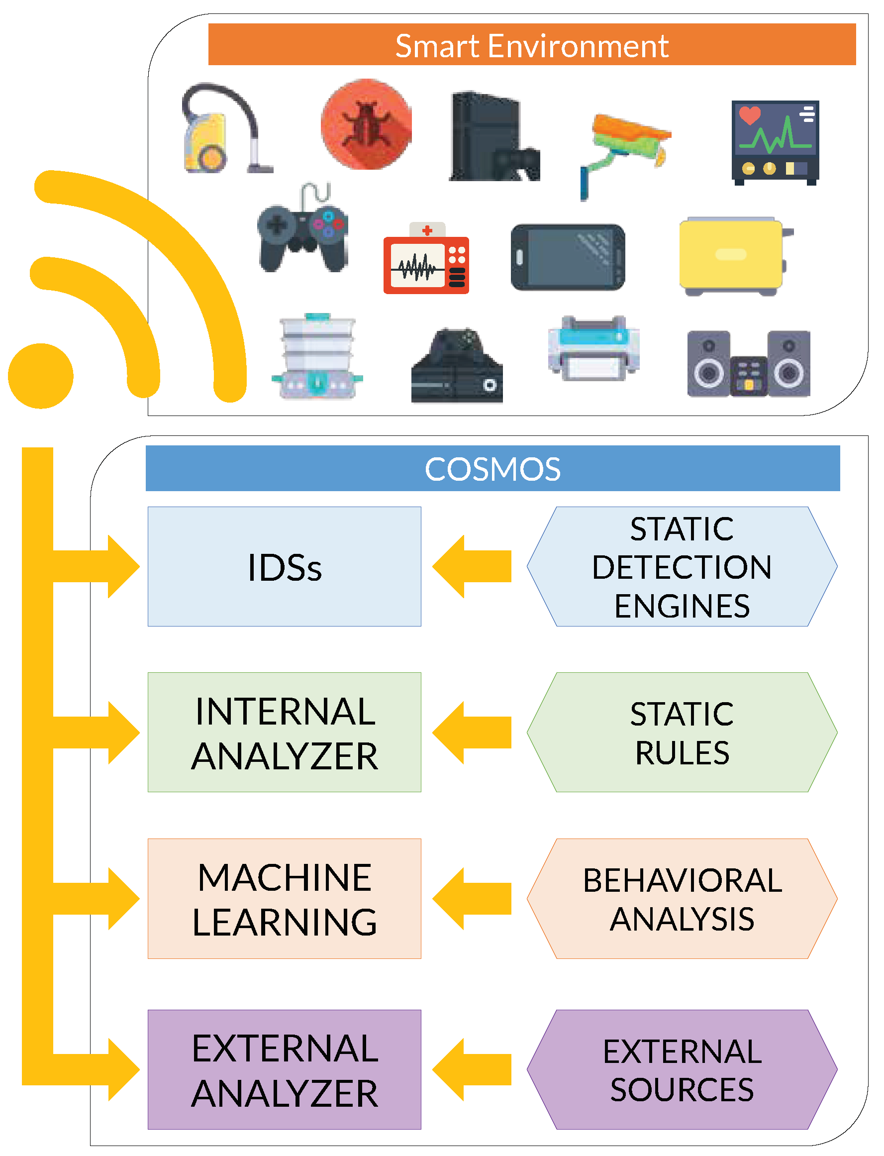
- The proposal of COSMOS (see Figure 1) based on a defense-in-depth approach oriented to perform the main security functions for asset protection (identify, protect, detect, react and recover) within an IoT ecosystem.
- The design of a mechanism for sharing threat intelligence between IoT Sentinels, which is critical to guarantee collaboration, reduce incidents’ response time and prevent attacks.
- The conception of an adaptive mechanism that allows for updating defense capabilities in IoT Sentinels, making them resilient to an evolutionary threat environment.
- The development and evaluation of COSMOS as a full-fledged security framework aiming to be as much seamless as possible to users, automatic, portable, easy to deploy and manageable in a pragmatic way through a mobile application.
2. Collaborative, Seamless and Adaptive IoT Sentinel
- Offer essential security services: COSMOS should provide a set of essential security services for IoT devices, i.e., identify those IoT devices to be protected, deploy security countermeasures to protect them, detect attack attempts, react automatically to incidents and recover the normal operation of the IoT ecosystem.
- Share threat intelligence: Design a collaboration mechanism between IoT sentinels allowing for sharing threat intelligence information which can be useful in the treatment of security incidents and help to prevent IoT attacks.
- Adapt to the threat environment: Develop a mechanism to make COSMOS adaptive within continuously evolving threat environments, making it resilient against threats that have been detected in the past by another IoT Sentinel [22].
- Follow a psychological acceptability approach: The implementation of the proposal should provide transparency to the users of the framework, automation of operation, portability, easiness of deployment and management in a pragmatic way.
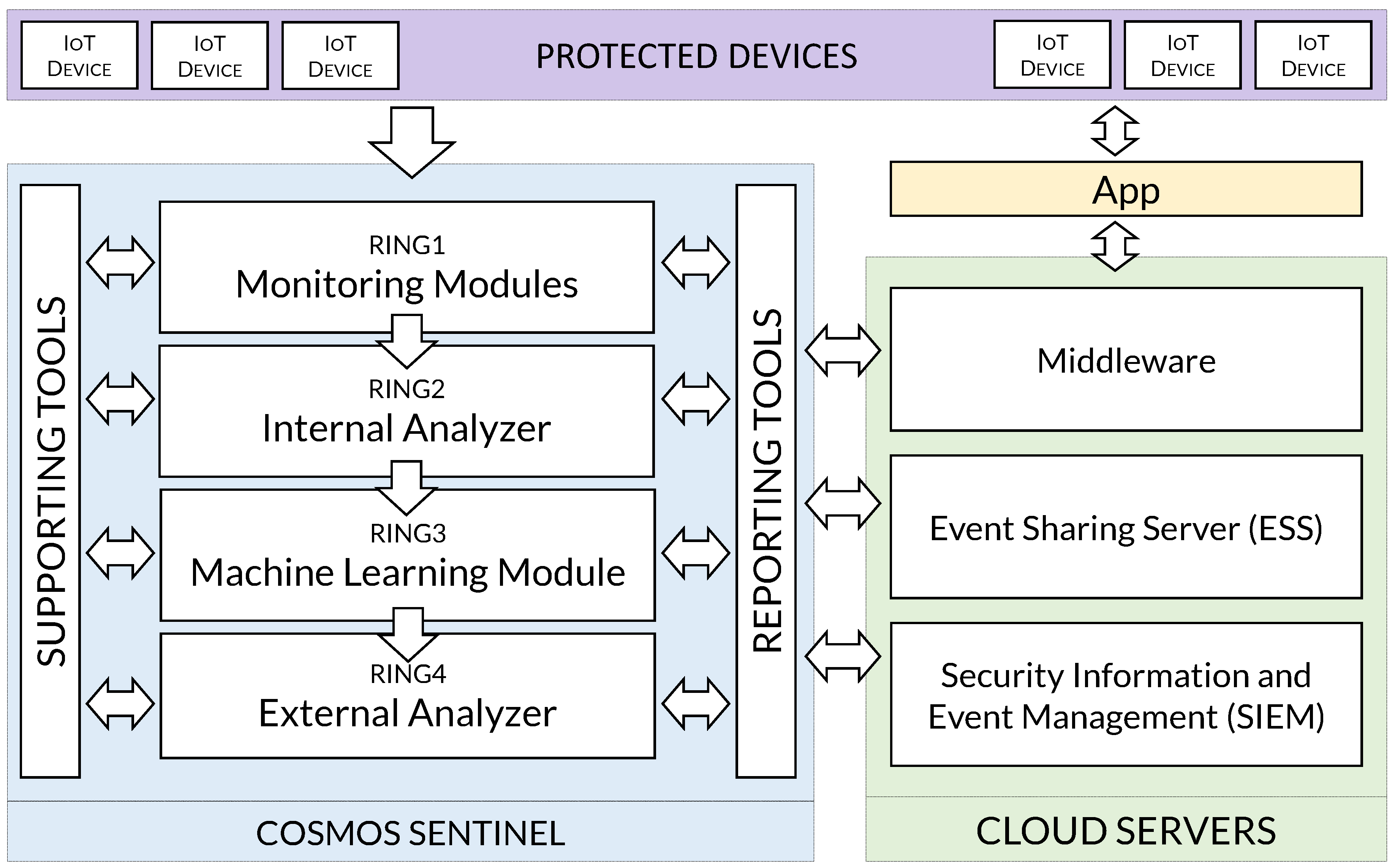
2.1. Monitoring Modules
2.2. Analyzer Modules
2.3. Supporting Tools
2.4. Reporting Tools
2.5. Cloud Servers
3. IoT Sentinel Use Cases
3.1. Case 1: Suspicious Frame Detected by the Monitoring Modules
3.2. Case 2: Suspicious File Classified as Malware by the Internal Analyzer
3.3. Case 3: Suspicious File Classified as Malware by the Machine Learning Module
3.4. Case 4: Suspicious File Classified as Malware by the External Analyzer
3.5. Case 5: Suspicious File Classified as Goodware by the Detection Layers
4. Experiments
4.1. Testing COSMOS Capabilities as an Intrusion Detector
4.1.1. Settings
- Raspberry Pi 3 Model B uses the Raspbian OS with the Linux kernel version 4.1.19, Snort version 2.9.8.0 and Kismet version 2016-01-R1. The Sentinel performed the detection duties using two wireless interfaces: the Pi built-in WLAN chip communicated with OSSIM through Rsyslog, and an external Alfa AWUS036H USB antenna sniffed wireless traffic in the surrounding area.
- Laptop running a Kali 2.0 distribution, used for penetration testing [45], with Linux kernel version 4.3.0. It acts as the attacker in our scenario.
- Smartphone Galaxy Nexus I9250 running Android version 4.3, acting as the victim of the attacks performed by the attacker.
- Linksys Wireless-G Broadband Router (WRT54GS v6) with a twofold responsibility: on the one side, it gave connectivity to the testing sub-network with an intentionally weak WEP (Wired Equivalent Privacy) encryption. On the other side, it became also a victim of the wireless attacks performed by the attacker to gain the encryption key.
- Desktop PC running OSSIM version 5.2.2 with All-in-One installation.
4.1.2. Results Analysis
4.2. Testing COSMOS Capabilities as Malware Detector
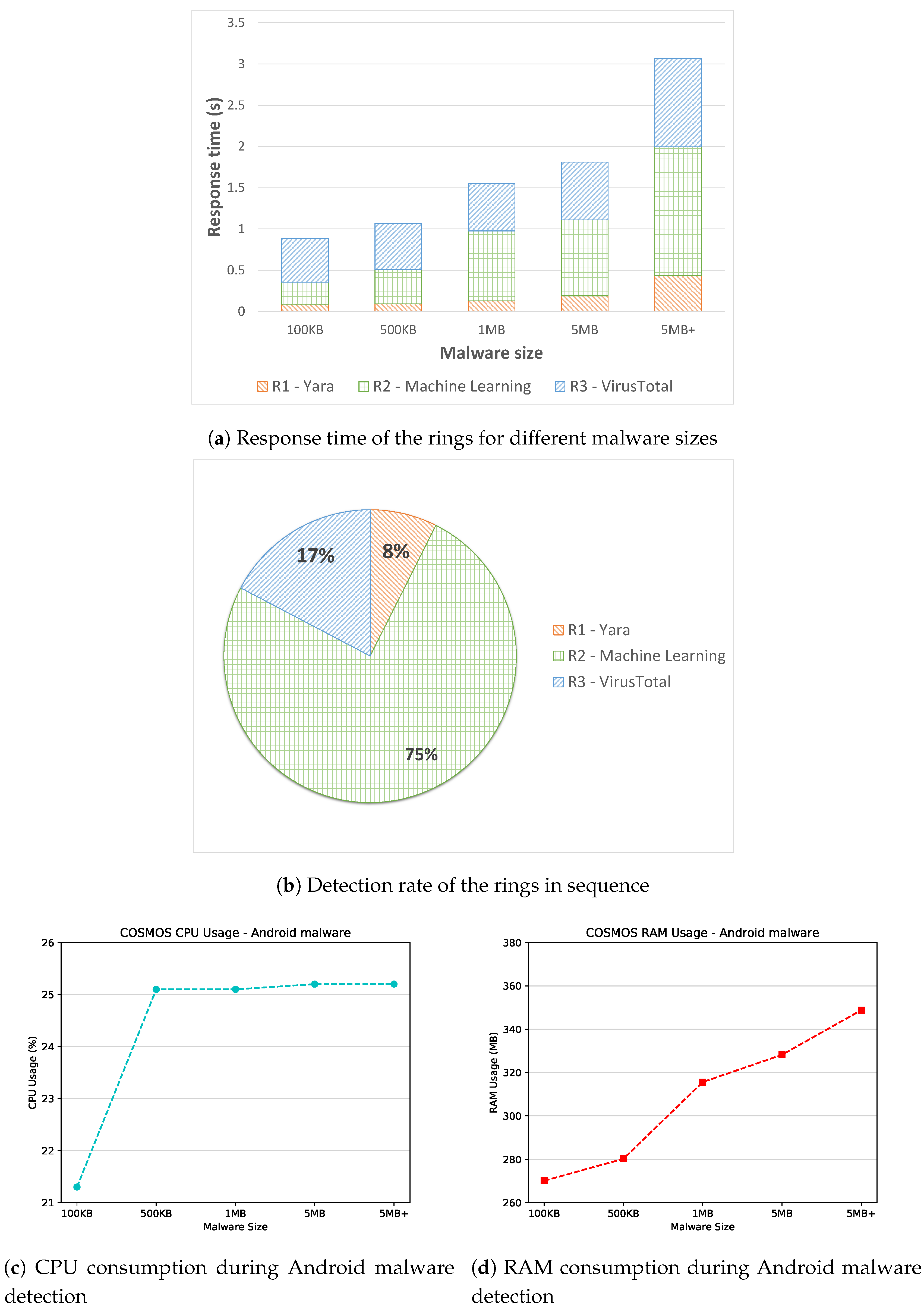
4.2.1. Android Malware Detection
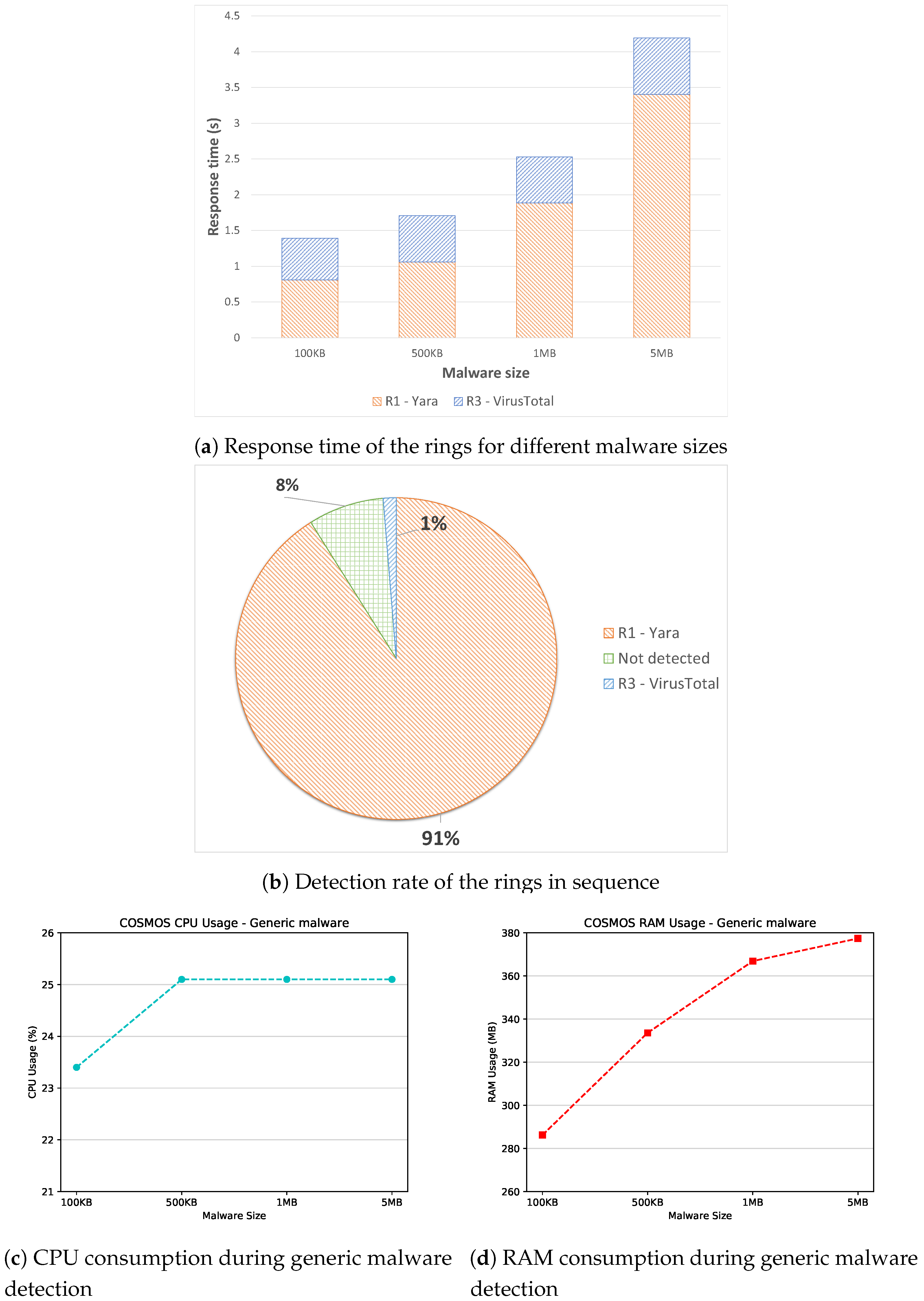
4.2.2. Non-Android Malware Detection
4.3. Challenges
5. COSMOS App
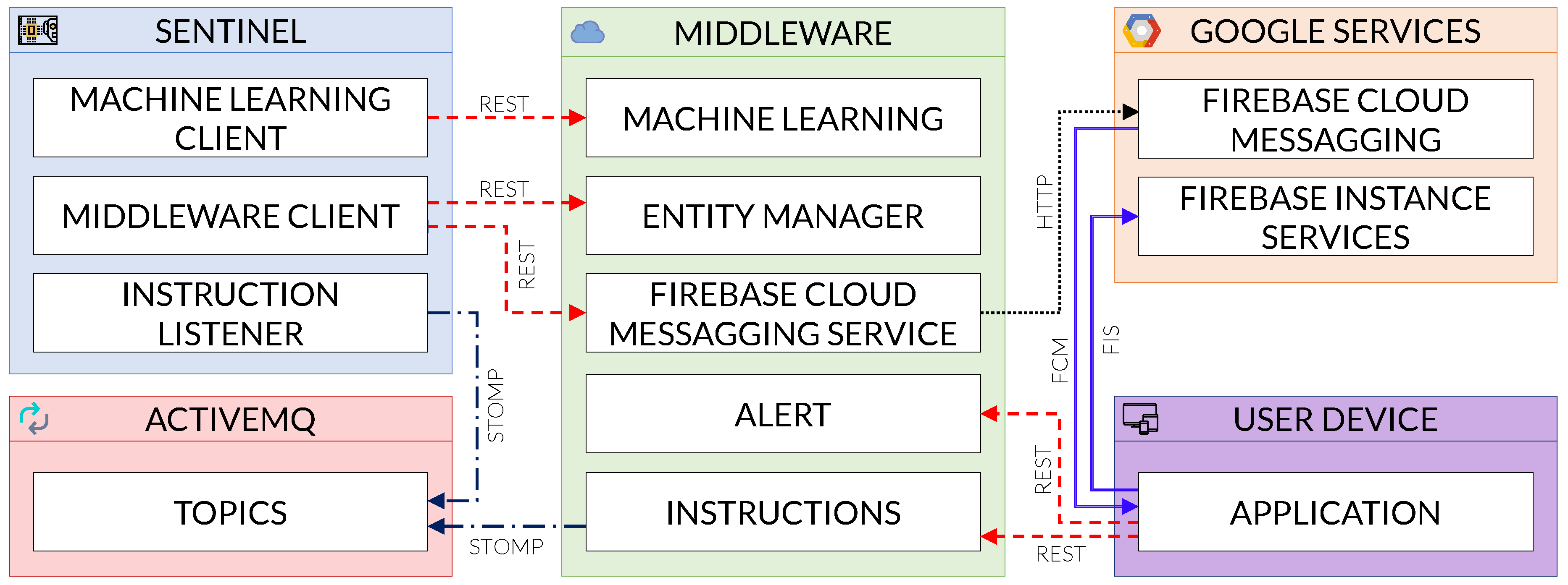
- Alert: This area manages all the App alerts, including alert information, statistics and persistence. This area does not receive information from the sentinel, as those alerts are taken by the Firebase Cloud Messaging Service for a better treatment.
- Entity Manager: This area manages all the entities in the middleware, providing CRUD operations for them. An entity is the representation of an actor in the COSMOS architecture, such as a Sentinel, the App, a Device or an Alert.
- Machine Learning (ML): This area manages the classification of samples into goodware or malware; it contains the ML model and, after receiving the characteristics, it returns the classification according to that model.
- Instructions: This area manages the exchange of instruction between the App and a selected sentinel, after receiving the instruction from the App, the middleware will publish it in the message broker, allowing for the called sentinel to read it and execute the instruction.
- Firebase Cloud Messaging (FCM) Service: This area receives the alert messages from the sentinel and forwards them to the App using the Google FCM API, the messages are received using the FCM instance manager, then a notification showing the message (and thus the alert) pops up.
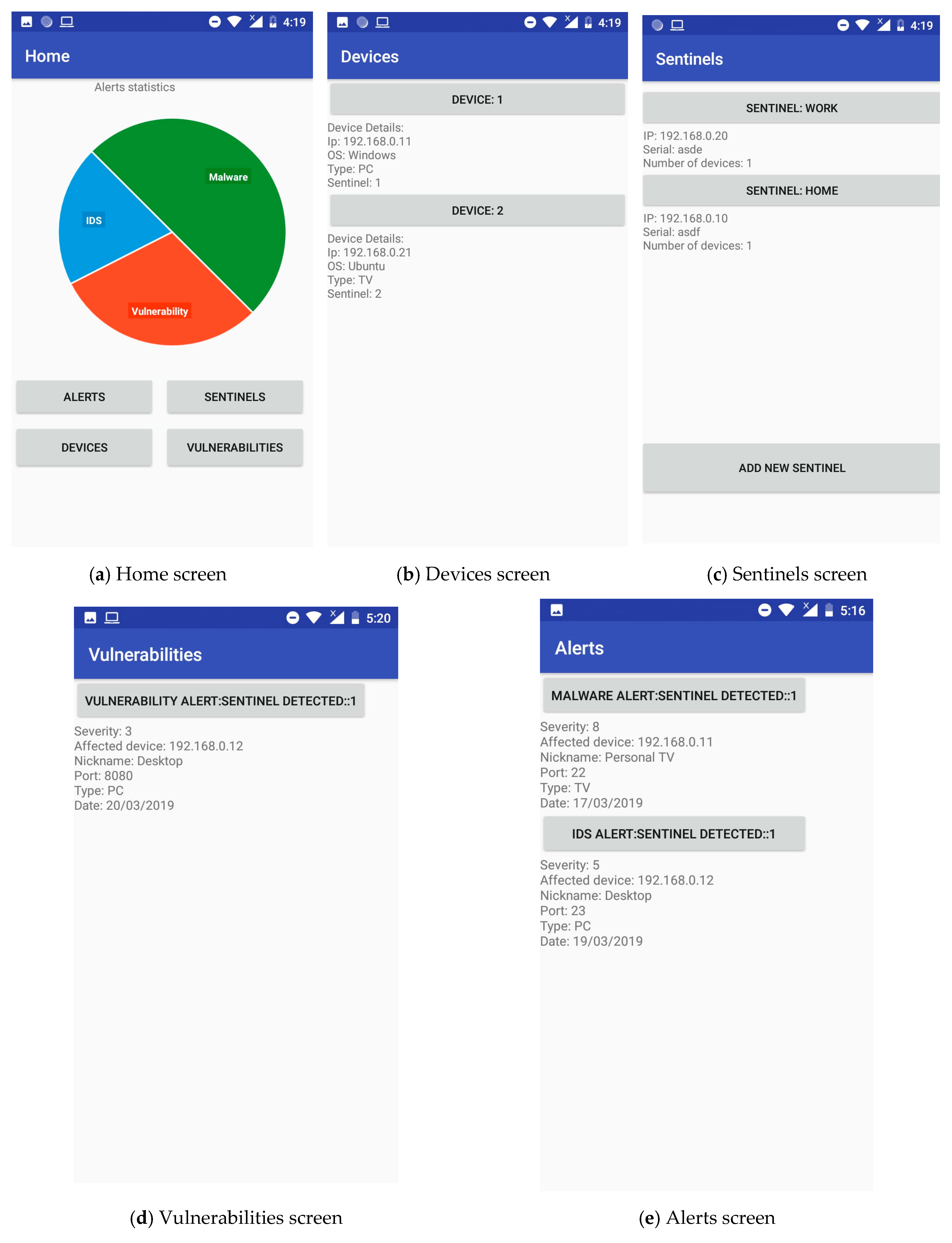
- Home: This screen is the entry point of the App and shows an overview of the alerts generated over the system(s) under protection of the sentinel(s) (Figure 8a).
- Devices: Through this screen, end-users can trigger a scanning of the environment of each of the registered sentinels in order to determine which devices should be protected (and which not). Moreover, some basic information is displayed for each signed-up device, such as operating system, IP address, vulnerabilities or pending alerts (Figure 8b).
- Sentinels: The binding process between sentinels and the App is performed here, allowing also to configure or even remove previously registered sentinels. Such process requires the association between the unique sentinel ID and the hash-generated App ID. As for the sentinels’ settings, things like stating a nickname (‘home’, ‘office’, etc.), for instance, are permitted (Figure 8c).
- Vulnerabilities: This screen provides a snapshot of the vulnerabilities found in each and every device selected to be protected by the sentinels. Some basic information regarding each vulnerability is shown, like the service or protocol affected, and the severity of the discovered vulnerability—for instance, (Figure 8d).
- Alerts: Last but not least, the Alerts screen gathers all the warnings submitted by the sentinels regarding intrusions and cyberattacks. For each of these alerts, further information such as the victim device, or even a number of potential countermeasures, is offered to the end-users (Figure 8e).
6. State of the Art
7. Conclusions and Future Work
Author Contributions
Acknowledgments
Conflicts of Interest
References
- Wang, T.; Zhang, G.; Liu, A.; Bhuiyan, M.Z.A.; Jin, Q. A Secure IoT Service Architecture with an Efficient Balance Dynamics Based on Cloud and Edge Computing. IEEE Internet Things J. 2018. [Google Scholar] [CrossRef]
- Yu, W.; Liang, F.; He, X.; Hatcher, W.G.; Lu, C.; Lin, J.; Yang, X. A Survey on the Edge Computing for the Internet of Things. IEEE Access 2018, 6, 6900–6919. [Google Scholar] [CrossRef]
- Nespoli, P.; Gómez Mármol, F. e-Health Wireless IDS with SIEM integration. In Proceedings of the IEEE Wireless Communications and Networking Conference (WCNC18), Barcelona, Spain, 15–18 April 2018. [Google Scholar]
- Díaz López, D.; Blanco Uribe, M.; Santiago Cely, C.; Tarquino Murgueitio, D.; Garcia Garcia, E.; Nespoli, P.; Gómez Mármol, F. Developing Secure IoT Services: A Security-Oriented Review of IoT Platforms. Symmetry 2018, 10, 669. [Google Scholar] [CrossRef]
- Gartner. Gartner’s 2016 Hype Cycle for Emerging Technologies Identifies Three Key Trends That Organizations Must Track to Gain Competitive Advantage. 2016. Available online: https://www.gartner.com/newsroom/id/3412017 (accessed on 11 August 2018).
- Charmonman, S.; Mongkhonvanit, P. Special consideration for Big Data in IoE or Internet of Everything. In Proceedings of the 13th International Conference on ICT and Knowledge Engineering (ICT Knowledge Engineering 2015), Bangkok, Thailand, 18–20 November 2015; pp. 147–150. [Google Scholar]
- Conti, M.; Dehghantanha, A.; Franke, K.; Watson, S. Internet of Things security and forensics: Challenges and opportunities. Future Gener. Comput. Syst. 2018, 78, 544–546. [Google Scholar] [CrossRef]
- Tweneboah-Koduah, S.; Skouby, K.E.; Tadayoni, R. Cyber Security Threats to IoT Applications and Service Domains. Wirel. Person. Commun. 2017, 95, 169–185. [Google Scholar] [CrossRef]
- Ling, Z.; Luo, J.; Xu, Y.; Gao, C.; Wu, K.; Fu, X. Security Vulnerabilities of Internet of Things: A Case Study of the Smart Plug System. IEEE Internet Things J. 2017, 4, 1899–1909. [Google Scholar] [CrossRef]
- Antonakakis, M.; April, T.; Bailey, M.; Bernhard, M.; Bursztein, E.; Cochran, J.; Durumeric, Z.; Halderman, J.A.; Invernizzi, L.; Kallitsis, M.; et al. Understanding the Mirai Botnet. In Proceedings of the 26th USENIX Conference on Security Symposium (SEC17), Vancouver, BC, Canada, 16–18 August 2017; pp. 1093–1110. [Google Scholar]
- Hwang, Y.H. IoT Security & Privacy: Threats and Challenges. In Proceedings of the 1st ACM Workshop on IoT Privacy, Trust, and Security (IoTPTS15), Singapore, 14 April 2015. [Google Scholar]
- Díaz López, D.; Blanco Uribe, M.; Santiago Cely, C.; Vega Torres, A.; Moreno Guataquira, N.; Morón Castro, S.; Nespoli, P.; Gómez Mármol, F. Shielding IoT against cyber-attacks: An event-based approach using SIEM. Wirel. Commun. Mob. Comput. 2018, 2018, 3029638. [Google Scholar] [CrossRef]
- Nespoli, P.; Zago, M.; Huertas Celdrán, A.; Gil Pérez, M.; Gómez Mármol, F.; García Clemente, F.J. A Dynamic Continuous Authentication Framework in IoT-Enabled Environments. In Proceedings of the Fifth International Conference on Internet of Things: Systems, Management and Security (IoTSMS 2018), Valencia, Spain, 15–18 October 2018; pp. 131–138. [Google Scholar]
- Lin, H.; Bergmann, N.W. IoT Privacy and Security Challenges for Smart Home Environments. Information 2016, 7, 44. [Google Scholar] [CrossRef]
- Kambourakis, G.; Gomez Marmol, F.; Wang, G. Security and Privacy in Wireless and Mobile Networks. Future Internet 2018, 10, 18. [Google Scholar] [CrossRef]
- Miettinen, M.; Marchal, S.; Hafeez, I.; Asokan, N.; Sadeghi, A.R.; Tarkoma, S. IoT SENTINEL: Automated Device-Type Identification for Security Enforcement in IoT. In Proceedings of the IEEE 37th International Conference on Distributed Computing Systems (ICDCS17), Atlanta, GA, USA, 5–8 June 2017; pp. 2177–2184. [Google Scholar]
- Ning, H.; Hong, L.; Yang, L.T. Cyberentity Security in the Internet of Things. Computer 2013, 46, 46–53. [Google Scholar] [CrossRef]
- Sforzin, A.; Gómez Mármol, F.; Conti, M.; Bohli, J.M. RPiDS: Raspberry Pi IDS A Fruitful Intrusion Detection System for IoT. In Proceedings of the IEEE Conference on Advanced and Trusted Computing, Toulouse, France, 18–21 July 2016; pp. 440–448. [Google Scholar]
- Vasilomanolakis, E.; Karuppayah, S.; Mühlhäuser, M.; Fischer, M. Taxonomy and Survey of Collaborative Intrusion Detection. ACM Comput. Surv. 2015, 47, 1–33. [Google Scholar] [CrossRef]
- Useche Peláez, D.; Díaz López, D.; Nespoli, P.; Gómez Mármol, F. TRIS: A Three-Rings IoT Sentinel to protect against cyber-threats. In Proceedings of the Fifth International Conference on Internet of Things: Systems, Management and Security (IoTSMS 2018), Valencia, Spain, 15–18 October 2018; pp. 123–130. [Google Scholar]
- Nespoli, P.; Papamartzivanos, D.; Mármol, F.G.; Kambourakis, G. Optimal Countermeasures Selection Against Cyber Attacks: A Comprehensive Survey on Reaction Frameworks. IEEE Commun. Surv. Tutor. 2018, 20, 1361–1396. [Google Scholar] [CrossRef]
- Papamartzivanos, D.; Gómez Mármol, F.; Kambourakis, G. Introducing Deep Learning Self-Adaptive Misuse Network Intrusion Detection Systems. IEEE Access 2019, 7, 13546–13560. [Google Scholar] [CrossRef]
- Snort. Network Intrusion Detection and Prevention System. Available online: https://www.snort.org/ (accessed on 26 March 2019).
- Pathan, A.S.K. The State of the Art in Intrusion Prevention and Detection; Taylor & Francis: Milton Park, Abingdon, UK, 2014. [Google Scholar]
- Kismet. Wireless Sniffer and Network Intrusion Detection System. Available online: https://www.kismetwireless.net (accessed on 26 March 2019).
- OpenVAS. Open Vulnerability Assessment System. Available online: http://www.openvas.org (accessed on 26 March 2019).
- Varsalone, J.; McFadden, M. Defense against the Black Arts: How Hackers Do What They Do and How to Protect against It; Taylor & Francis: Milton Park, Abingdon, UK, 2011. [Google Scholar]
- YARA. The Pattern Matching Swiss Knife for Malware Researchers. Available online: http://yara.readthedocs.io (accessed on 26 March 2019).
- Latifi, S. Information Technology: New Generations: 13th International Conference on Information Technology; Advances in Intelligent Systems and Computing; Springer International Publishing: Cham, Switzerland, 2016. [Google Scholar]
- Weka. Data Mining with Open Source Machine Learning Software. Available online: https://cs.waikato.ac.nz/ml/weka (accessed on 26 March 2019).
- Kaluža, B. Instant Weka How-to; Packt Publishing: Birmingham, UK, 2013. [Google Scholar]
- Koodous. Collaborative Platform for Android Malware Research. Available online: https://koodous.com (accessed on 26 March 2019).
- APKMirror. Free APK Downloads. Available online: https://www.apkmirror.com/ (accessed on 26 March 2019).
- Arp, D.; Spreitzenbarth, M.; Huebner, M.; Gascon, H.; Rieck, K. Drebin: Effective and Explainable Detection of Android Malware in Your Pocket. In Proceedings of the 21th Annual Network and Distributed System Security Symposium (NDSS14), San Diego, CA, USA, 23–26 February 2014; pp. 23–26. [Google Scholar]
- VirusTotal. Free On-Line File Analyzer. Available online: https://www.virustotal.com (accessed on 26 March 2019).
- Ciampa, M. CompTIA Security+ Guide to Network Security Fundamentals; Cengage Learning: Boston, MA, USA, 2017. [Google Scholar]
- Radare. Portable Reversing Framework. Available online: https://rada.re/r (accessed on 26 March 2019).
- Dunham, K.; Hartman, S.; Quintans, M.; Morales, J.A.; Strazzere, T. Android Malware and Analysis; Information Security Books; CRC Press: Boca Raton, FL, USA, 2014. [Google Scholar]
- Drake, J.J.; Lanier, Z.; Mulliner, C.; Fora, P.O.; Ridley, S.A.; Wicherski, G. Android Hacker’s Handbook; EBL-Schweitzer; Wiley: Hoboken, NJ, USA, 2014. [Google Scholar]
- OSSIM. Alienvault Open-Source SIEM. Available online: https://www.alienvault.com/products/ossim (accessed on 26 March 2019).
- Savas, O.; Deng, J. Big Data Analytics in Cybersecurity; Data Analytics Applications; CRC Press: Boca Raton, FL, USA, 2017. [Google Scholar]
- Akula, M.; Mahajan, A. Security Automation with Ansible 2: Leverage Ansible 2 to Automate Complex Security Tasks Like Application Security, Network Security, and Malware Analysis; Packt Publishing: Birmingham, UK, 2017. [Google Scholar]
- Dash, S.K.; Suarez-Tangil, G.; Khan, S.; Tam, K.; Ahmadi, M.; Kinder, J.; Cavallaro, L. DroidScribe: Classifying Android Malware Based on Runtime Behavior. In Proceedings of the IEEE Security and Privacy Workshops (SPW16), San Jose, CA, USA, 22–26 May 2016; pp. 252–261. [Google Scholar]
- Nespoli, P. WISS: Wireless IDS for IoT with SIEM integration. Master’s Thesis, University of Naples Federico II, Naples, Italy, 2017. [Google Scholar]
- Heriyanto, T.; Allen, L.; Ali, S. Kali Linux: Assuring Security by Penetration Testing; Packt Publishing: Birmingham, UK, 2014. [Google Scholar]
- Aho, A.V.; Corasick, M.J. Efficient String Matching: An Aid to Bibliographic Search. Commun. ACM 1975, 18, 333–340. [Google Scholar] [CrossRef]
- Yara Rules. Yara Rules Official Repository. Available online: https://github.com/Yara-Rules (accessed on 26 March 2019).
- Ronen, R.; Radu, M.; Feuerstein, C.; Yom-Tov, E.; Ahmadi, M. Microsoft Malware Classification Challenge. arXiv, 2018; arXiv:1802.10135. [Google Scholar]
- Offensive Computing. Free Malware Download. Available online: http://www.offensivecomputing.net/ (accessed on 26 March 2019).
- Virus Sign. Malware Research and Data Center. Available online: http://www.virussign.com/ (accessed on 26 March 2019).
- Zelter. Malware Sample Sources. Available online: https://zeltser.com/malware-sample-sources/ (accessed on 26 March 2019).
- Ning, H.; Liu, H. Cyber-Physical-Social Based Security Architecture for Future Internet of Things. Adv. Internet Things 2012, 2, 1–7. [Google Scholar] [CrossRef]
- Dorri, A.; Kanhere, S.; Jurdak, R. Blockchain in internet of things: Challenges and Solutions. arXiv, 2016; arXiv:1608.05187. [Google Scholar]
- Tor Project. Anonymity online. Available online: https://www.torproject.org/ (accessed on 26 March 2019).
- Riahi, A.; Challal, Y.; Natalizio, E.; Chtourou, Z.; Bouabdallah, A. A Systemic Approach for IoT Security. In Proceedings of the IEEE International Conference on Distributed Computing in Sensor Systems, Cambridge, MA, USA, 21–23 May 2013; pp. 351–355. [Google Scholar]
- Babar, S.; Stango, A.; Prasad, N.; Sen, J.; Prasad, R. Proposed embedded security framework for Internet of Things (IoT). In Proceedings of the 2nd IEEE International Conference on Wireless Communication, Vehicular Technology, Information Theory and Aerospace & Electronic Systems Technology (Wireless VITAE), Chennai, India, 28 February–3 March 2011; pp. 1–5. [Google Scholar]
- Rahman, A.F.A.; Daud, M.; Mohamad, M.Z. Securing Sensor to Cloud Ecosystem using Internet of Things (IoT) Security Framework. In Proceedings of the International Conference on Internet of things and Cloud Computing—ICC ’16, Cambridge, UK, 22–23 March 2016; pp. 1–5. [Google Scholar]
- Abie, H.; Balasingham, I. Risk-based Adaptive Security for Smart IoT in eHealth. In Proceedings of the 7th International Conference on Body Area Networks (BodyNets12), Oslo, Norway, 24–26 September 2012; pp. 269–275. [Google Scholar]
- Cheng, S.M.; Chen, P.Y.; Lin, C.C.; Hsiao, H.C. Traffic-Aware Patching for Cyber Security in Mobile IoT. IEEE Commun. Mag. 2017, 55, 29–35. [Google Scholar] [CrossRef]
- Roux, J.; Alata, E.; Auriol, G.; Nicomette, V.; Kaâniche, M. Toward an Intrusion Detection Approach for IoT based on Radio Communications Profiling. In Proceedings of the 13th European Dependable Computing Conference, Geneva, Switzerland, 4–8 September 2017; pp. 147–150. [Google Scholar]
- Hodo, E.; Bellekens, X.; Hamilton, A.; Dubouilh, P.L.; Iorkyase, E.; Tachtatzis, C.; Atkinson, R. Threat analysis of IoT networks using artificial neural network intrusion detection system. In Proceedings of the 2016 International Symposium on Networks, Computers and Communications (ISNCC16), Hammamet, Tunisia, 11–13 May 2016; pp. 1–6. [Google Scholar]
- Meidan, Y.; Bohadana, M.; Shabtai, A.; Ochoa, M.; Tippenhauer, N.O.; Guarnizo, J.D.; Elovici, Y. Detection of Unauthorized IoT Devices Using Machine Learning Techniques. arXiv, 2017; arXiv:1709.04647. [Google Scholar]
- Hasan, M.A.M.; Nasser, M.; Ahmad, S.; Molla, K.I. Feature selection for intrusion detection using random forest. J. Inf. Secur. 2016, 7, 129. [Google Scholar] [CrossRef]
- Pa, Y.M.P.; Suzuki, S.; Yoshioka, K.; Matsumoto, T.; Kasama, T.; Rossow, C. IoTPOT: A Novel Honeypot for Revealing Current IoT Threats. J. Inf. Process. 2016, 24, 522–533. [Google Scholar] [CrossRef]
- Sivaraman, V.; Gharakheili, H.H.; Vishwanath, A.; Boreli, R.; Mehani, O. Network-level security and privacy control for smart-home IoT devices. In Proceedings of the IEEE 11th International Conference on Wireless and Mobile Computing, Networking and Communications (WiMob15), Abu Dhabi, UAE, 19–21 October 2015; pp. 163–167. [Google Scholar]


| Category | Name | Description |
|---|---|---|
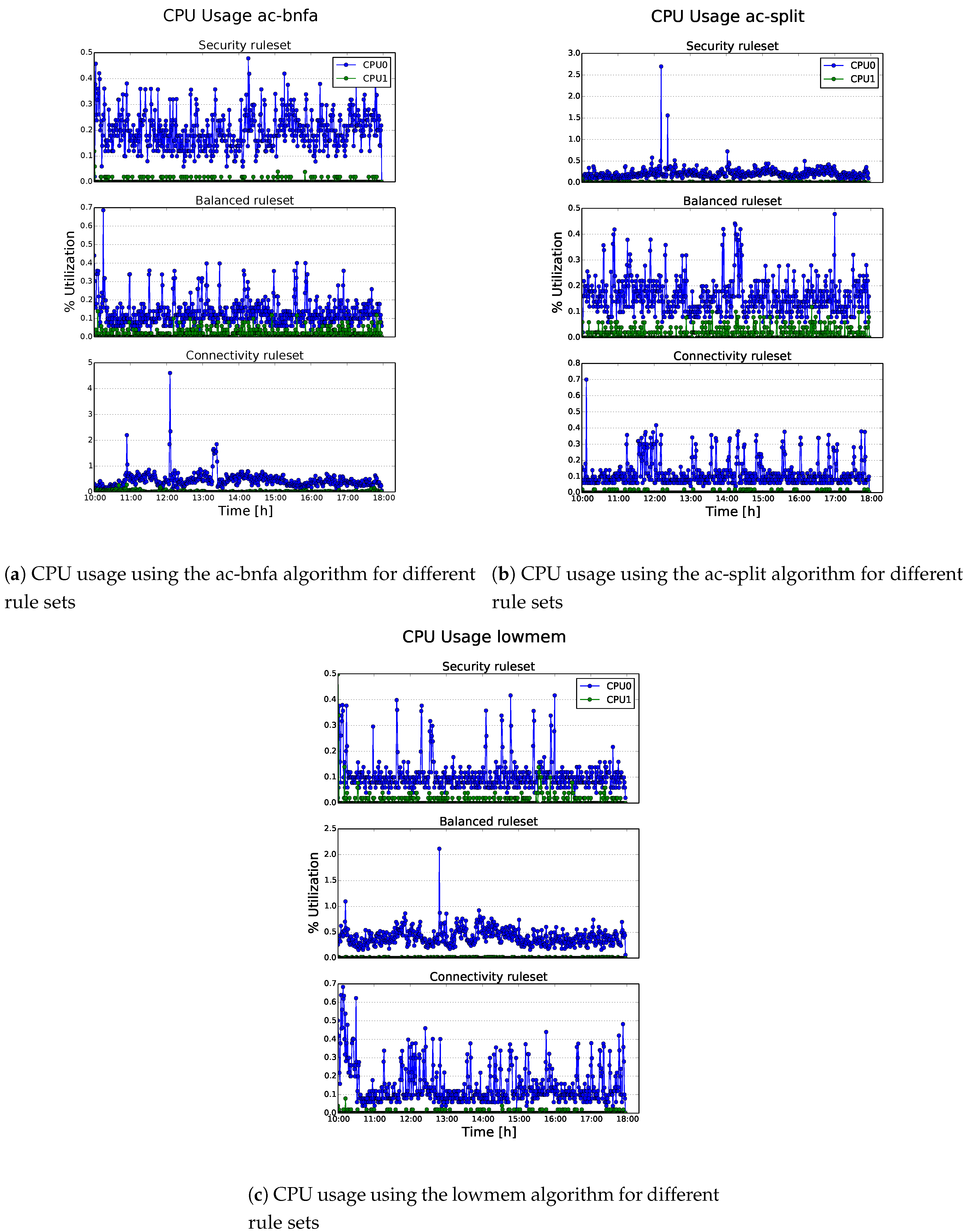
| Statistics | CPU | Raspberry Pi CPU usage along an experiment time lapse |
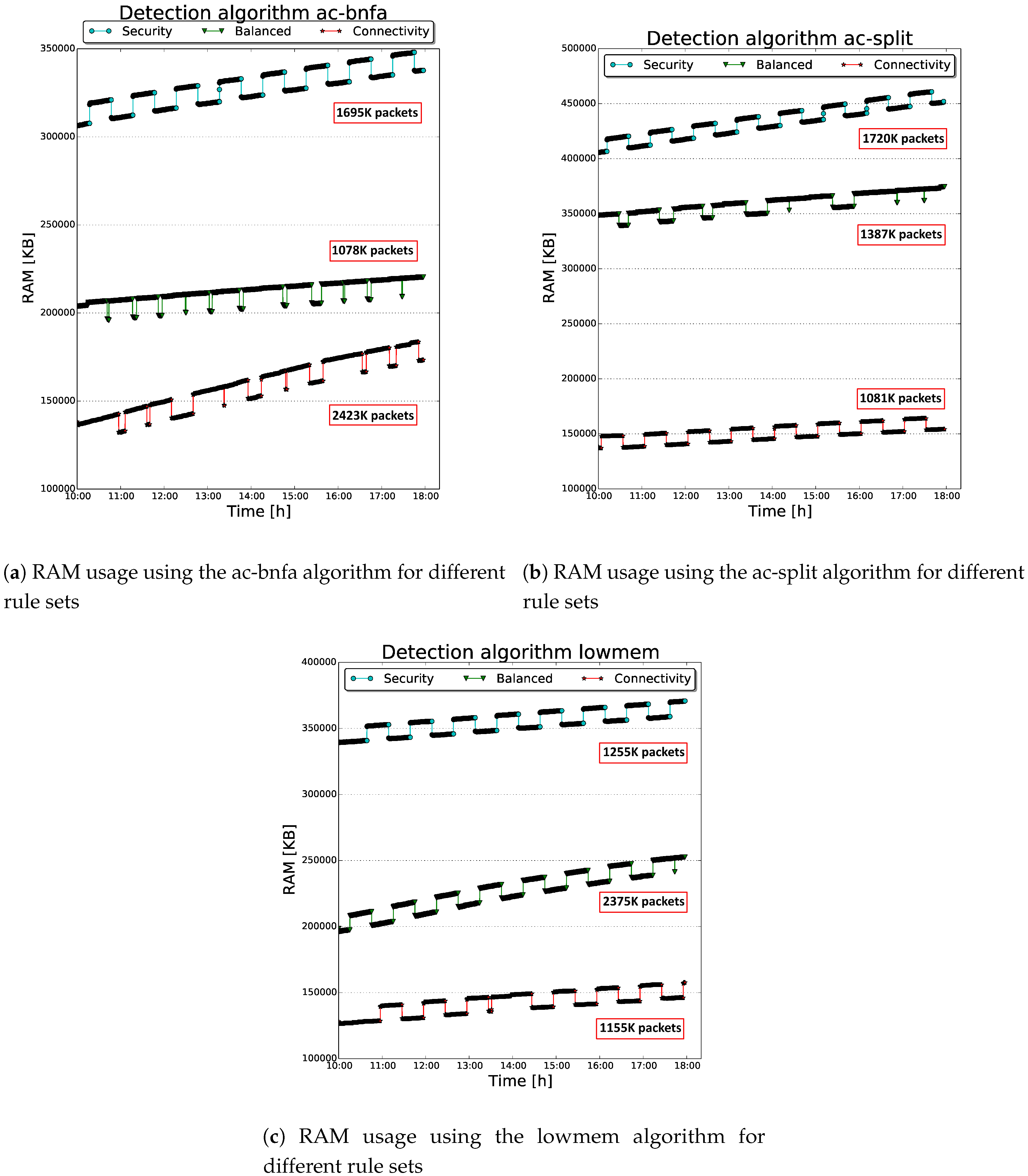
| RAM | Raspberry Pi RAM usage along an experiment time lapse | |
| Analyzed packets | No. of packets analyzed from the IDSs | |
| Input | RuleSets | {connectivity, balanced, security} |
| Detection Algorithms | {lowmem, ac-bnfa, ac-split} | |
| Time window | 8-h |
| Name | Description |
|---|---|
| CPU | Raspberry Pi CPU usage for a given experiment |
| RAM | Raspberry Pi RAM usage for a given experiment |
| Response time | Time required to analyze a sample |
| Detection rate | Percentage of detected malware |
| Related Work | Methodology | Scenario | Security Goals | |||
|---|---|---|---|---|---|---|
| SG1 | SG2 | SG3 | SG4 | |||
| Ning and Liu [52] | Security from three perspectives | IoT ecosystem | N.A. | ✗ | ✓ | N.A. |
| Dorri et al. [53] | Adapt current technology to IoT Scenario | Smart Home | ✓ | N.A. | ✗ | ✓ |
| Riahi et al. [55] | Systematic approach to improve IoT security | IoT ecosystem | N.A. | N.A. | N.A. | N.A. |
| Babar et al. [56] | Embedded security in all stages of device lifecycle | IoT ecosystem | ✓ | ✗ | ✗ | ✓ |
| Rahman et al. [57] | Embedded security in each layer of the IoT ecosystem | IoT ecosystem | ✓ | ✗ | ✓ | ✓ |
| Abie and Balasingham [58] | Risk management based security | e-Health | N.A. | ✗ | ✓ | N.A. |
| Cheng et al. [59] | Traffic aware patching intermediate nodes | IoT ecosystem | ✓ | ✗ | ✗ | N.A. |
| Roux et al. [60] | Identification of suspicious behavior at physical layer | IoT network | ✓ | ✗ | ✗ | ✗ |
| Hodo et al. [61] | Detection of DDoS attacks | IoT network | ✓ | ✗ | ✓ | ✗ |
| Meidan et al. [62] | Detection of unauthorized devices in the network | IoT network | ✓ | ✗ | ✓ | ✗ |
| Pa et al. [64] | Honeypot and Sandboxing | IoT ecosystem | ✗ | ✗ | ✗ | ✓ |
| Sivaraman et al. [65] | SDN Networks to detect and block devices | IoT network | ✓ | ✗ | ✗ | ✗ |
| Sforzin et al. [18] | Single-board computer IDS | Smart Home | ✓ | ✗ | ✗ | ✓ |
| Nespoli and Gómez Mármol [3] | Wireless IDS with SIEM integration | e-Health | ✓ | ✗ | ✓ | ✓ |
| Miettinen et al. [16] | IoT Sentinel to protect and identify IoT nodes | IoT network | ✓ | ✗ | ✗ | ✗ |
© 2019 by the authors. Licensee MDPI, Basel, Switzerland. This article is an open access article distributed under the terms and conditions of the Creative Commons Attribution (CC BY) license (http://creativecommons.org/licenses/by/4.0/).
Share and Cite
Nespoli, P.; Useche Pelaez, D.; Díaz López, D.; Gómez Mármol, F. COSMOS: Collaborative, Seamless and Adaptive Sentinel for the Internet of Things. Sensors 2019, 19, 1492. https://doi.org/10.3390/s19071492
Nespoli P, Useche Pelaez D, Díaz López D, Gómez Mármol F. COSMOS: Collaborative, Seamless and Adaptive Sentinel for the Internet of Things. Sensors. 2019; 19(7):1492. https://doi.org/10.3390/s19071492
Chicago/Turabian StyleNespoli, Pantaleone, David Useche Pelaez, Daniel Díaz López, and Félix Gómez Mármol. 2019. "COSMOS: Collaborative, Seamless and Adaptive Sentinel for the Internet of Things" Sensors 19, no. 7: 1492. https://doi.org/10.3390/s19071492
APA StyleNespoli, P., Useche Pelaez, D., Díaz López, D., & Gómez Mármol, F. (2019). COSMOS: Collaborative, Seamless and Adaptive Sentinel for the Internet of Things. Sensors, 19(7), 1492. https://doi.org/10.3390/s19071492