A Simple Procedure to Assess Limit of Detection for Multisensor Systems

 , , and
Abstract
:1. Introduction
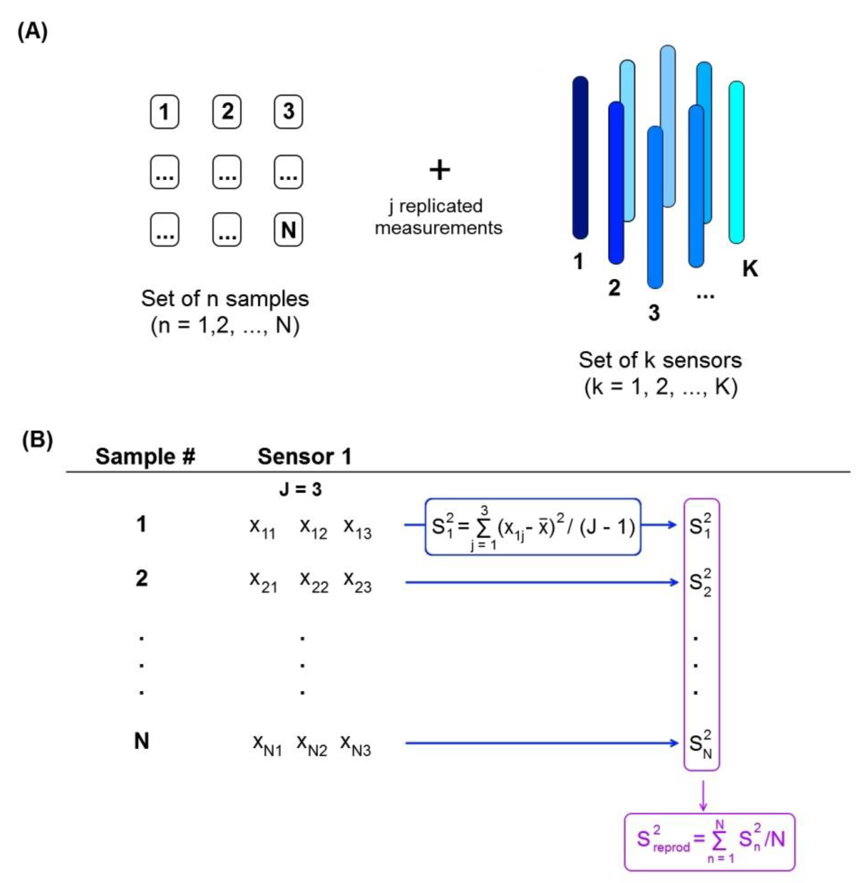
2. Theory
2.1. LOD Interval Calculation
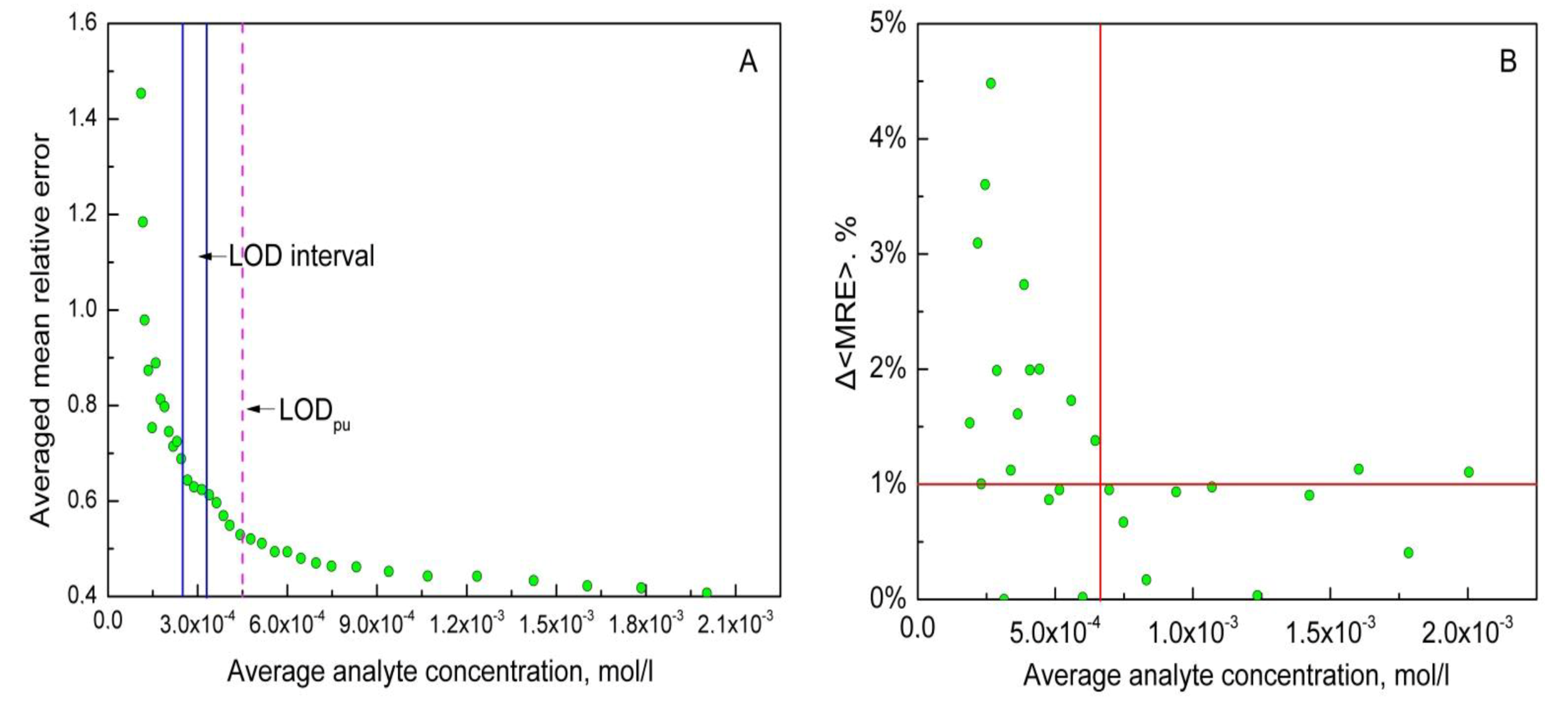
2.2. Mean Relative Error Evolution Approach
- sort the column with measured analyte concentration yn in ascending order (yn becomes );
- calculate MRE for each sample;
- average MRE values and the measured concentrations for the first n samples (with the lowest concentration). n = 2 is the most convenient choice. Than use step by step the following formula:
- calculate the increment of averaged MRE as Δ<MRE> = |MREn+1′ − MREn′|.
3. Experimental
3.1. Multisensor Systems
3.2. Data Processing
4. Results and Discussion
4.1. Multisensor System for Ca2+ Quantification in Ca/Mg/Na Mixture
4.2. Multisensor System for La Quantification in La/Y/Gd Mixtures
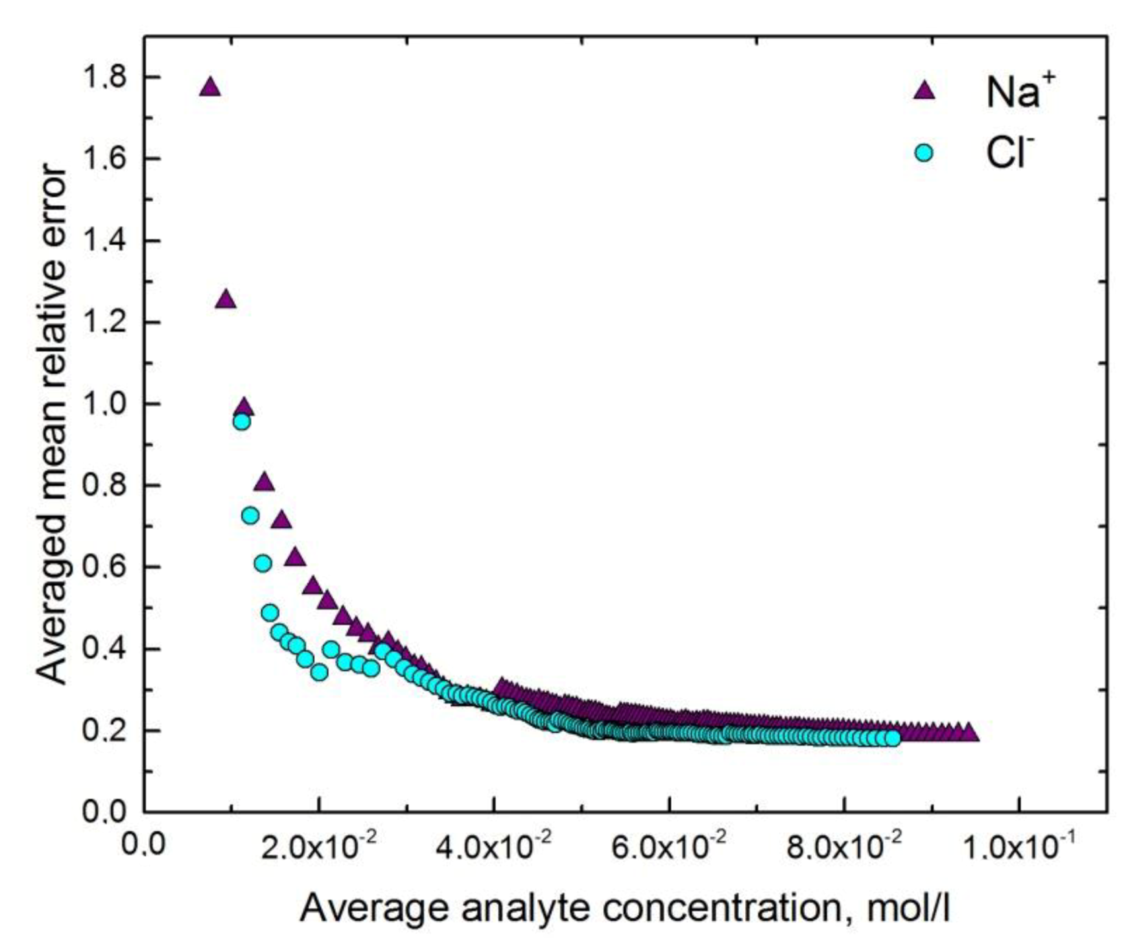
4.3. Multisensor System for Determination of Urine Ionic Composition
5. Conclusions
- the PLS model (or any other regression model) has to be optimized;
- sample concentration values should uniformly cover the concentration range.
Supplementary Materials
Author Contributions
Funding
Conflicts of Interest
References
- Vlasov, Y.; Legin, A.; Rudnitskaya, A.; di Natale, C.; D’Amico, A. Nonspecific sensor arrays (“electronic tongue”) for chemical analysis of liquids (IUPAC Technical Report). Pure Appl. Chem. 2005, 77, 1965–1983. [Google Scholar] [CrossRef]
- Riul, A., Jr.; Dantas, C.; Miyazaki, C.; Oliveira, O., Jr. Recent advances in electronic tongues. Analyst 2010, 135, 2481–2495. [Google Scholar] [CrossRef]
- Del Valle, M. Electronic tongues employing electrochemical sensors. Electroanalysis 2010, 22, 1539–1555. [Google Scholar] [CrossRef]
- Kirsanov, D.; Zadorozhnaya, O.; Krasheninnikov, A.; Komarova, N.; Popov, A.; Legin, A. Water toxicity evaluation in terms of bioassay with an Electronic Tongue. Sens. Actuators B 2013, 179, 282–286. [Google Scholar] [CrossRef]
- Smyth, H.; Cozzolino, D. Instrumental methods (spectroscopy, electronic nose, and tongue) as tools to predict taste and aroma in beverages: Advantages and limitations. Chem. Rev. 2013, 113, 1429–1440. [Google Scholar] [CrossRef] [PubMed]
- Li, Z.; Suslick, K. A hand-held optoelectronic nose for the identification of liquors. ACS Sens. 2018, 3, 121–127. [Google Scholar] [CrossRef] [PubMed]
- LaGasse, M.; McCormick, K.; Khanjian, H.; Schilling, M.; Suslick, K. Colorimetric sensor arrays: Development and application to art conservation. J. Am. Inst. Conserv. 2018, 57, 127–140. [Google Scholar] [CrossRef]
- Olivieri, A. Practical guidelines for reporting results in single- and multi-component analytical calibration: A tutorial. Anal. Chem. Acta 2015, 868, 10–22. [Google Scholar] [CrossRef]
- Vlasov, Y. Problems of Analytical Chemistry; Nauka: Moscow, Russia, 2011. [Google Scholar]
- Buck, R.P.; Lindner, E. Recommendations for nomenclature of ionselective electrodes. Pure Appl. Chem. 1994, 66, 2527–2536. [Google Scholar] [CrossRef]
- Bakker, E.; Pretsch, E. Potentiometric sensors for trace-level analysis. Trends Anal. Chem. 2005, 24, 199–207. [Google Scholar] [CrossRef]
- Faber, K.; Kowalski, B. Propagation of measurement errors for the validation of predictions obtained by principal component regression and partial least squares. J. Chemometr. 1997, 11, 181–238. [Google Scholar] [CrossRef]
- Ortiz, M.; Sarabia, L.; Herrero, A.; Sánchez, M.; Sanz, M.; Rueda, M.; Giménez, D.; Meléndez, M. Capability of detection of an analytical method evaluating false positive and false negative (ISO 11843) with partial least squares. Chemom. Intell. Lab. Syst. 2003, 69, 21–33. [Google Scholar] [CrossRef]
- Delaney, M. Multivariate detection limits for selected ion monitoring gas chromatography-mass spectrometry. Chemom. Intell. Lab. Syst. 1988, 3, 45–51. [Google Scholar] [CrossRef]
- Boqué, R.; Larrechi, M.; Rius, F. Multivariate detection limits with fixed probabilities of error. Chemom. Intell. Lab. Syst. 1999, 45, 397–408. [Google Scholar] [CrossRef]
- Faber, N.; Bro, R. Standard error of prediction for multiway PLS: 1. Background and a simulation study. Chemom. Intell. Lab. Syst. 2002, 61, 133–149. [Google Scholar] [CrossRef]
- Lorber, A.; Faber, K.; Kowalski, B. Net Analyte Signal Calculation in Multivariate Calibration. Anal. Chem. 1997, 69, 1620–1626. [Google Scholar] [CrossRef]
- Burgués, J.; Jiménez-Soto, J.; Marco, S. Using Net Analyte Signal to Estimate the Limit of Detection in Temperature-modulated MOX Sensors. Procedia Eng. 2016, 168, 436–439. [Google Scholar] [CrossRef]
- Allegrini, F.; Olivieri, A. IUPAC-Consistent Approach to the Limit of Detection in Partial Least-Squares Calibration. Anal. Chem. 2014, 86, 7858–7866. [Google Scholar] [CrossRef]
- Olivieri, A. Analytical Figures of Merit: From Univariate to Multiway Calibration. Chem. Rev. 2014, 114, 5358–5378. [Google Scholar] [CrossRef]
- Olivieri, A. A simple approach to uncertainty propagation in preprocessed multivariate calibration. J. Chemom. 2002, 16, 207–217. [Google Scholar] [CrossRef]
- Allegrini, F.; Wentzell, P.; Olivieri, A. Generalized error-dependent prediction uncertainty in multivariate calibration. Anal. Chim. Acta 2016, 903, 51–60. [Google Scholar] [CrossRef]
- Olivieri, A.; Faber, N.; Ferré, J.; Boqué, R.; Kalivas, J.; Mark, H. Uncertainty estimation and figures of merit for multivariate calibration (IUPAC Technical Report). Pure Appl. Chem. 2006, 78, 633–661. [Google Scholar] [CrossRef]
- Burgués, J.; Santiago, M. Multivariate estimation of the limit of detection by orthogonal partial least squares in temperature-modulated MOX sensors. Anal. Chim. Acta 2018, 1019, 49–64. [Google Scholar] [CrossRef]
- Cochran, W. The distribution of the largest of a set of estimated variances as a fraction of their total. Ann. Hum. Genet. 1941, 11, 47–52. [Google Scholar] [CrossRef]
- ISO Standard 5725–2:1994: Accuracy (Trueness and Precision) of Measurement Methods and Results—Part 2: Basic Method for the Determination of Repeatability and Reproducibility of a Standard Measurement Method; International Organization for Standardization: Geneva, Switzerland, 1994.
- UE’t Lam, R. Scrutiny of variance results for outliers: Cochran’s test optimized. Anal. Chim. Acta 2012, 659, 68–84. [Google Scholar] [CrossRef]
- Kirsanov, D.; Khaydukova, M.; Tkachenko, L.; Legin, A.; Babain, V. Potentiometric Sensor Array for Analysis of Complex Rare Earth Mixtures. Electroanalysis 2012, 24, 121–130. [Google Scholar] [CrossRef]
- Yaroshenko, I.; Kirsanov, D.; Kartsova, L.; Sidorova, A.; Borisova, I.; Legin, A. Determination of urine ionic composition with potentiometric multisensor system. Talanta 2015, 131, 556–561. [Google Scholar] [CrossRef]
- Wold, S.; Sjöström, M.; Eriksson, L. PLS-regression: A basic tool of chemometrics. Chemom. Intell. Lab. Syst. 2001, 58, 109–130. [Google Scholar] [CrossRef]


| Multisensor System | Composition of the Solution under Study | Analyte | Concentration Range, mmol/L | Number of Sensors |
|---|---|---|---|---|
| 1 | Ca/Mg + Na (background) | Ca2+ | 0.1–9.9 | 10 |
| 2 | La/Y/Gd | La3+ | 0.01–1 | 24 |
| 3 | Urine | Na+ | 3.8–255.5 | 22 |
| Cl− | 11.1–22.3 |
| Analyte | PLS Model Characteristics | LOD Calculation, mol/L | ||||
|---|---|---|---|---|---|---|
| Slope | R2 | RMSECV | LODmin | LODmax | LODpu | |
| Ca2+ | 0.90 | 0.89 | 7.27 × 10⁻⁴ | 2.5 × 10⁻⁴ | 3.3 × 10⁻⁴ | 4.5 × 10⁻⁴ |
| Object of Analysis | Analyte | PLS Model Characteristics | LOD Calculation | ||
|---|---|---|---|---|---|
| Slope | R2 | RMSECV | LODpu, mol/L | ||
| La/Y/Gd | La3+ | 0.92 | 0.91 | 9.02 × 10⁻⁵ | 4.4 × 10⁻⁴ |
| Urine | Na+ | 0.83 | 0.83 | 2.17 × 10⁻² | 8.0 × 10⁻² |
| Cl− | 0.83 | 0.83 | 1.93 × 10⁻² | 6.2 × 10⁻² | |
| Analyte | LODpu, mol/L | Estimated LOD, mol/L |
|---|---|---|
| Ca2+ | 4.5 × 10⁻⁴ | 6 × 10⁻⁴ |
| La3+ | 4.4 × 10⁻⁴ | 3 × 10⁻⁴ |
| Na+ | 8.0 × 10⁻² | 4 × 10⁻² |
| Cl− | 6.2 × 10⁻² | 3 × 10⁻² |
© 2019 by the authors. Licensee MDPI, Basel, Switzerland. This article is an open access article distributed under the terms and conditions of the Creative Commons Attribution (CC BY) license (http://creativecommons.org/licenses/by/4.0/).
Share and Cite
Oleneva, E.; Khaydukova, M.; Ashina, J.; Yaroshenko, I.; Jahatspanian, I.; Legin, A.; Kirsanov, D. A Simple Procedure to Assess Limit of Detection for Multisensor Systems. Sensors 2019, 19, 1359. https://doi.org/10.3390/s19061359
Oleneva E, Khaydukova M, Ashina J, Yaroshenko I, Jahatspanian I, Legin A, Kirsanov D. A Simple Procedure to Assess Limit of Detection for Multisensor Systems. Sensors. 2019; 19(6):1359. https://doi.org/10.3390/s19061359
Chicago/Turabian StyleOleneva, Ekaterina, Maria Khaydukova, Julia Ashina, Irina Yaroshenko, Igor Jahatspanian, Andrey Legin, and Dmitry Kirsanov. 2019. "A Simple Procedure to Assess Limit of Detection for Multisensor Systems" Sensors 19, no. 6: 1359. https://doi.org/10.3390/s19061359
APA StyleOleneva, E., Khaydukova, M., Ashina, J., Yaroshenko, I., Jahatspanian, I., Legin, A., & Kirsanov, D. (2019). A Simple Procedure to Assess Limit of Detection for Multisensor Systems. Sensors, 19(6), 1359. https://doi.org/10.3390/s19061359