A Novel Calibration Method of Articulated Laser Sensor for Trans-Scale 3D Measurement


Abstract
1. Introduction
2. Principle of Articulated Laser Sensor
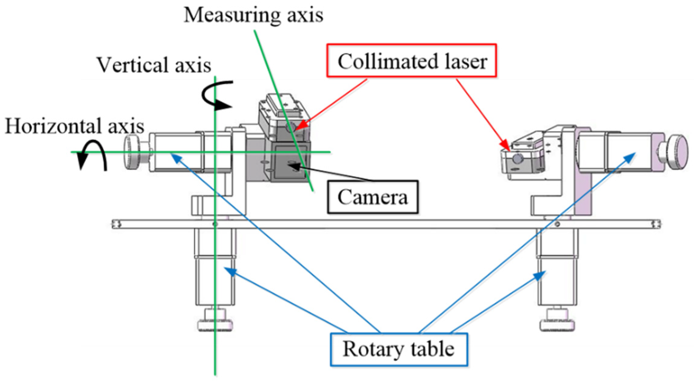
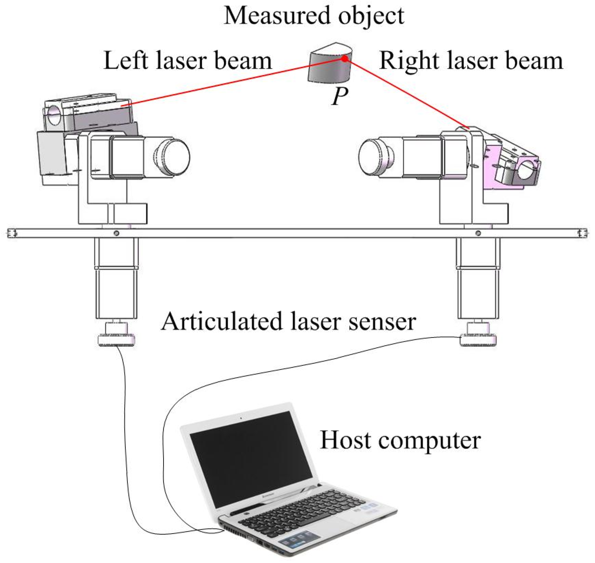
2.1. System Construction
2.2. Measurement Principle
3. Calibration Principle
3.1. Calibration of the Vertical and Horizontal Axes
- (1)
- Based on least squares methods, a plane is fitted utilizing the centers of the porcelain beads, which are measured by CMM.
- (2)
- The distances from the measured points to the fitted plane are calculated. If the distance is more than the threshold, these points are eliminated and another plane is fitted again.
- (3)
- The normal vector of fitted plane is recorded as the direction vector of the rotation axis.
- (4)
- The remaining points are projected onto the fitted plane.
- (5)
- Based on least squares methods, an ellipse is fitted utilizing the projected points.
- (6)
- The center of fitted ellipse is recorded as the fixed point of rotation axis.
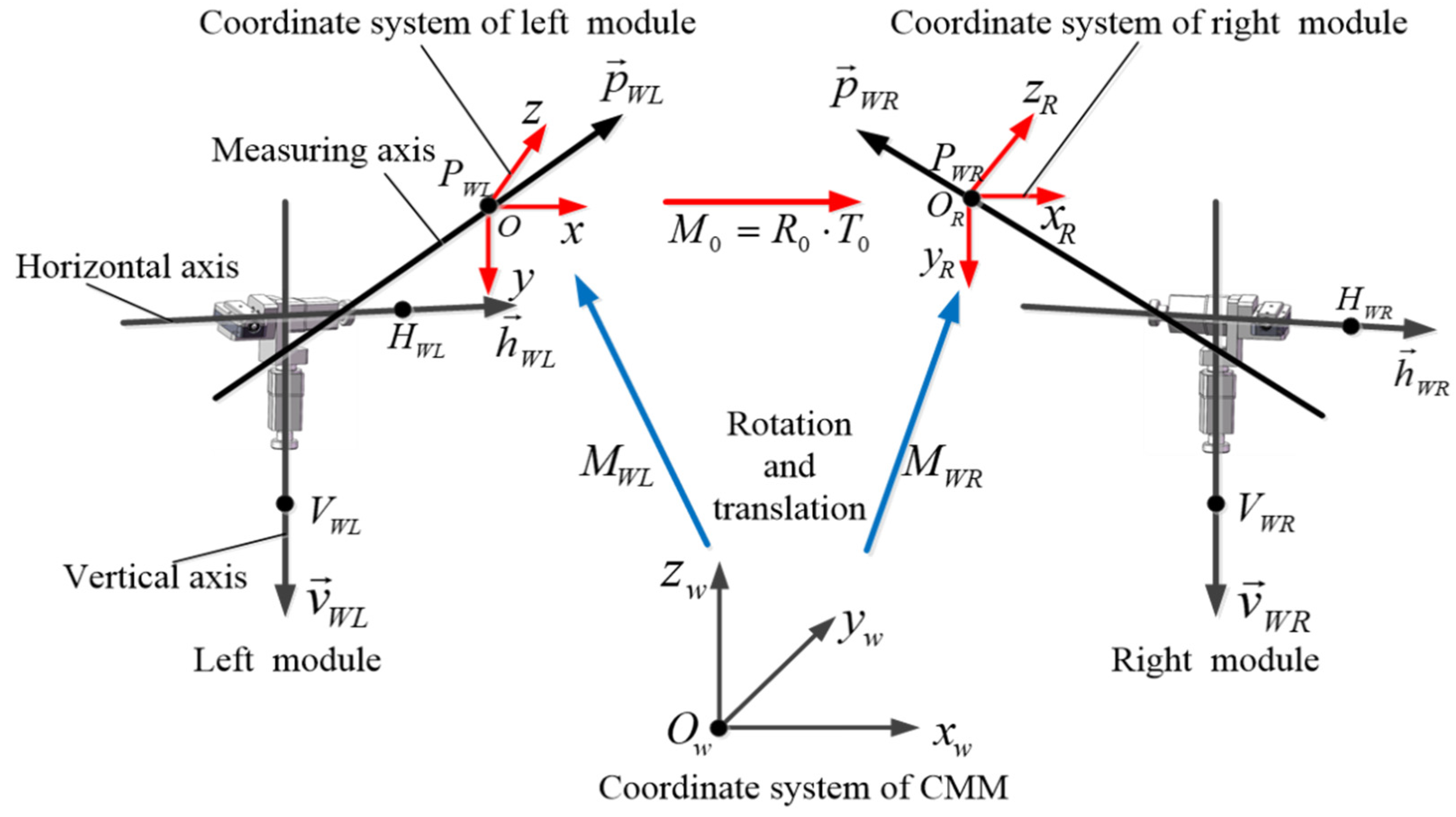
3.2. Calibration of the Laser Beam
- (1)
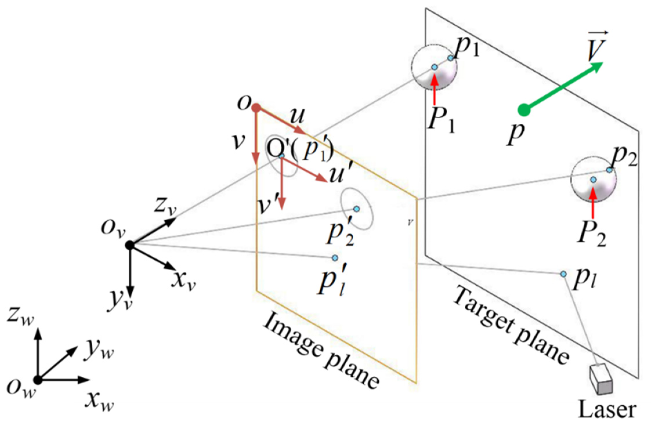
- The world coordinate system is defined as . The CMM’s measurement coordinate system is regarded as world coordinate system.
- (2)
- The viewpoint coordinate system is defined as . The axis is perpendicular to the target plane, and the and coordinates of origin are equal to the and coordinates of .
- (3)
- The actual coordinate system of pixels on CCD is defined as .
- (4)
- The image plane coordinate system is defined as . The axis is parallel to axis, and the and coordinates of origin are equal to the and coordinates of .
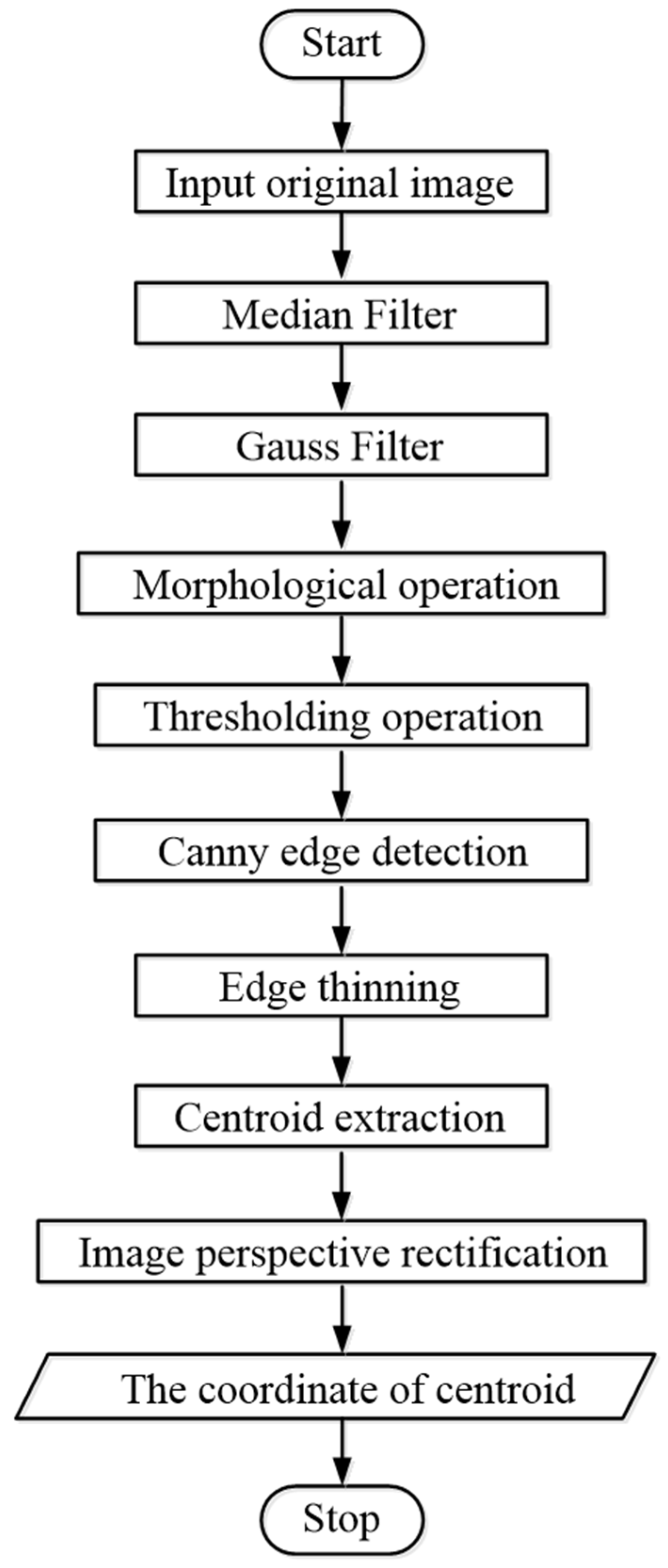
4. Image Processing
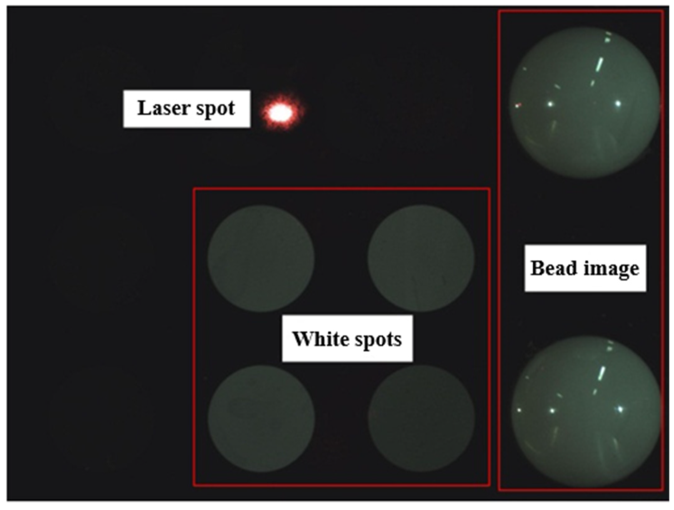
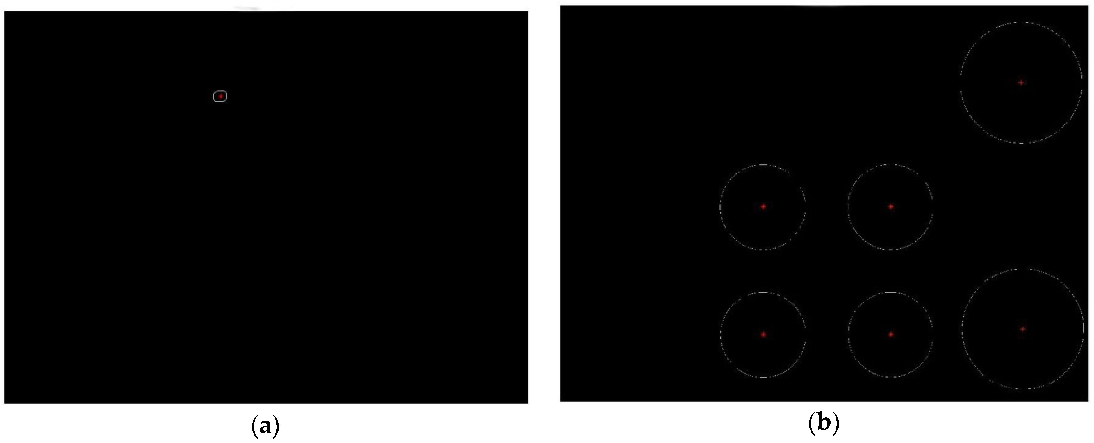
4.1. Centroid Extraction
4.2. Image Perspective Rectification
- (1)
- The image is rotated to ensure that is parallel to the axis. According to the coordinates , , and after rotation, the vanishing point coordinate is obtained.
- (2)
- The expression of the rectification in u-axis direction is
- (3)
- where is the width of square,
- (4)
- and the expression of the rectification in the axis direction is
- (5)
- After the rectification in the axis and the axis direction, is parallel to , but is not parallel to . The image is rotated 90°, and the rectification in the axis and the axis direction is executed again.
5. Experiment
5.1. Calibration of the Vertical and Horizontal Axes
5.2. Calibration of the Laser Beam
- (1)
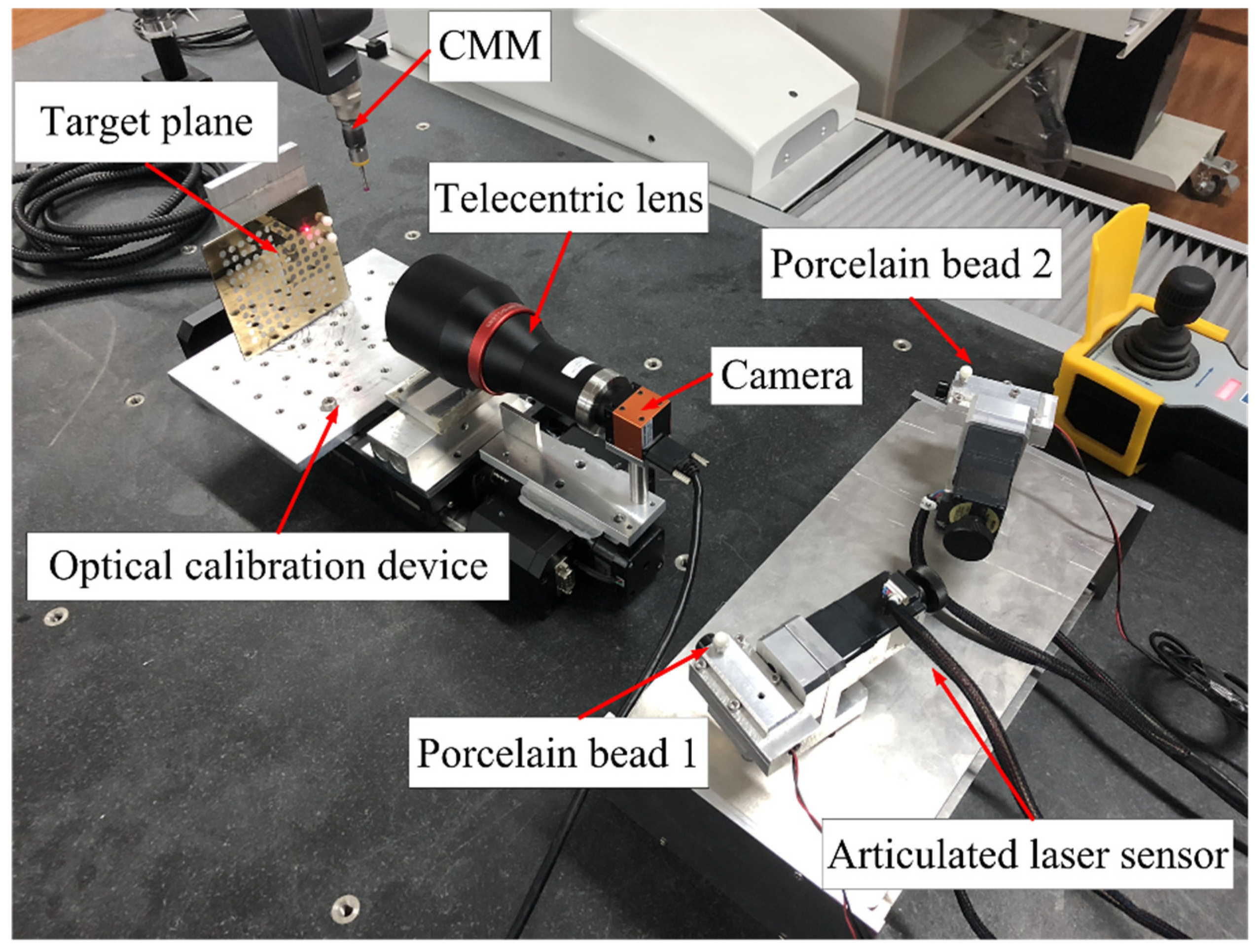
- The articulated laser sensor is fixed on the operating platform of CMM.
- (2)
- The optical calibration device is adjusted to ensure that the laser beam can project onto the target plane.
- (3)
- The centers of two beads are measured by CMM, and the coordinates are recorded as and , respectively.
- (4)
- Nine points on the target plane are measured by CMM and used to fit a plane. The parameters of the target plane are obtained, including the unit normal vector recorded as and a point on the plane recorded as .
- (5)
- An image is collected by a camera with telecentric lens.
- (6)
- Steps (2)–(5) are repeated more than seven times.
- (7)
- The collected images are processed as described in the Section 4.
- (8)
- Based on the least square method, a spatial line is fitted from the coordinates of the laser spots in the CMM’s coordinate system.
- (9)
- The parameters of the laser beam are obtained, including the direction vector and a fixed point on the laser beam, as shown in Table 4.
5.3. Calibration of Extrinsic Parameters
5.4. Verification Experiment
6. Conclusions
Author Contributions
Funding
Conflicts of Interest
References
- Lee, R.T.; Shiou, F.J. Multi-beam laser probe for measuring position and orientation of freeform surface. Measurement 2011, 44, 1–10. [Google Scholar] [CrossRef]
- Sun, X.; Zhang, Q. Dynamic 3-D shape measurement method: A review. Opt. Lasers Eng. 2010, 48, 191–204. [Google Scholar]
- Zhang, Q.; Sun, X.; Xiang, L.; Sun, X. 3-D shape measurement based on complementary Gray-code light. Opt. Lasers Eng. 2012, 50, 574–579. [Google Scholar] [CrossRef]
- Feng, D.; Feng, M.; Ozer, E.; Fukuda, Y. A Vision-Based Sensor for Noncontact Structural Displacement Measurement. Sensors 2015, 15, 16557–16575. [Google Scholar] [CrossRef] [PubMed]
- Muralikrishnan, B.; Phillips, S.; Sawyer, D. Laser trackers for large-scale dimensional metrology: A review. Precis. Eng. 2016, 44, 13–28. [Google Scholar] [CrossRef]
- Ouyang, J.F.; Liu, W.L.; Yan, Y.G.; Sun, D.X. Angular error calibration of laser tracker system. SPIE 2006, 6344, 6344–6348. [Google Scholar]
- Scherer, M.; Lerma, J. From the conventional total station to the prospective image assisted photogrammetric scanning total station: Comprehensive review. J. Surv. Eng. 2009, 135, 173–178. [Google Scholar] [CrossRef]
- Wu, B.; Wang, B. Automatic Measurement in Large-Scale Space with the Laser Theodolite and Vision Guiding Technology. Adv. Mech. Eng. 2013, 5, 1–8. [Google Scholar] [CrossRef]
- Zhou, F.; Peng, B.; Cui, Y.; Wang, Y.; Tan, H. A novel laser vision sensor for omnidirectional 3D measurement. Opt. Laser Technol. 2013, 45, 1–12. [Google Scholar] [CrossRef]
- Wu, B.; Yang, F.; Ding, W.; Xue, T. A novel calibration method for non-orthogonal shaft laser theodolite measurement system. Rev. Sci. Instrum. 2016, 87, 035102. [Google Scholar] [CrossRef] [PubMed]
- Bi, C.; Liu, Y.; Fang, J.-G.; Guo, X.; Lv, L.-P.; Dong, P. Calibration of laser beam direction for optical coordinate measuring system. Measurement 2015, 73, 191–199. [Google Scholar]
- Sun, J.; Zhang, J.; Liu, Z.; Zhang, G. A vision measurement model of laser displacement sensor and its calibration method. Opt. Lasers Eng. 2013, 51, 1344–1352. [Google Scholar] [CrossRef]
- Xie, Z.; Wang, J.; Zhang, Q. Complete 3D measurement in reverse engineering using a multi-probe system. Mach. Tools Manuf. 2005, 45, 1474–1486. [Google Scholar]
- Yang, T.; Wang, Z.; Wu, Z.; Li, X.; Wang, L.; Liu, C. Calibration of Laser Beam Direction for Inner Diameter Measuring Device. Sensors 2017, 17, 294. [Google Scholar] [CrossRef] [PubMed]
- Xie, Z.; Wang, X.; Chi, S. Simultaneous calibration of the intrinsic and extrinsic parameters of structured-light sensors. Opt. Lasers Eng. 2014, 58, 9–18. [Google Scholar] [CrossRef]
- Yang, K.; Yu, H.-Y.; Yang, C. Calibration of line structured-light vision measurement system based on free-target. J. Mech. Electr. Eng. 2016, 33, 1066–1070. [Google Scholar]
- Smith, K.B.; Zheng, Y.F. Point laser triangulation probe calibration for coordinate metrology. J. Manuf. Sci. Eng. 2000, 122, 582–593. [Google Scholar] [CrossRef]
- Wu, D.; Chen, T.; Li, A. A High Precision Approach to Calibrate a Structured Light Vision Sensor in a Robot-Based Three-Dimensional Measurement System. Sensors 2016, 16, 1388. [Google Scholar] [CrossRef] [PubMed]
- Yin, S.; Ren, Y.; Guo, Y.; Zhu, J.; Yang, S.; Ye, S. Development and calibration of an integrated 3D scanning system for high-accuracy large-scale metrology. Measurement 2014, 54, 65–76. [Google Scholar] [CrossRef]
- Men, Y.; Zhang, G.; Men, C.; Li, X.; Ma, N. A Stereo Matching Algorithm Based on Four-Moded Census and Relative Confidence Plane Fitting. Chin. J. Electron. 2015, 24, 807–812. [Google Scholar] [CrossRef]
- Mulleti, S.; Seelamantula, C.S. Ellipse Fitting Using the Finite Rate of Innovation Sampling Principle. IEEE Trans. Image Process. 2016, 25, 1451–1464. [Google Scholar] [CrossRef] [PubMed]
- Yang, J.; Zhang, T.; Song, J.; Liang, B. High accuracy error compensation algorithm for star image sub-pixel subdivision location. Opt. Lasers Eng. 2010, 18, 1002–1010. [Google Scholar]
- Luo, X.; Du, Z. Method of Image Perspective Transform Based on Double Vanishing Point. Comput. Eng. 2009, 35, 212–214. [Google Scholar]
- Gu, F.; Zhao, H. Analysis and correction of projection error of camera calibration ball. Acta Opt. Sin. 2012, 12, 209–215. [Google Scholar]


| Category | Parameters | Physical Meaning | |
|---|---|---|---|
| Intrinsic parameters | Vertical axis | Vector | Direction of vertical axis |
| Point | Fixed point of vertical axis | ||
| Horizontal axis | Vector | Direction of horizontal axis | |
| Point | Fixed point of horizontal axis | ||
| Measuring axis | Vector | Direction of measuring axis | |
| Point | Fixed point of measuring axis | ||
| Extrinsic parameters | Rotation–translation matrix | Rotation matrix | Rotation from to |
| Translation vector | Translation from to | ||
| Point | ||||
|---|---|---|---|---|
| Category | Intrinsic Parameters | |
|---|---|---|
| Left module | Horizontal axis | Fixed point (160.919,162.305,−622.648) Direction vector (0.954,−0.300,0.005) |
| Vertical axis | Fixed point (208.213,147.371,−604.198) Direction vector (0.006,−0.002,−0.999) | |
| Right module | Horizontal axis | Fixed point (416.534,157.549,−622.284) Direction vector (0.973,0.232,−0.004) |
| Vertical axis | Fixed point (368.818,146.245,−603.301) Direction vector (−0.002,−0.003,−0.999) | |
| Category | Intrinsic Parameters | |
|---|---|---|
| Left module | Measuring axis | Fixed point (313.363,702.058,−618.860) |
| Direction vector (0.270,0.963,0.005) | ||
| Right module | Measuring axis | Fixed point (252.987,691.699,−619.093) |
| Direction vector (−0.2934,0.956,0.003) | ||
| Point No. | Left/Right Module | Horizontal Angle (°) | Vertical Angle (°) | Measured Length (mm) | Real Length (mm) | Deviation (mm) |
|---|---|---|---|---|---|---|
| 1 | Left | 0.000 | 0.000 | 91.747 | 91.752 | −0.005 |
| Right | −15.775 | −0.108 | ||||
| 2 | Left | 14.986 | −0.057 | |||
| Right | −0.052 | 0.012 | ||||
| 3 | Left | 33.143 | −1.342 | 166.854 | 164.831 | 0.023 |
| Right | 38.992 | −1.258 | ||||
| 4 | Left | 15.786 | −1.325 | |||
| Right | 17.184 | −1.277 | ||||
| 5 | Left | 12.152 | −1.475 | 172.134 | 172.141 | −0.007 |
| Right | 12.206 | −1.447 | ||||
| 6 | Left | 9.647 | 19.920 | |||
| Right | 3.046 | 20.580 | ||||
| 7 | Left | −8.503 | 20.021 | 157.470 | 157.467 | 0.003 |
| Right | −12.452 | 18.288 | ||||
| 8 | Left | −31.538 | 19.282 | |||
| Right | −29.141 | 15.717 | ||||
| 9 | Left | −0.848 | 14.621 | 128.730 | 128.753 | −0.023 |
| Right | 4.000 | 14.582 | ||||
| 10 | Left | 11.500 | 13.578 | |||
| Right | 17.800 | 14.570 | ||||
| 11 | Left | 12.500 | −1.744 | 352.831 | 352.781 | 0.050 |
| Right | −1.102 | −1.754 | ||||
| 12 | Left | 26.000 | 12.595 | |||
| Right | 35.000 | 14.606 |
© 2019 by the authors. Licensee MDPI, Basel, Switzerland. This article is an open access article distributed under the terms and conditions of the Creative Commons Attribution (CC BY) license (http://creativecommons.org/licenses/by/4.0/).
Share and Cite
Kang, J.; Wu, B.; Duan, X.; Xue, T. A Novel Calibration Method of Articulated Laser Sensor for Trans-Scale 3D Measurement. Sensors 2019, 19, 1083. https://doi.org/10.3390/s19051083
Kang J, Wu B, Duan X, Xue T. A Novel Calibration Method of Articulated Laser Sensor for Trans-Scale 3D Measurement. Sensors. 2019; 19(5):1083. https://doi.org/10.3390/s19051083
Chicago/Turabian StyleKang, Jiehu, Bin Wu, Xiaodeng Duan, and Ting Xue. 2019. "A Novel Calibration Method of Articulated Laser Sensor for Trans-Scale 3D Measurement" Sensors 19, no. 5: 1083. https://doi.org/10.3390/s19051083
APA StyleKang, J., Wu, B., Duan, X., & Xue, T. (2019). A Novel Calibration Method of Articulated Laser Sensor for Trans-Scale 3D Measurement. Sensors, 19(5), 1083. https://doi.org/10.3390/s19051083