Figure 1.
Number of visible satellites from different systems with an elevation mask of 10 degrees (top) and from all the four systems with different elevation masks (bottom). The figures were generated based on the MGEX combined broadcast ephemeris on DOY 224, 2018 for station CUAA located in Perth, Australia. G, E, J and I are denoted as system identifications for GPS, Galileo, QZSS and IRNSS, respectively.
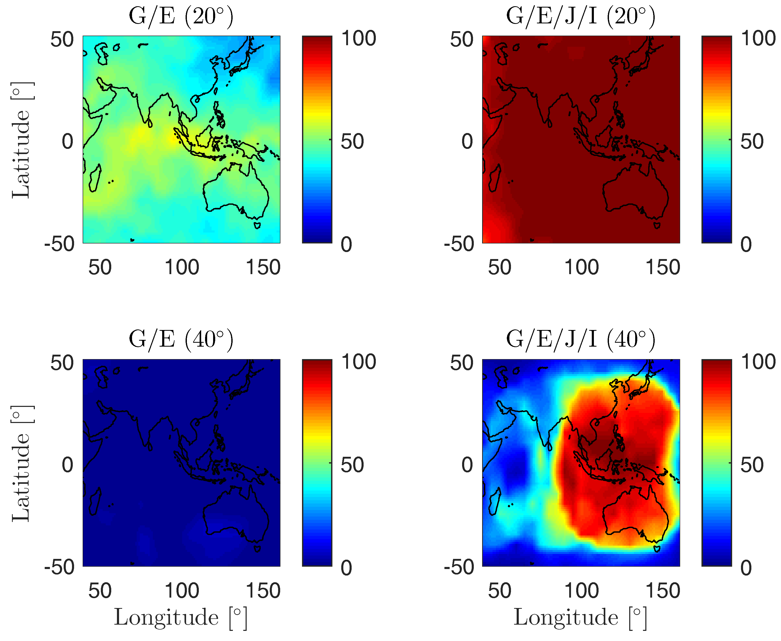
Figure 2.
Percentages with the 24 h period that at least eight satellites are above the elevation mask of 20 (top) and 40 degrees (bottom). The figure was generated based on the MGEX combined broadcast ephemeris on DOY 224, 2018 with a data sampling interval of 30 s. The newly launched I09 and the QZSS satellite J07 were not contained in the broadcast ephemeris. The satellite positions (WGS84) of J07 on DOY 154, 2018 were used for the computation.
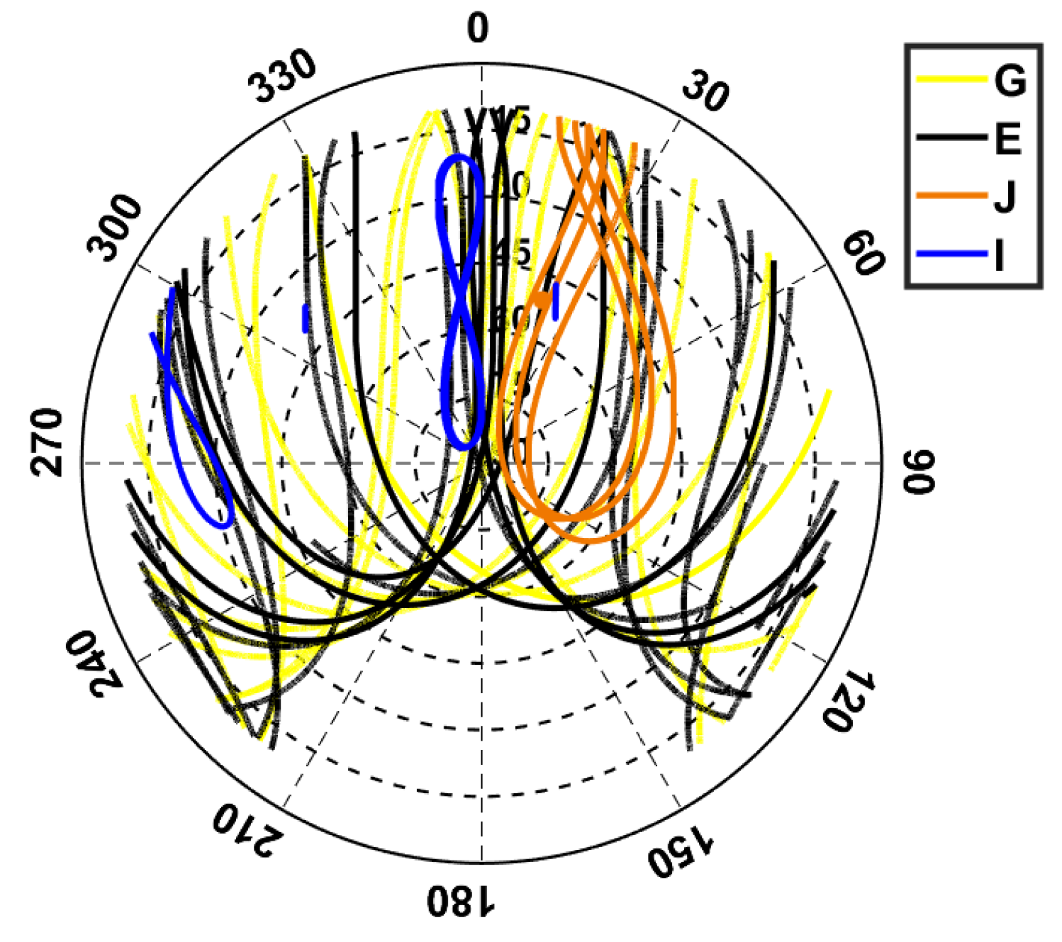
Figure 3.
Skyplot for station CUAA on DOY 224, 2018. An elevation mask of 10 degrees was set for the plot.
Figure 3.
Skyplot for station CUAA on DOY 224, 2018. An elevation mask of 10 degrees was set for the plot.
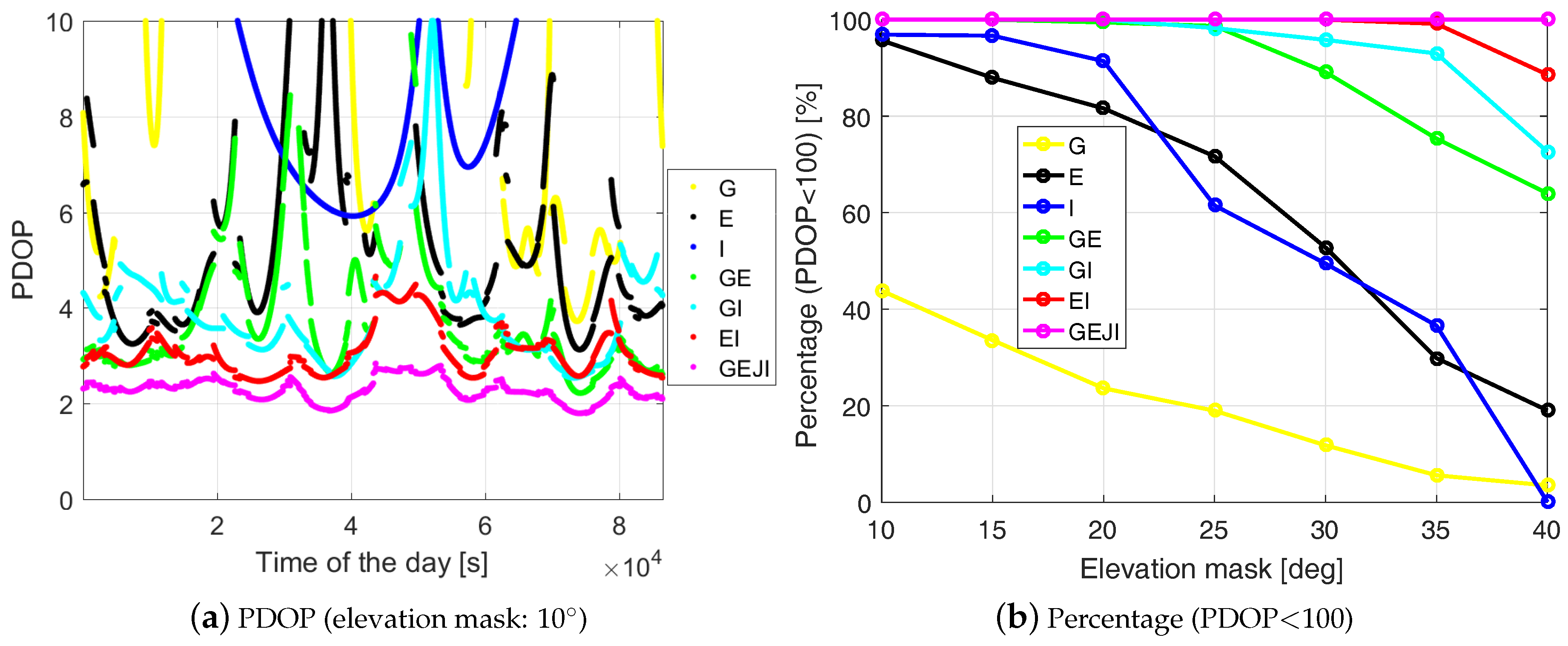
Figure 4.
PDOP (Equation (
6)) with an elevation mask of 10 degrees (
a) and the percentages within a 24 h period that PDOP is smaller than 100 (
b). The ground truth of baseline CUAA-CUCC and the satellite geometry on DOY 224, 2018 were used for the plots. Satellite positions (WGS84) of J07 on DOY 154, 2018 were used for the plots. The data sampling rate is 1 Hz. Note that (
a) is zoomed out to 0–10.
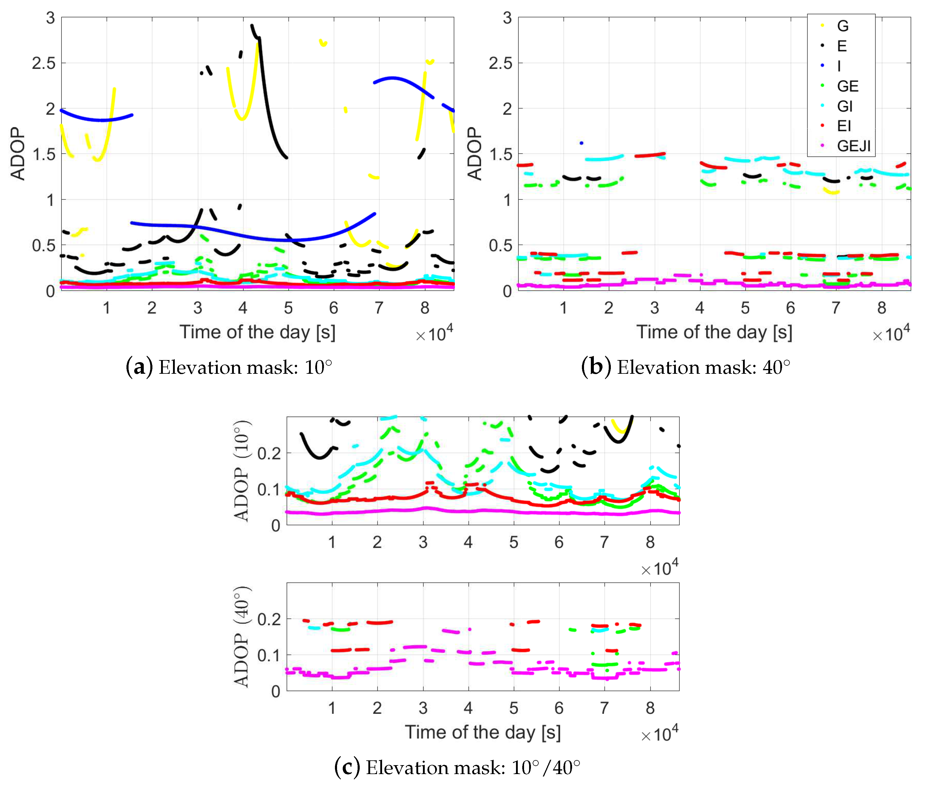
Figure 5.
ADOP (Equation (
10)) of baseline CUAA-CUCC on DOY 224, 2018 with elevation masks of 10 (
a); 40 degrees (
b) and the figures zoomed out for small ADOP values (
c). The data sampling rate is 1 Hz.
Figure 5.
ADOP (Equation (
10)) of baseline CUAA-CUCC on DOY 224, 2018 with elevation masks of 10 (
a); 40 degrees (
b) and the figures zoomed out for small ADOP values (
c). The data sampling rate is 1 Hz.
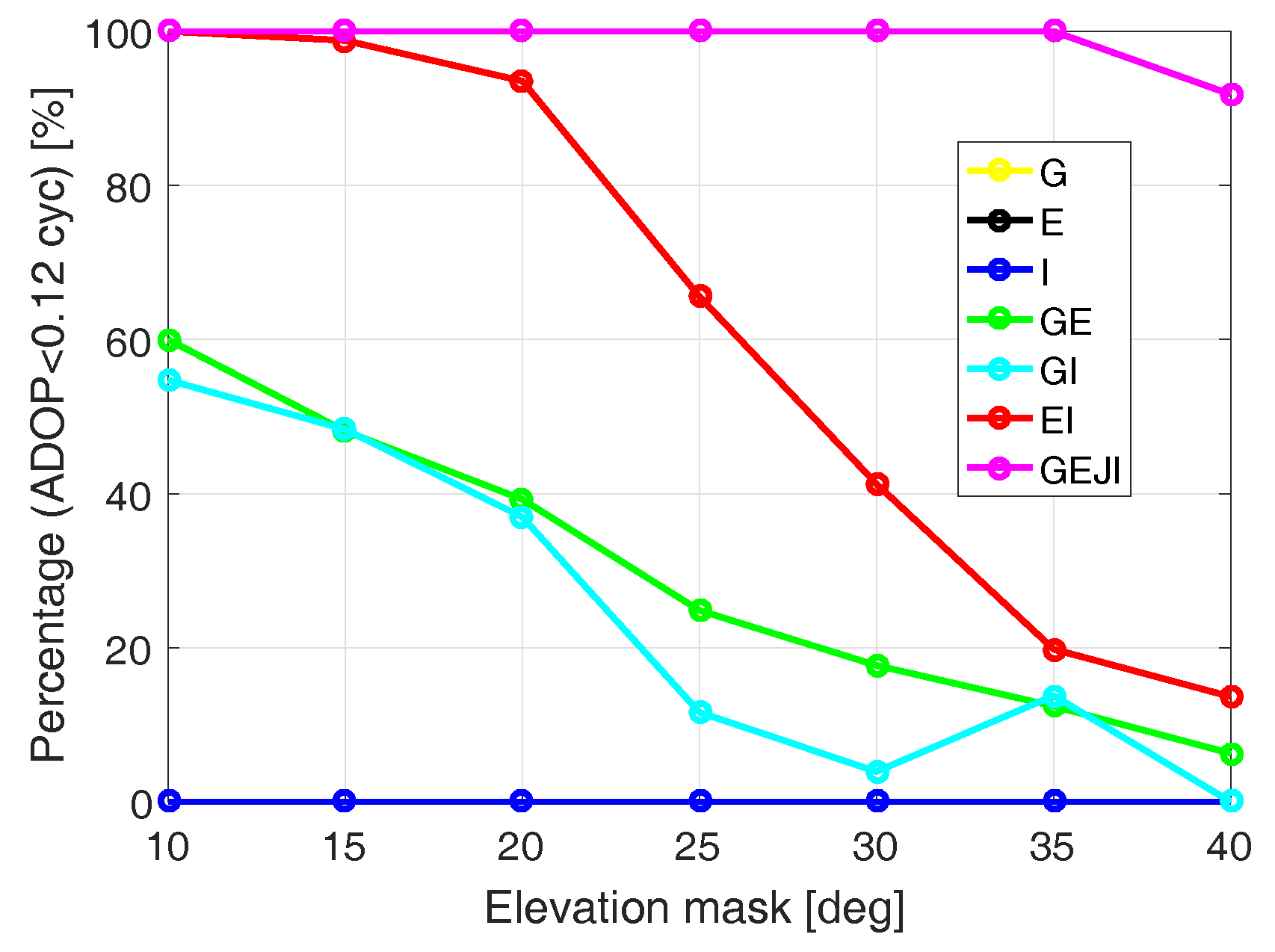
Figure 6.
Percentages within a 24 h period that ADOP is smaller than 0.12 cycles for baseline CUAA-CUCC on DOY 224, 2018. Note that the yellow and the black lines are overwritten by the blue line. The data sampling rate is 1 Hz. The yellow and black lines are overwritten by the blue line.
Figure 6.
Percentages within a 24 h period that ADOP is smaller than 0.12 cycles for baseline CUAA-CUCC on DOY 224, 2018. Note that the yellow and the black lines are overwritten by the blue line. The data sampling rate is 1 Hz. The yellow and black lines are overwritten by the blue line.
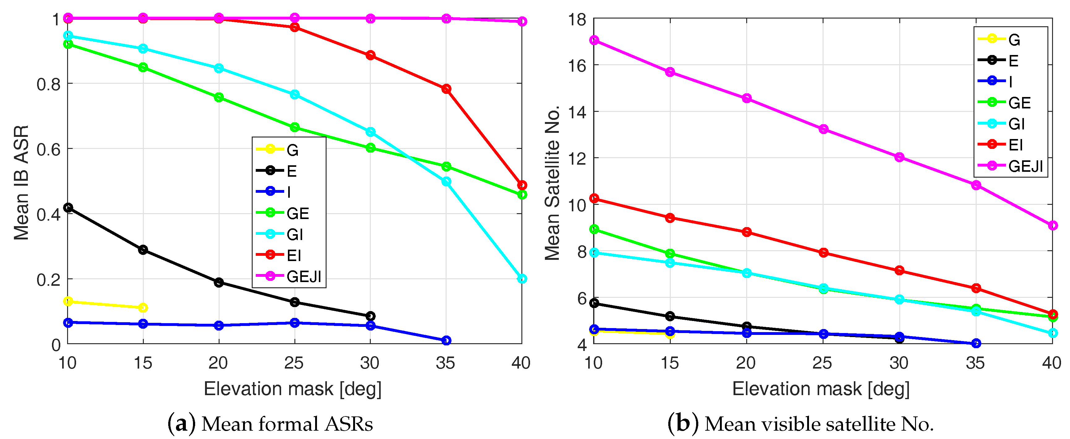
Figure 7.
Mean formal IB ASRs (a) and the corresponding mean visible satellite numbers (b) for baseline CUAA-CUCC on DOY 224, 2018. The data sampling rate is 1 Hz.
Figure 7.
Mean formal IB ASRs (a) and the corresponding mean visible satellite numbers (b) for baseline CUAA-CUCC on DOY 224, 2018. The data sampling rate is 1 Hz.
Figure 8.
Mean formal IB ASRs for short baselines from 40 E to 160 E and from 50 S to 50 N on DOY 224, 2018. The data sampling interval is 30 s.
Figure 8.
Mean formal IB ASRs for short baselines from 40 E to 160 E and from 50 S to 50 N on DOY 224, 2018. The data sampling interval is 30 s.
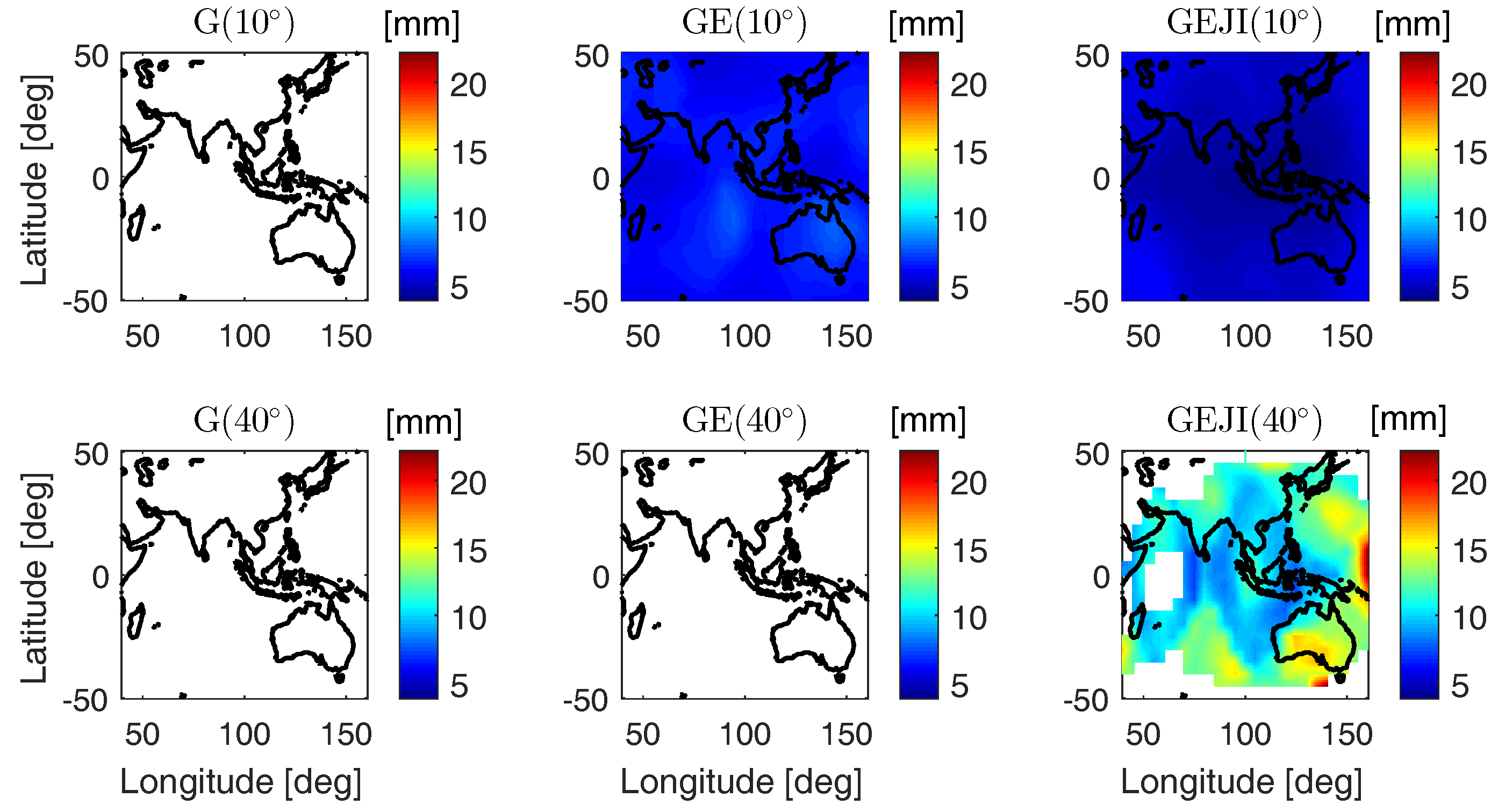
Figure 9.
Average formal standard deviations of the ambiguity-float height errors on DOY 224, 2018. The data sampling interval is 30 s.
Figure 9.
Average formal standard deviations of the ambiguity-float height errors on DOY 224, 2018. The data sampling interval is 30 s.
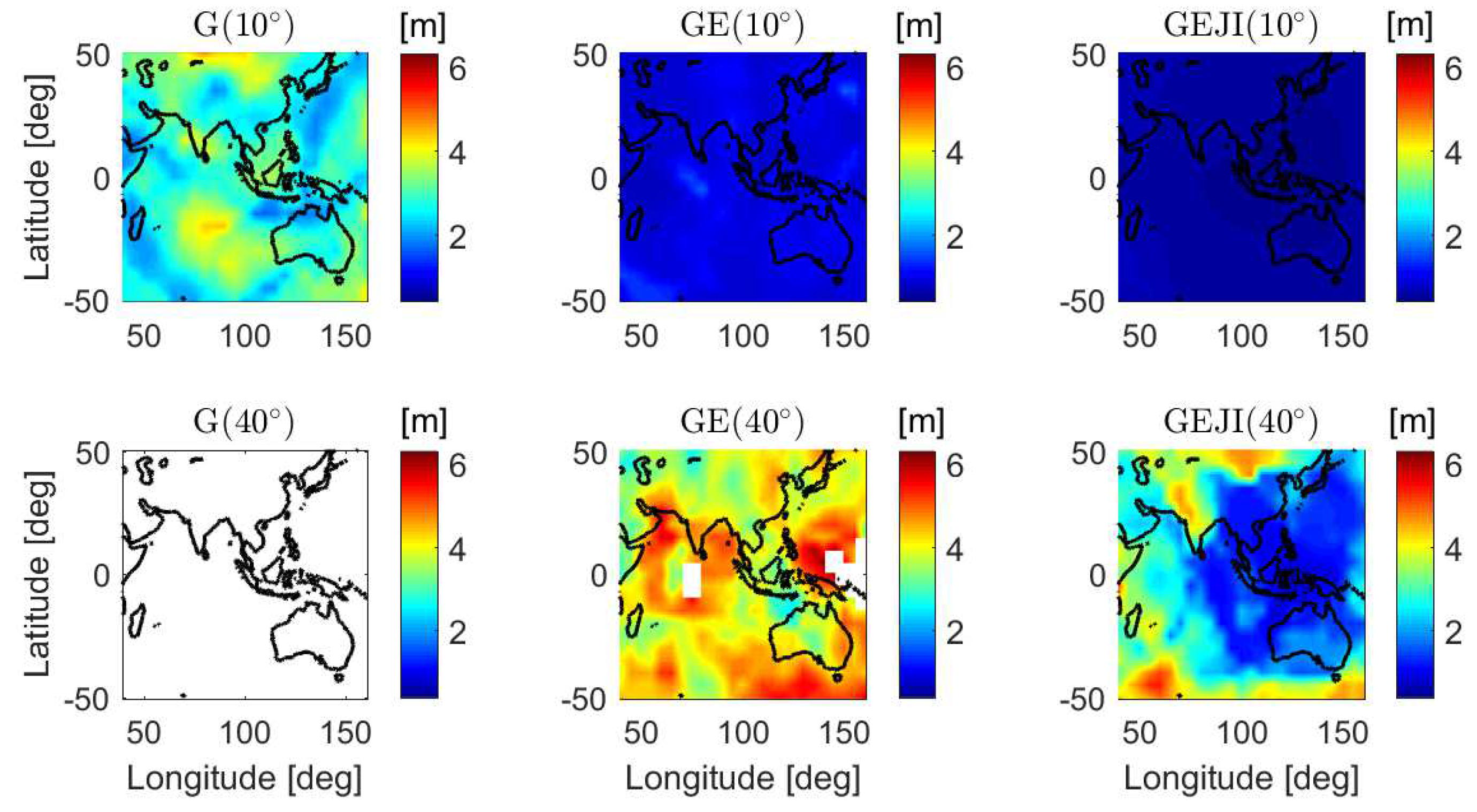
Figure 10.
Average formal standard deviations of the ambiguity-fixed height errors on DOY 224, 2018. The data sampling interval is 30 s.
Figure 10.
Average formal standard deviations of the ambiguity-fixed height errors on DOY 224, 2018. The data sampling interval is 30 s.
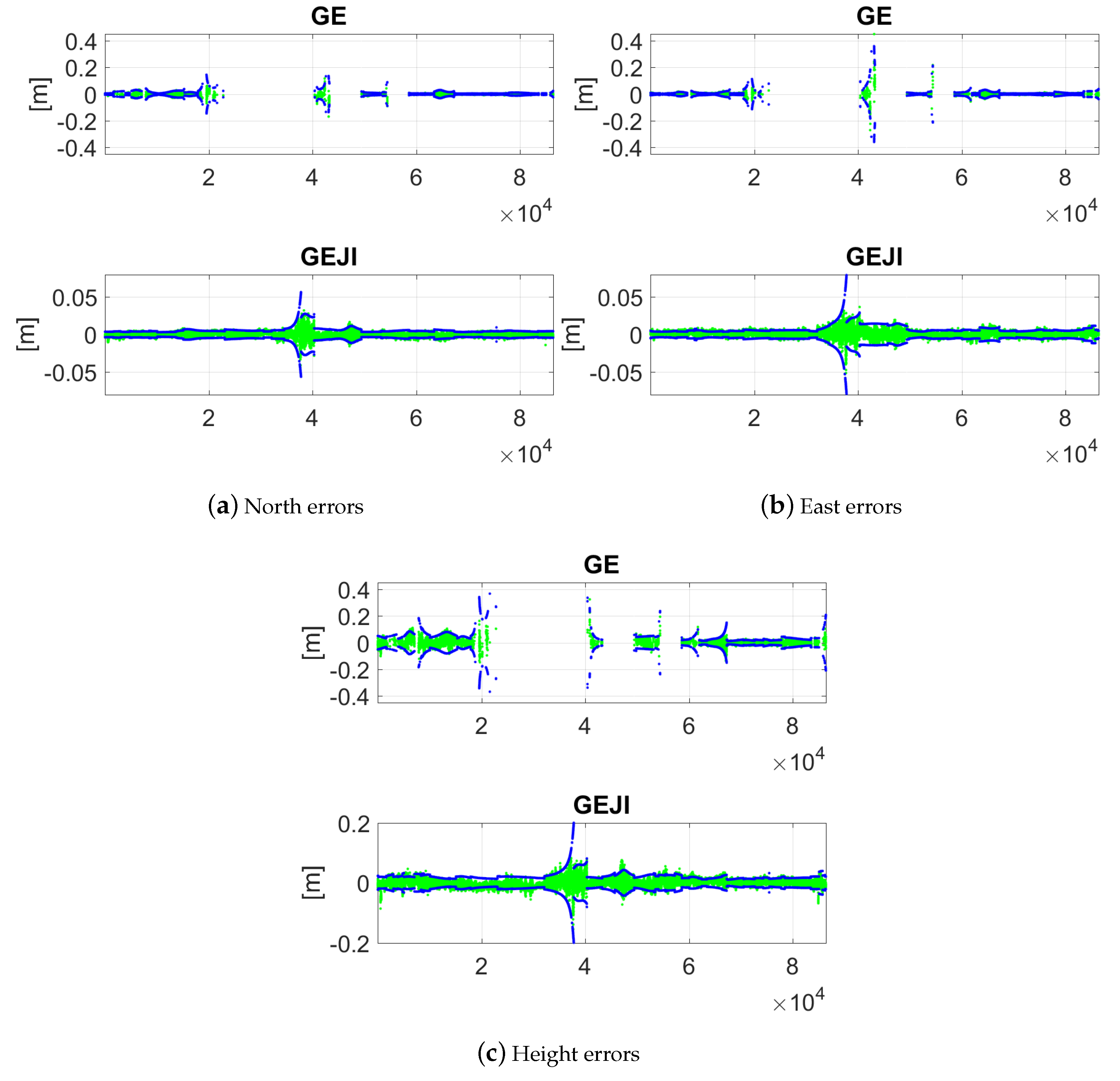
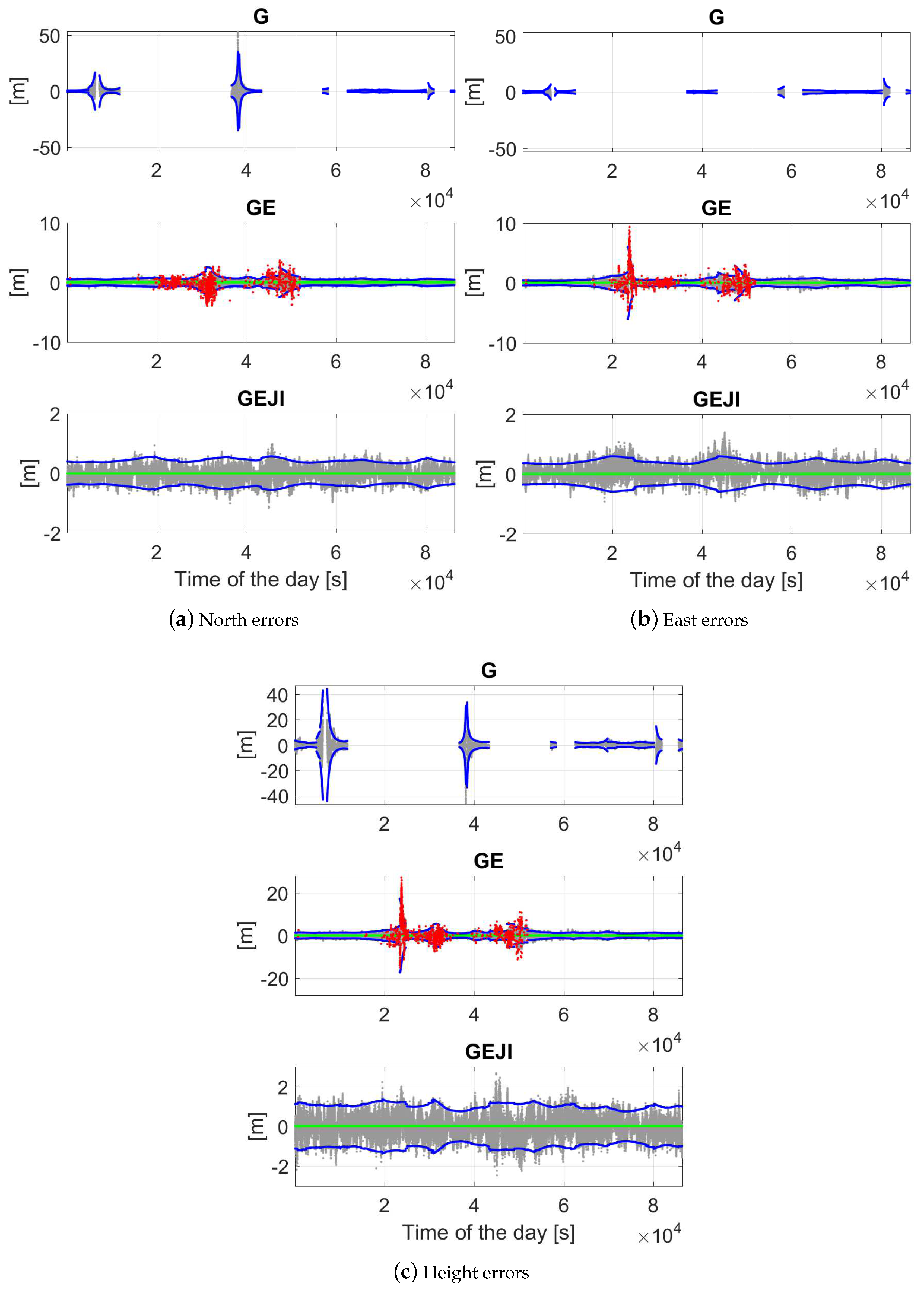
Figure 11.
Baseline errors in the north (a); east (b); and height (c) directions with the elevation mask of 10 degrees. Data for baseline CUAA-CUCC on DOY 224, 2018 was used. The gray and blue dots are the ambiguity-float solutions and their 95% formal confidence intervals, respectively. For combined solutions, the green and red dots illustrate the ambiguity-correctly-fixed and -wrongly-fixed solutions, respectively. Note that the scales of the sub-figures are different.
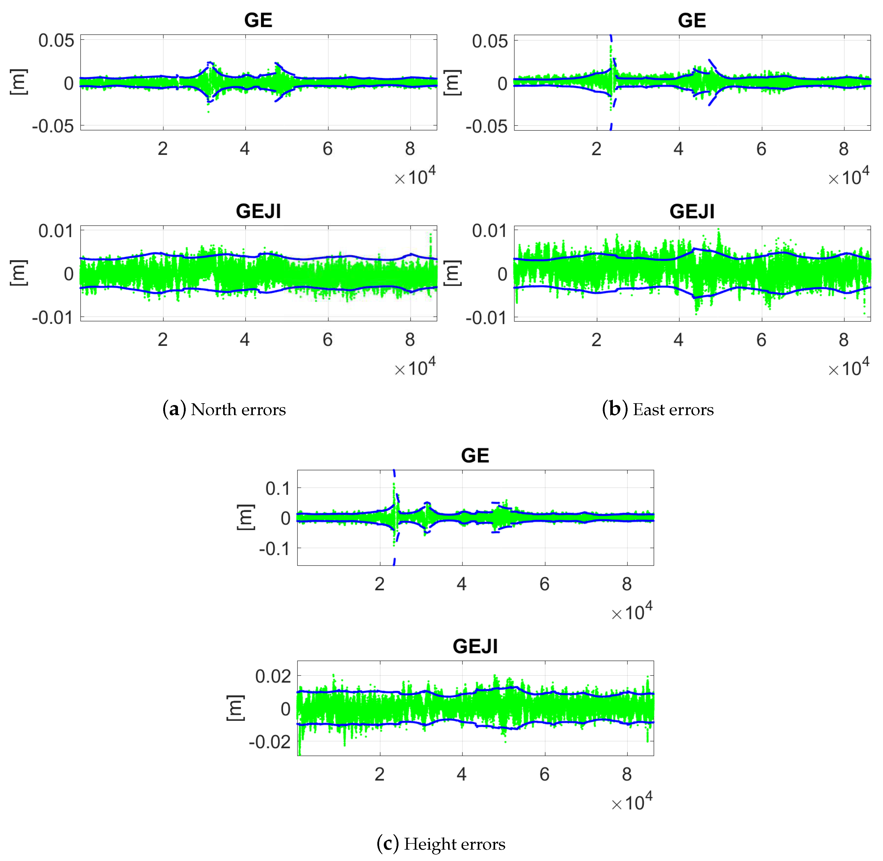
Figure 12.
Ambiguity-fixed baseline errors in the north (a); east (b); and height (c) directions with the elevation mask of 10 degrees. Data for baseline CUAA-CUCC on DOY 224, 2018 was used. The green and blue dots are the ambiguity-correctly-fixed solutions and their 95% formal confidence intervals, respectively. Note that the scales of the sub-figures are different.
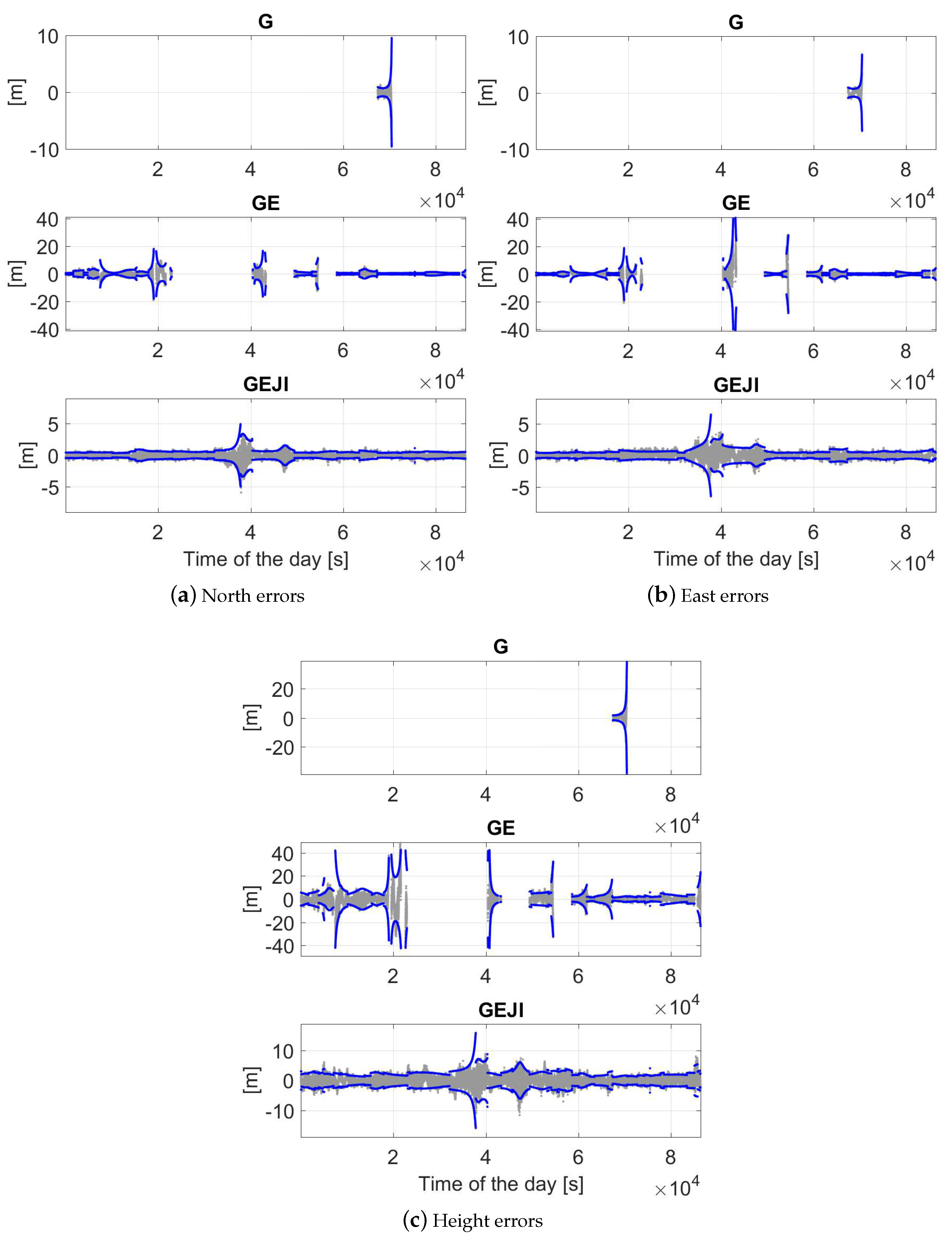
Figure 13.
Ambiguity-float baseline errors in the north (a); east (b); and height (c) directions with the elevation mask of 40 degrees. Data for baseline CUAA-CUCC on DOY 224, 2018 was used. The gray and blue dots are the ambiguity-float solutions and their 95% formal confidence intervals, respectively. Note that the scales of the sub-figures are different.
Figure 14.
Ambiguity-fixed baseline errors in the north (a); east (b); and height (c) directions with the elevation mask of 40 degrees. Data for baseline CUAA-CUCC on DOY 224, 2018 was used. The green and blue dots are the ambiguity-correctly-fixed solutions and their 95% formal confidence intervals, respectively. Note that the scales of the sub-figures are different.
Figure 15.
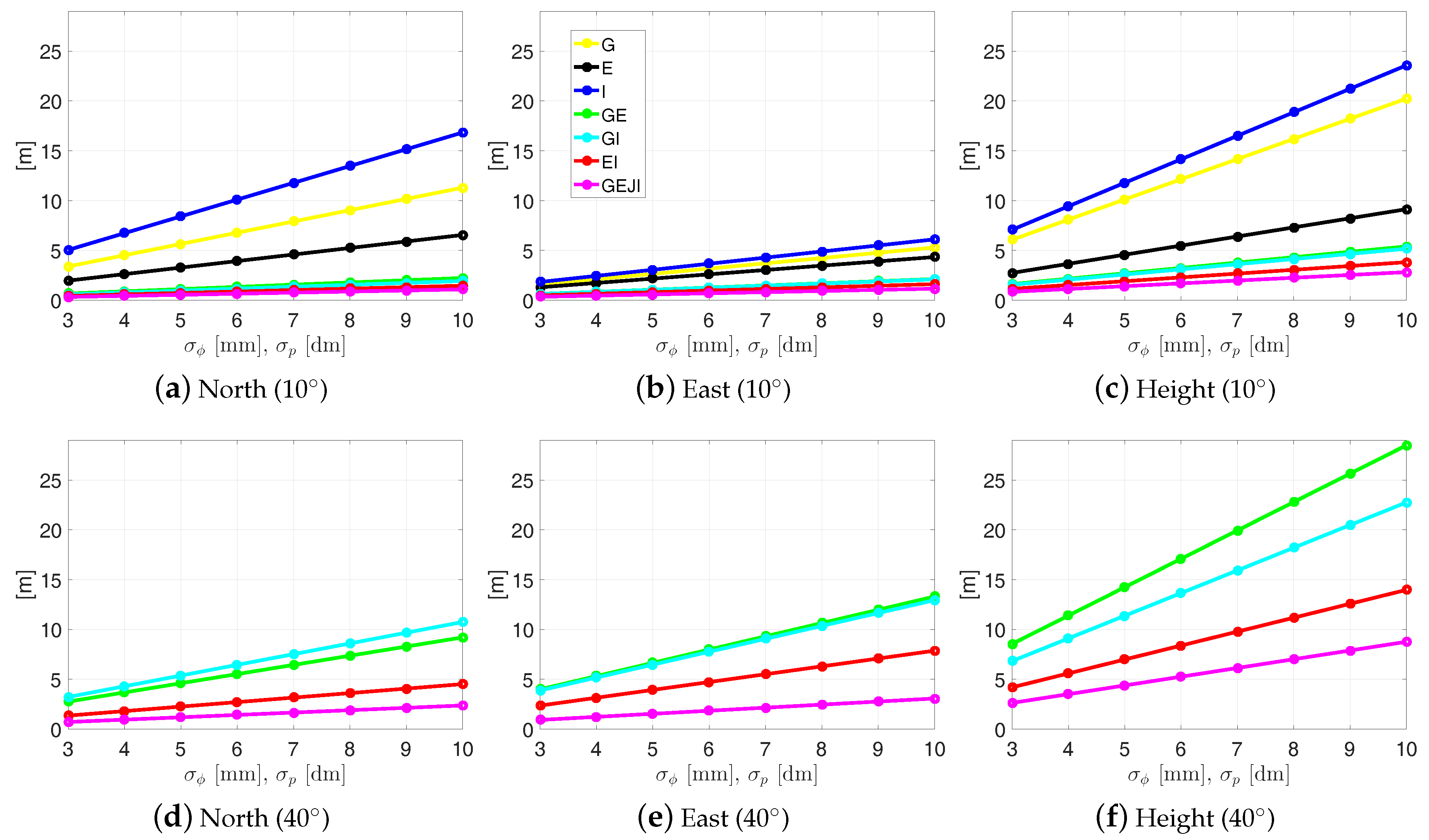
Average ambiguity-float formal standard deviations of the baseline errors for CUAU-CUCU on DOY 224, 2018. The elevation mask was set to be 10 (a–c) and 40 degrees (d–f). Note that the sub-figures have different scales.
Figure 15.
Average ambiguity-float formal standard deviations of the baseline errors for CUAU-CUCU on DOY 224, 2018. The elevation mask was set to be 10 (a–c) and 40 degrees (d–f). Note that the sub-figures have different scales.
Table 1.
L5 multipath-uncorrected phase () and code standard deviations () for GPS, Galileo, QZSS and IRNSS satellites. The standard deviations are given for elevation masks of 10/40 degrees. The data on DOY 223 was used for computing the standard deviations for GPS, Galileo and IRNSS, and the data on DOY 153, 2018 was used for computing the QZSS standard deviations.
| System | CUAA-CUCC | CUAA-CUBB |
|---|
| [mm] | [cm] | [mm] | [cm] |
|---|
| GPS | 2/1 | 17/15 | 2/1 | 17/14 |
| Galileo | 2/1 | 19/17 | 2/1 | 18/15 |
| QZSS | 2/2 | 14/13 | 2/2 | 16/15 |
| IRNSS | 2/1 | 25/21 | 2/1 | 26/26 |
Table 2.
Empirical and average formal IB ASRs (in brackets). The data of baseline CUAA-CUCC and CUAA-CUBB on DOY 224, 2018 was used.
Table 2.
Empirical and average formal IB ASRs (in brackets). The data of baseline CUAA-CUCC and CUAA-CUBB on DOY 224, 2018 was used.
| System ID | CUAA-CUCC | CUAA-CUBB |
|---|
| Elevation Mask | 10 | 25 | 40 | 10 | 25 | 40 |
|---|
| G | 0.151(0.130) | – | – | 0.160(0.132) | – | – |
| E | 0.458(0.411) | 0.129(0.128) | – | 0.484(0.441) | 0.158(0.151) | – |
| I | 0.050(0.066) | 0.041(0.064) | – | 0.058(0.059) | 0.054(0.055) | – |
| G/E | 0.925(0.906) | 0.692(0.664) | 0.489(0.457) | 0.915(0.909) | 0.687(0.682) | 0.516(0.488) |
| G/I | 0.925(0.946) | 0.752(0.766) | 0.193(0.200) | 0.928(0.942) | 0.759(0.762) | 0.168(0.186) |
| E/I | 0.997(1.000) | 0.962(0.972) | 0.494(0.487) | 1.000(1.000) | 0.959(0.975) | 0.491(0.485) |
| G/E/J/I | 1.000(1.000) | 0.999(0.997) | 0.962(0.958) | 1.000(1.000) | 1.000(1.000) | 0.969(0.951) |
Table 3.
Empirical and average formal (in brackets) standard deviations of the ambiguity-float baseline errors. The results are given in the north/east/height directions. The data on DOY 224, 2018 was used for both baselines.
Table 3.
Empirical and average formal (in brackets) standard deviations of the ambiguity-float baseline errors. The results are given in the north/east/height directions. The data on DOY 224, 2018 was used for both baselines.
| System ID | CUAA-CUCC [dm] | CUAA-CUBB [dm] |
|---|
| Elevation Mask | 10 | 40 | 10 | 40 |
|---|
| G | 22(19)/7(9)/31(34) | – | 18(19)/7(9)/30(35) | – |
| E | 9(13)/9(9)/21(21) | – | 11(12)/9(8)/20(20) | – |
| I | 37(41)/14(15)/51(58) | – | 43(44)/16(16)/60(61) | – |
| G/E | 4(4)/5(5)/13(12) | 16(15)/21(21)/48(45) | 4(4)/4(5)/11(12) | 14(14)/24(20)/38(43) |
| G/I | 4(4)/5(5)/11(11) | 24(20)/21(23)/47(45) | 4(4)/5(5)/13(12) | 29(24)/26(27)/55(53) |
| E/I | 3(3)/4(3)/7(8) | 7(9)/11(15)/27(28) | 3(3)/4(3)/8(8) | 8(10)/13(17)/31(32) |
| G/E/J/I | 2(2)/2(2)/5(5) | 4(4)/5(5)/14(15) | 2(2)/2(2)/5(5) | 4(5)/5(6)/15(17) |
Table 4.
Empirical and average formal (in brackets) standard deviations of the ambiguity-fixed baseline errors. The results are given in the north/east/height directions. The data on DOY 224, 2018 was used for both baselines.
Table 4.
Empirical and average formal (in brackets) standard deviations of the ambiguity-fixed baseline errors. The results are given in the north/east/height directions. The data on DOY 224, 2018 was used for both baselines.
| System ID | CUAA-CUCC [mm] | CUAA-CUBB [mm] |
|---|
| Elevation Mask | 10 | 40 | 10 | 40 |
|---|
| E | 3(4)/4(4)/9(10) | – | 3(4)/4(4)/9(10) | – |
| G/E | 3(3)/3(4)/7(9) | 6(8)/8(9)/19(24) | 3(3)/3(3)/8(8) | 6(7)/8(8)/18(22) |
| G/I | 3(3)/3(3)/7(8) | – | 3(3)/3(3)/7(8) | – |
| E/I | 2(2)/3(3)/6(6) | 3(4)/5(6)/16(19) | 2(2)/3(3)/6(6) | 3(4)/4(5)/15(16) |
| G/E/J/I | 2(2)/2(2)/5(5) | 3(4)/3(5)/11(13) | 2(2)/2(2)/4(5) | 3(3)/3(4)/10(12) |
Table 5.
Average ambiguity-fixed formal standard deviations of the baseline errors for CUAU-CUCU in Galileo/IRNSS and GPS/Galileo/QZSS/IRNSS-combined cases. The MGEX combined broadcast ephemeris on DOY 224, 2018 was used for the computation. The standard deviations (STD) are given in the format of North/East/Up directions.
| Signal STD | E/I [mm] | G/E/J/I [mm] |
|---|
| Elevation Mask | 10 |
| = 3 mm, = 3 dm | 4/5/12 | 3/3/8 |
| = 4 mm, = 4 dm | – | 4/5/11 |
| = 5 mm, = 5 dm | – | 5/6/14 |
| Elevation mask | 40 |
| = 3 mm, = 3 dm | – | 4/5/19 |


