A Polydimethylsiloxane (PDMS) Waveguide Sensor that Mimics a Neuromast to Measure Fluid Flow Velocity †

 , and
, and 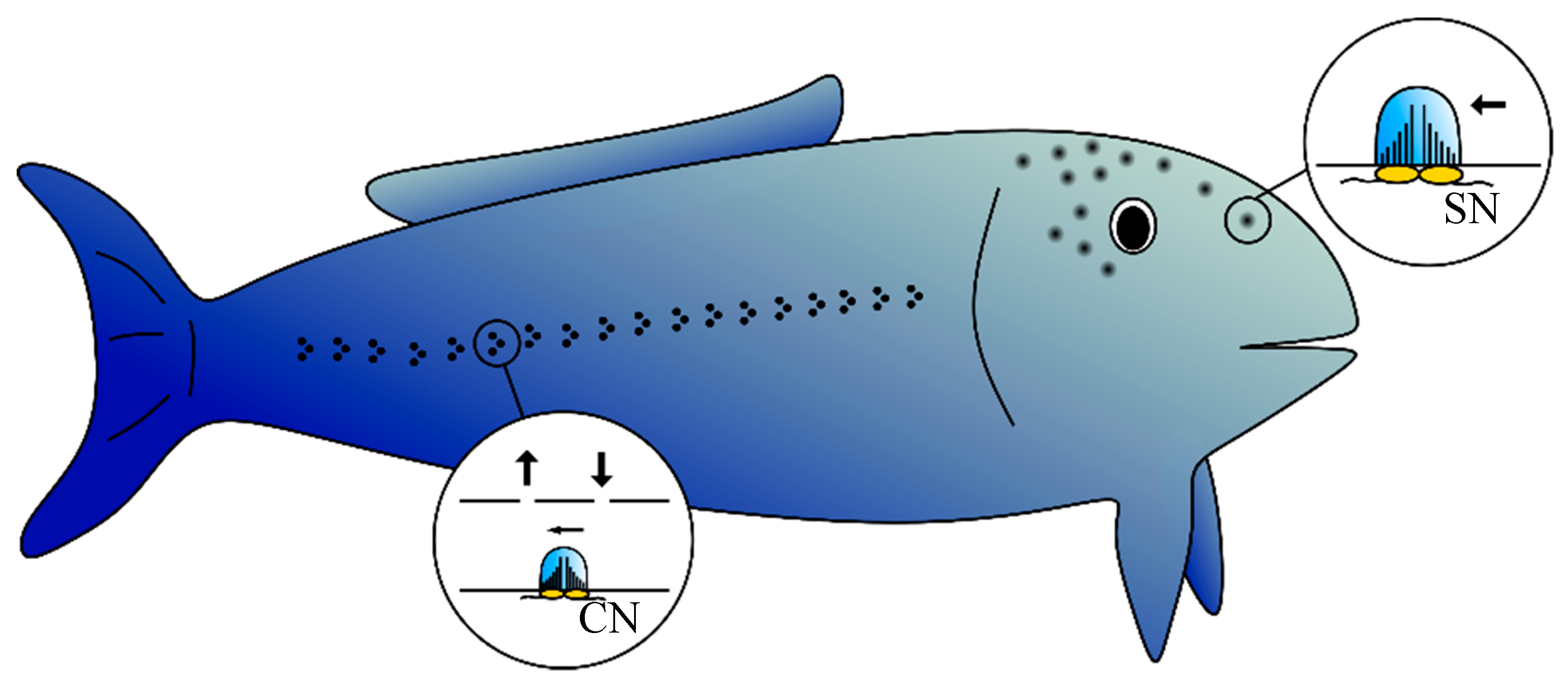
Abstract
1. Introduction
2. Materials and Methods
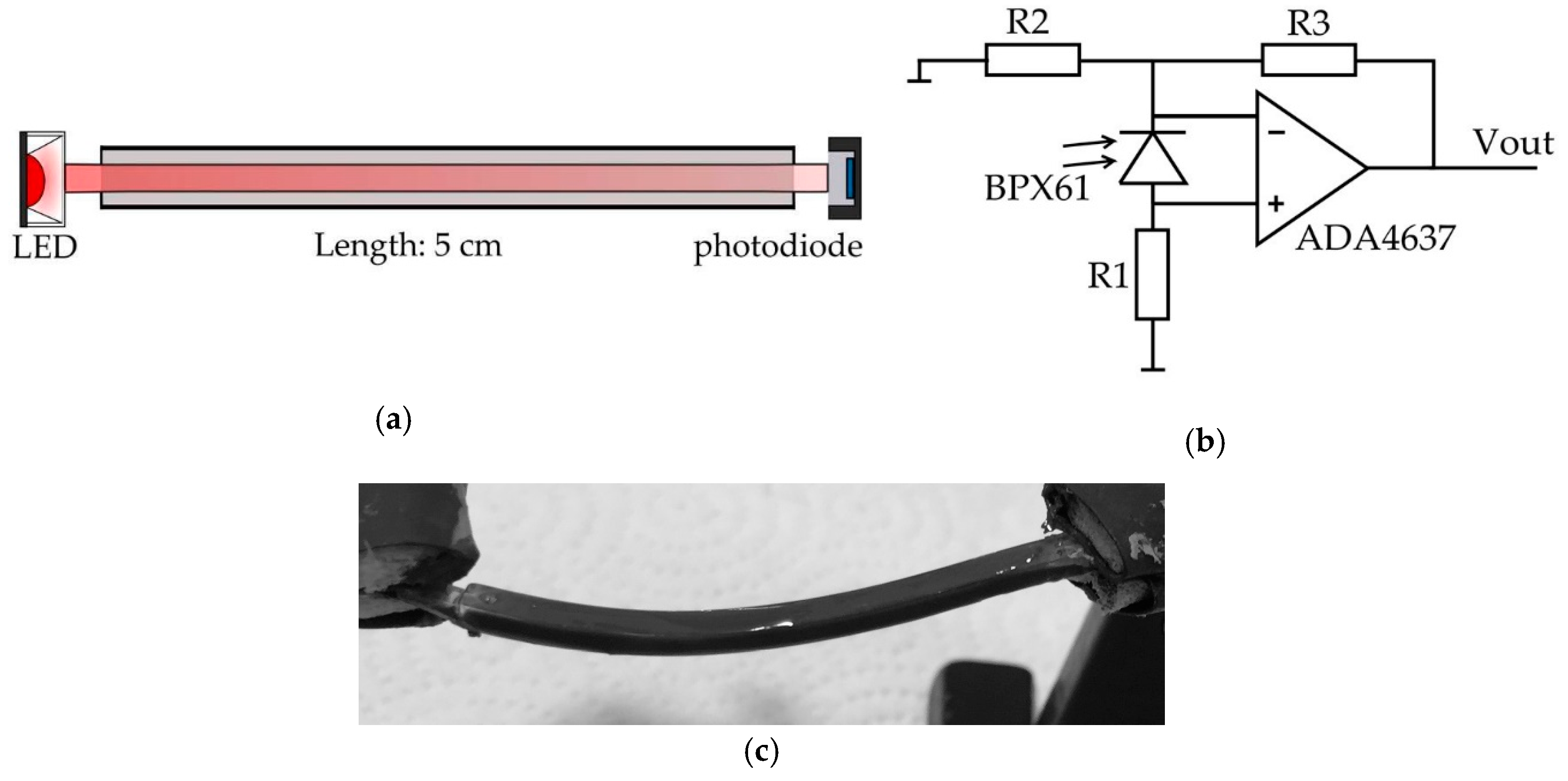
2.1. PDMS Waveguide
2.2. Photodiode and Photodiode Amplifier
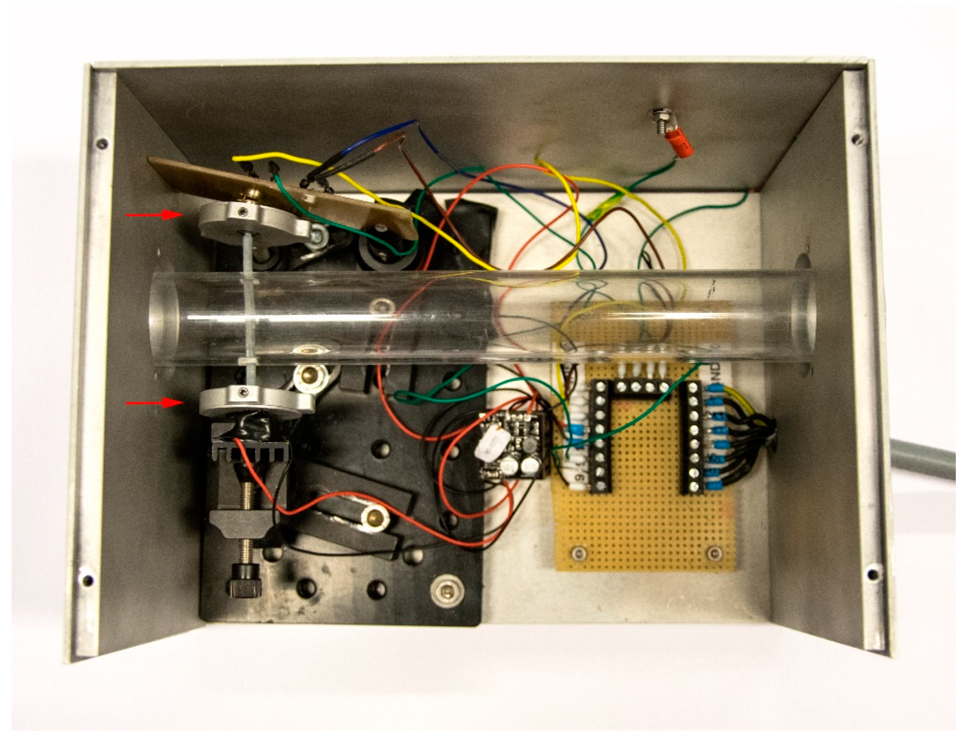
2.3. Measurement Setup
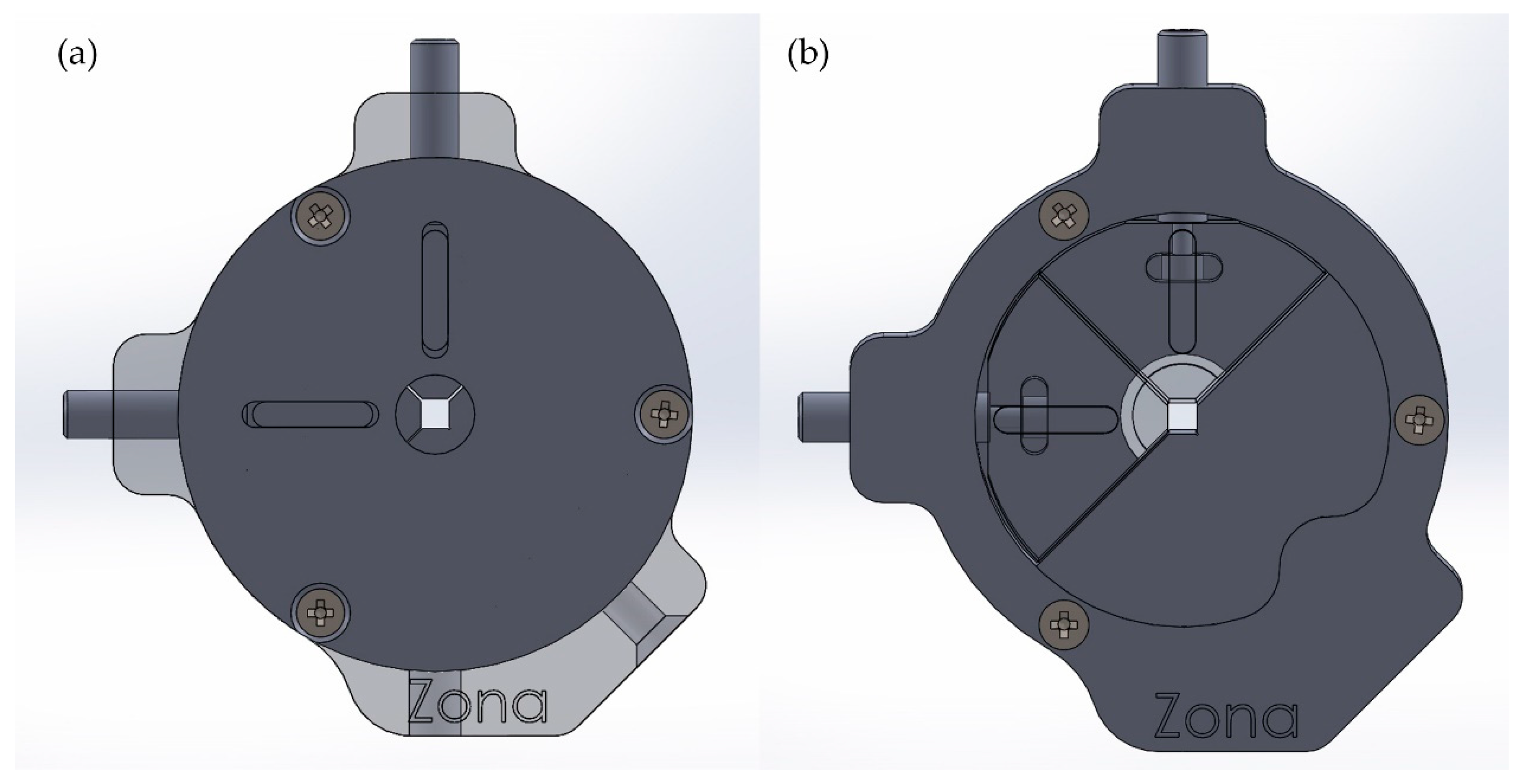
2.3.1. Setup 1: Bending Masses Simulate Fiber Deflection
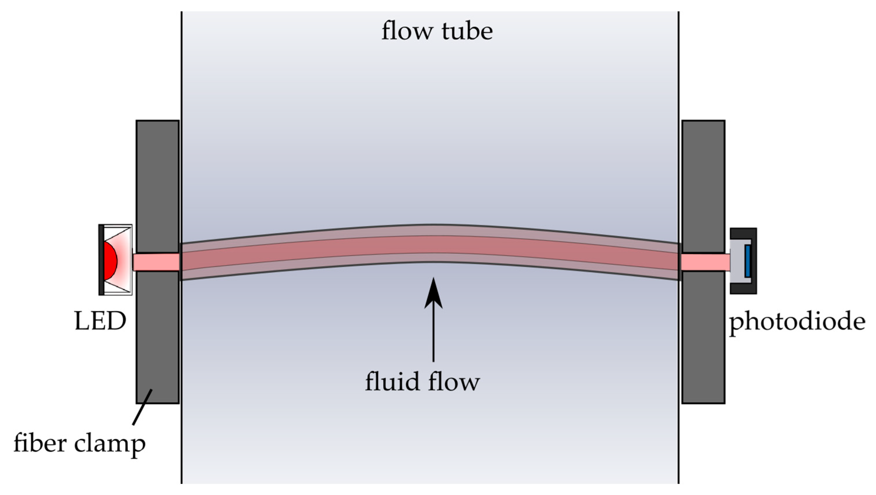
2.3.2. Setup 2: Fluid Flow Measurements
3. Results and Discussion
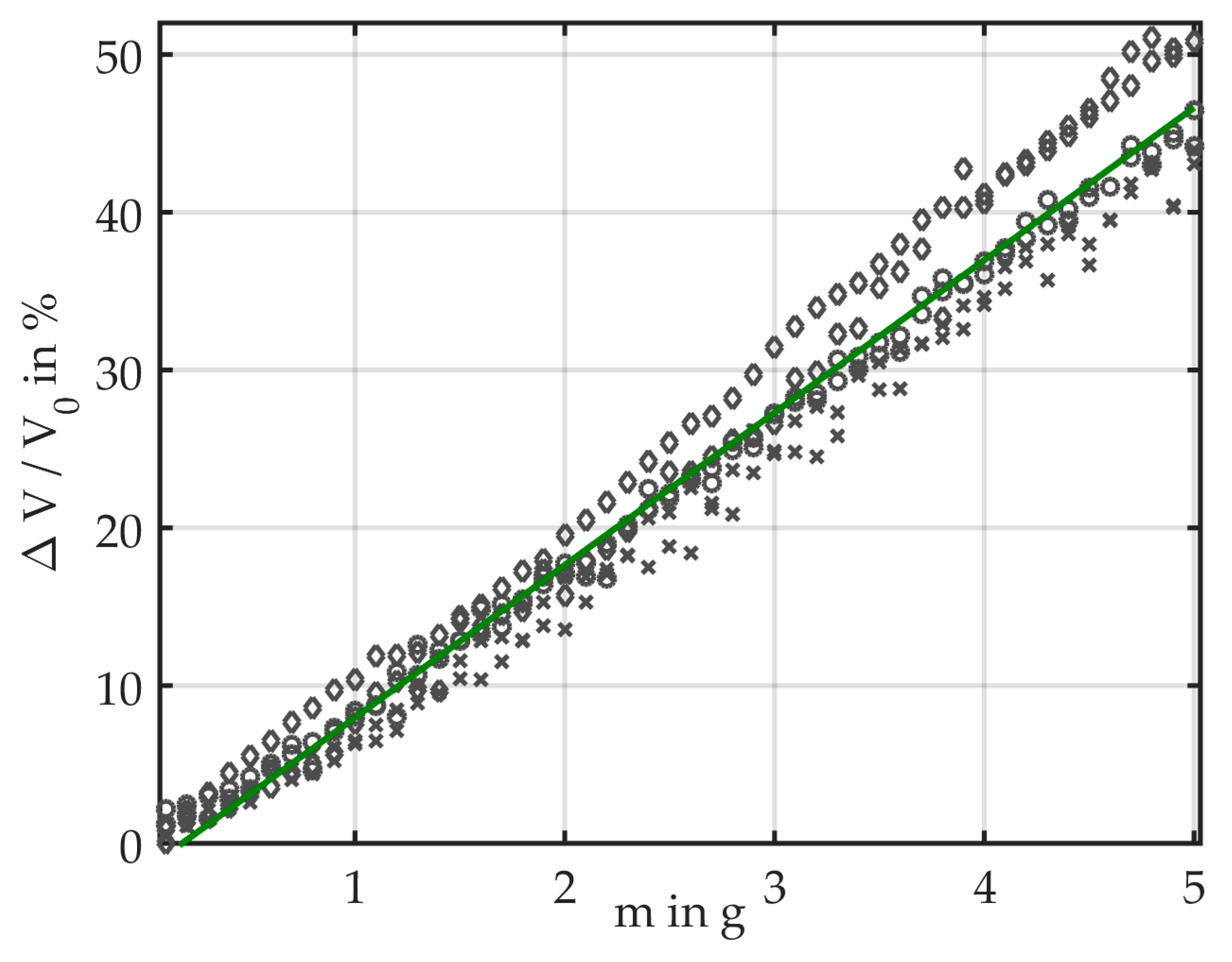
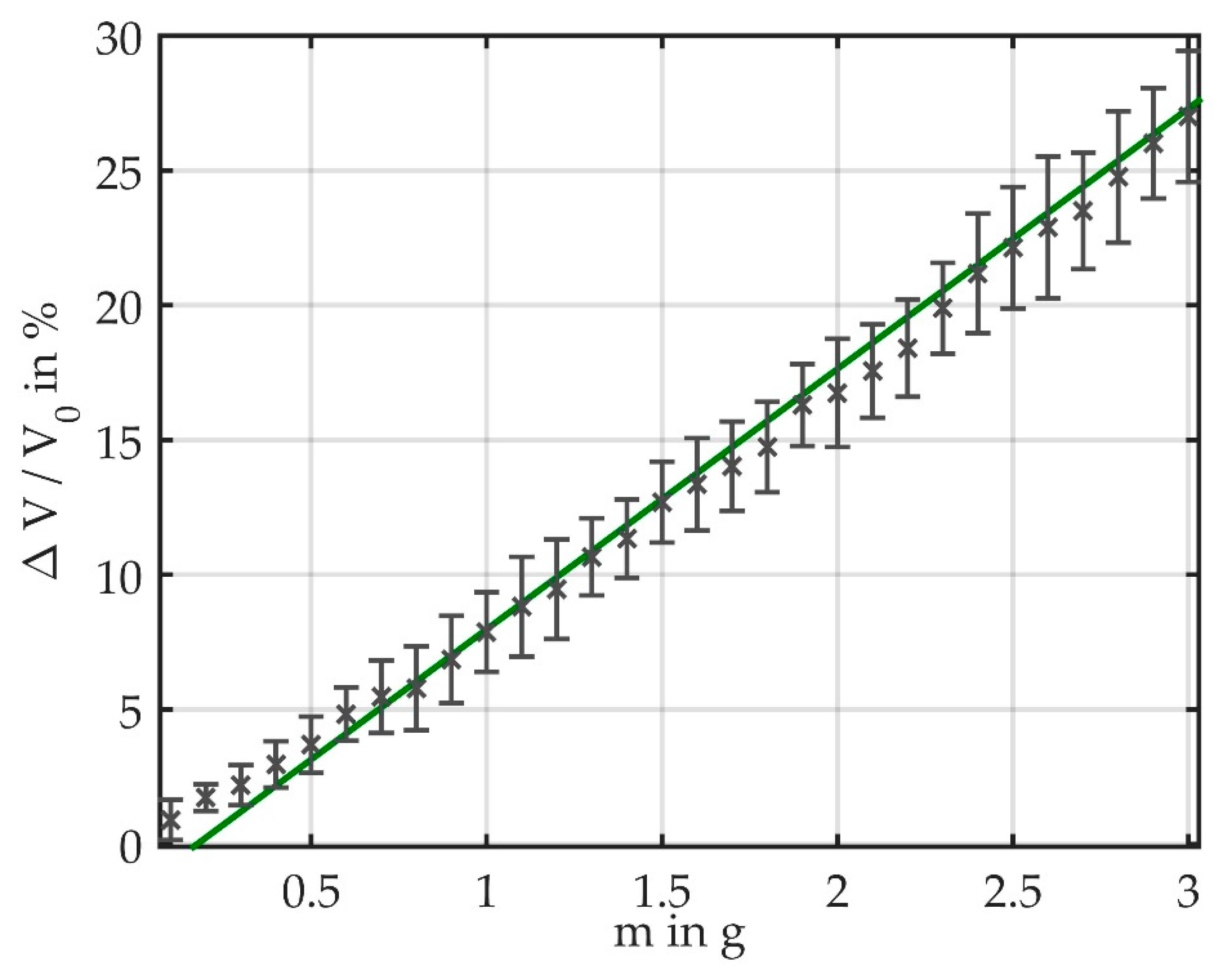
3.1. Bending Induced by Masses
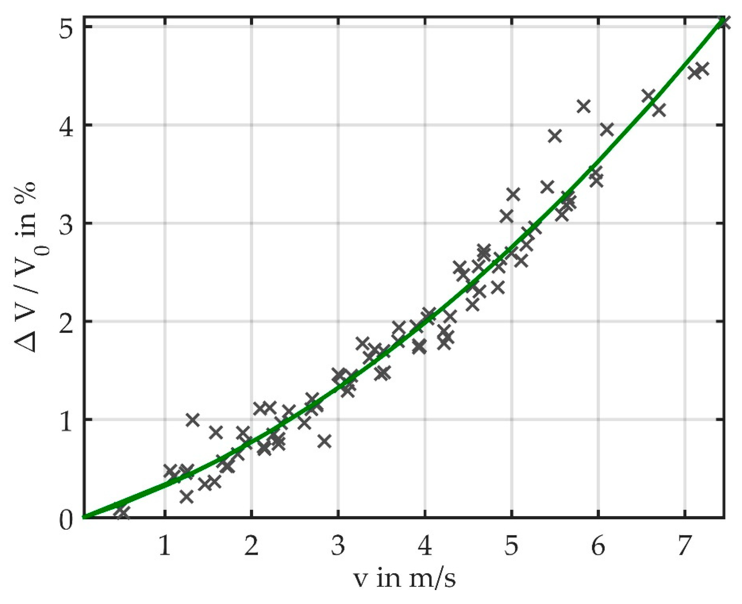
3.2. Exposing Fiber to Air Flow
3.3. Comparison of the Measurement Setups
3.4. Fluid Flow around an Elastic Fiber
4. Conclusions
Author Contributions
Funding
Acknowledgments
Conflicts of Interest
References
- Benyus, J.M. Biomimicry: Innovation Inspired by Nature; HarperCollins: New York, NY, USA, 2002. [Google Scholar]
- Wiesmayr, B. Bioinspired Flow Sensor and Its Application in Spirometry. Master’s Thesis, Universität Linz, Linz, Austria, 2018. [Google Scholar]
- Bleckmann, H.; Zelick, R. Lateral line system of fish. Integr. Zool. 2009, 4, 13–25. [Google Scholar] [CrossRef] [PubMed]
- Mogdans, J.; Bleckmann, H. Coping with flow: Behavior, neurophysiology and modeling of the fish lateral line system. Biol. Cybern. 2012, 106, 627–642. [Google Scholar] [CrossRef] [PubMed]
- Coombs, S.; Montgomery, J.C. The Enigmatic Lateral Line System. In Comparative Hearing: Fish and Amphibians; Fay, R.R., Popper, A.N., Eds.; Springer: New York, NY, USA, 1999; Volume 11, pp. 319–362. [Google Scholar]
- Yang, Y.; Chen, J.; Engel, J.; Pandya, S.; Chen, N.; Tucker, C.; Coombs, S.; Jones, D.L.; Liu, C. Distant touch hydrodynamic imaging with an artificial lateral line. Proc. Natl. Acad. Sci. USA 2006, 103, 18891–18895. [Google Scholar] [CrossRef] [PubMed]
- Izadi, N.; de Boer, M.J.; Berenschot, J.W.; Krijnen, G.J.M. Fabrication of superficial neuromast inspired capacitive flow sensors. J. Micromech. Microeng. 2010, 20, 85041. [Google Scholar] [CrossRef]
- Asadnia, M.; Kottapalli, A.G.P.; Miao, J.; Warkiani, M.E.; Triantafyllou, M.S. Artificial fish skin of self-powered micro-electromechanical systems hair cells for sensing hydrodynamic flow phenomena. J. R. Soc. Interface 2015, 12, 20150322. [Google Scholar] [CrossRef] [PubMed]
- Abdulsadda, A.T.; Tan, X. An artificial lateral line system using IPMC sensor arrays. Int. J. Smart Nano Mater. 2012, 3, 226–242. [Google Scholar] [CrossRef]
- Herzog, H.; Klein, A.; Bleckmann, H.; Holik, P.; Schmitz, S.; Siebke, G.; Tätzner, S.; Lacher, M.; Steltenkamp, S. Micro-biomimetic flow sensors—Introducing light-guiding PDMS structures into MEMS. Bioinspir. Biomim. 2015, 10, 36001. [Google Scholar] [CrossRef] [PubMed]
- Herzog, H.; Steltenkamp, S.; Klein, A.; Tätzner, S.; Schulze, E.; Bleckmann, H. Micro-Machined Flow Sensors Mimicking Lateral Line Canal Neuromasts. Micromachines 2015, 6, 1189–1212. [Google Scholar] [CrossRef]
- Yang, Y.; Klein, A.; Bleckmann, H.; Liu, C. Artificial lateral line canal for hydrodynamic detection. Appl. Phys. Lett. 2011, 99, 23701. [Google Scholar] [CrossRef]
- Klein, A.T.; Kaldenbach, F.; Rüter, A.; Bleckmann, H. What We Can Learn from Artificial Lateral Line Sensor Arrays. Adv. Exp. Med. Biol. 2016, 875, 539–545. [Google Scholar] [PubMed]
- Chen, J.; Engel, J.; Chen, N.; Pandya, S.; Coombs, S.; Liu, C. Artificial Lateral Line and Hydrodynamic Object Tracing. In Proceedings of the 19th IEEE International Conference on Micro Electro Mechanical Systems, Istanbul, Turkey, 22–26 January 2006. [Google Scholar]
- Nguyen, N.; Jones, D.L.; Yang, Y.; Liu, C. Flow Vision for Autonomous Underwater Vehicles via an Artificial Lateral Line. Eurasip J. Adv. Signal Process. 2011, 2011, 9. [Google Scholar] [CrossRef]
- Stadler, A.T.; Pavlicek, P.; Baumgartner, W. Bio-inspired flow sensor: Mimicking the lateral line organ with an optical sensory system. In Proceedings of the Bioeng’15, Istanbul, Turkey, 27–30 July 2015. [Google Scholar]
- Stadler, A.T.; Wiesmayr, B.; Krieger, M.; Baumgartner, W. An optical sensory principle for spirometry. Presented at Sensoren und Messsysteme 2018: 19. ITG-/GMA-Fachtagung. In Sensoren und Messsysteme: Beiträge der 19. ITG/GMA-Fachtagung 26.-27. Juni 2018 in Nürnberg; Reindl, L.M., Ed.; VDE Verlag GmbH: Berlin, Germany, 2018; Volume 281. [Google Scholar]
- Horowitz, P.; Hill, W. The Art of Electronics, 3rd ed.; Cambridge University Press: Cambridge, UK; New York, NY, USA, 2015. [Google Scholar]
- Schneider, F.; Draheim, J.; Kamberger, R.; Wallrabe, U. Process and material properties of polydimethylsiloxane (PDMS) for Optical MEMS. Sens. Actuators A Phys. 2009, 151, 95–99. [Google Scholar] [CrossRef]
- Snyder, A.W.; Love, J.D. Optical Waveguide Theory; Springer: Boston, MA, USA, 1983. [Google Scholar]
- Osram Opto Semiconductors. Silicon PIN Photodiode BPX61, Data Sheet, 1st ed.; Osram Opto Semiconductors: Regensburg, Germany, 2018. [Google Scholar]
- Analog Devices. ADA4627-1/ADA4637-1: 30 V, High Speed, Low Noise, Low Bias Current JFET Operational Amplifier; Data Sheet; Analog Devices: Norwood, MA, USA, 2015. [Google Scholar]
- Anderson, J.D. Fundamentals of Aerodynamics, 6th ed.; McGraw-Hill Education: Berkshire, UK, 2016. [Google Scholar]
- Williamson, C.H.K. Vortex Dynamics in the Cylinder Wake. Annu. Rev. Fluid Mech. 1996, 28, 477–539. [Google Scholar] [CrossRef]
- Brun, C.; Aubrun, S.; Goossens, T.; Ravier, P. Coherent Structures and their Frequency Signature in the Separated Shear Layer on the Sides of a Square Cylinder. Flow Turbul. Combust 2008, 81, 97–114. [Google Scholar] [CrossRef]
- Saha, A.K.; Biswas, G.; Muralidhar, K. Three-dimensional study of flow past a square cylinder at low Reynolds numbers. Int. J. Heat Fluid Flow 2003, 24, 54–66. [Google Scholar] [CrossRef]
- Okajima, A. Strouhal numbers of rectangular cylinders. J. Fluid Mech. 1982, 123, 379. [Google Scholar] [CrossRef]
- Zhao, M.; Cheng, L.; Zhou, T. Numerical simulation of vortex-induced vibration of a square cylinder at a low Reynolds number. Phys. Fluids 2013, 25, 23603. [Google Scholar] [CrossRef]


© 2019 by the authors. Licensee MDPI, Basel, Switzerland. This article is an open access article distributed under the terms and conditions of the Creative Commons Attribution (CC BY) license (http://creativecommons.org/licenses/by/4.0/).
Share and Cite
Wiesmayr, B.; Höglinger, M.; Krieger, M.; Lindner, P.; Baumgartner, W.; Stadler, A.T. A Polydimethylsiloxane (PDMS) Waveguide Sensor that Mimics a Neuromast to Measure Fluid Flow Velocity. Sensors 2019, 19, 925. https://doi.org/10.3390/s19040925
Wiesmayr B, Höglinger M, Krieger M, Lindner P, Baumgartner W, Stadler AT. A Polydimethylsiloxane (PDMS) Waveguide Sensor that Mimics a Neuromast to Measure Fluid Flow Velocity. Sensors. 2019; 19(4):925. https://doi.org/10.3390/s19040925
Chicago/Turabian StyleWiesmayr, Bianca, Markus Höglinger, Michael Krieger, Philip Lindner, Werner Baumgartner, and Anna T. Stadler. 2019. "A Polydimethylsiloxane (PDMS) Waveguide Sensor that Mimics a Neuromast to Measure Fluid Flow Velocity" Sensors 19, no. 4: 925. https://doi.org/10.3390/s19040925
APA StyleWiesmayr, B., Höglinger, M., Krieger, M., Lindner, P., Baumgartner, W., & Stadler, A. T. (2019). A Polydimethylsiloxane (PDMS) Waveguide Sensor that Mimics a Neuromast to Measure Fluid Flow Velocity. Sensors, 19(4), 925. https://doi.org/10.3390/s19040925