Feature Extraction and Classification of Citrus Juice by Using an Enhanced L-KSVD on Data Obtained from Electronic Nose


Abstract
:1. Introduction
- (a)
- The traditional L-KSVD cannot handle the problem of nonlinear data very well, and the kernel function is adopted in this paper to help L-KSVD deal with the nonlinear data obtained by the E-nose.
- (b)
- Choosing a proper dictionary is the first and most important step of L-KSVD, and a novel dictionary initialization method is proposed according to the data characteristics of the E-nose. With the help of the Enhance Quantum-behaved Particle Swarm Optimization (EQPSO), this method generates random numbers in binary and uses the recognition rate as a fitness function to decide which sensor response will be used to initialize the dictionary.
- (c)
- The weighted coefficients of the objective function of L-KSVD have a bigger impact on the classification accuracy, so these coefficients are standardized and then optimized with the help of EQPSO in this paper.
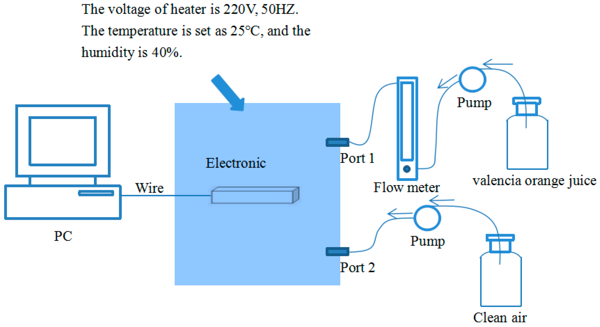
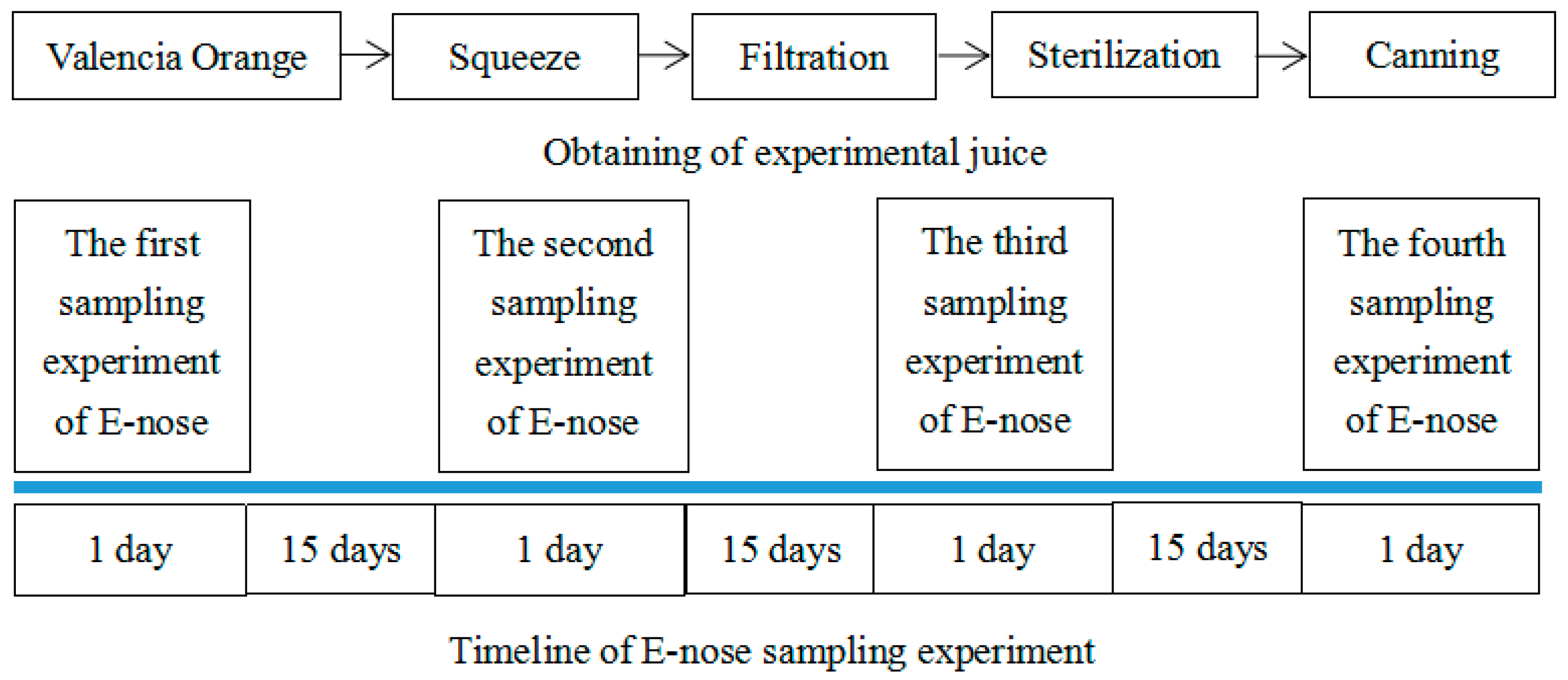
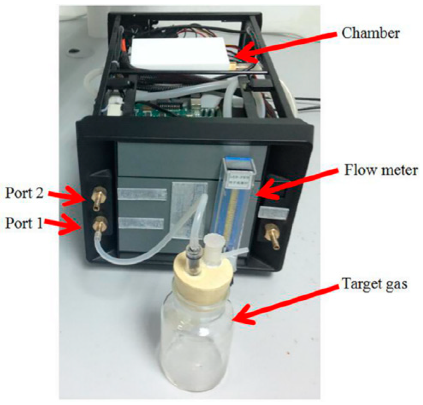
2. Materials and Methods
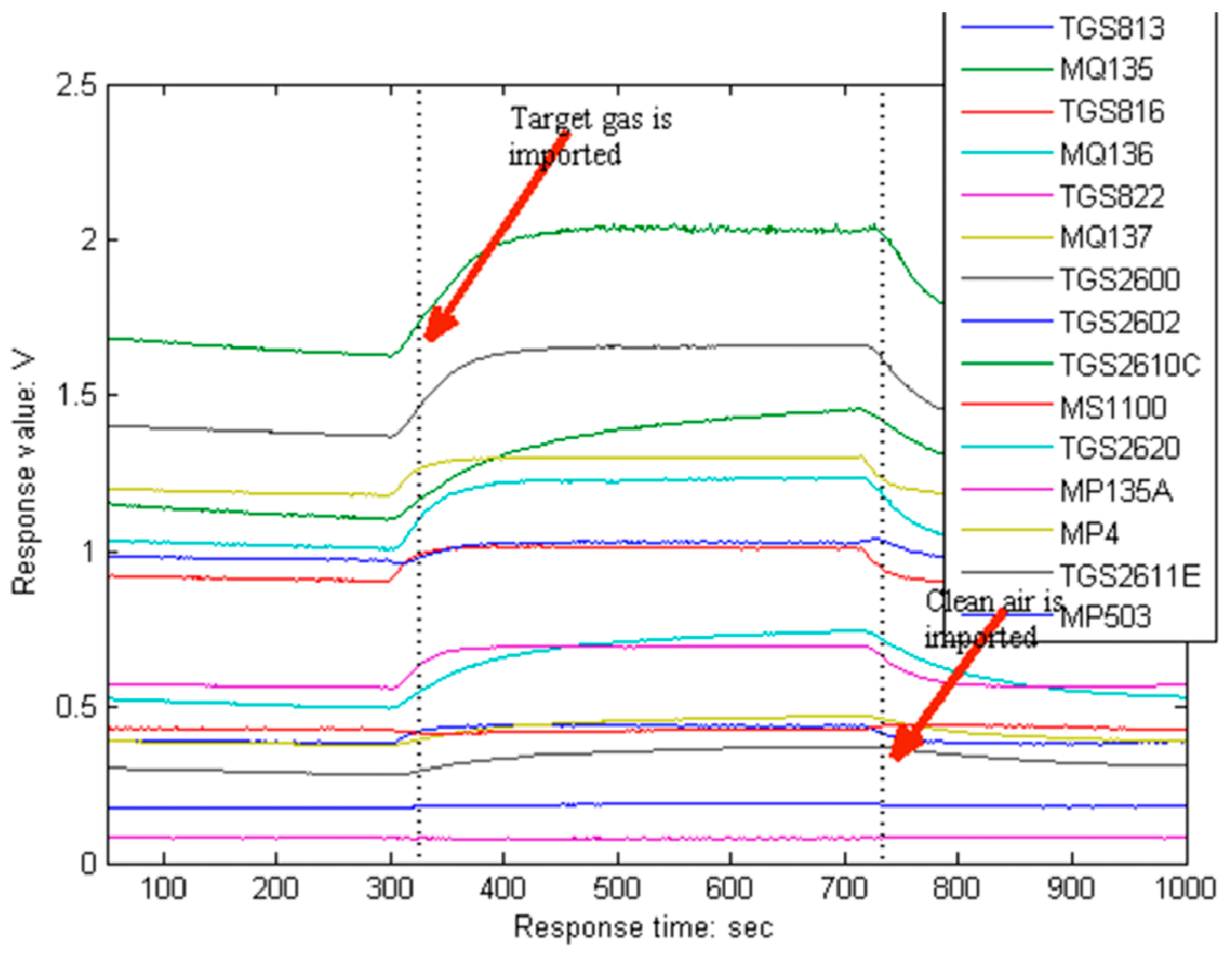
- Step (a)
- expose all sensors to clean air for 5 min to obtain the baseline.
- Step (b)
- introduce the target gas into the chamber for 7 min.
- Step (c)
- exposed the sensor array to clean air for 5 min again to clean the sensors and restore the baseline.
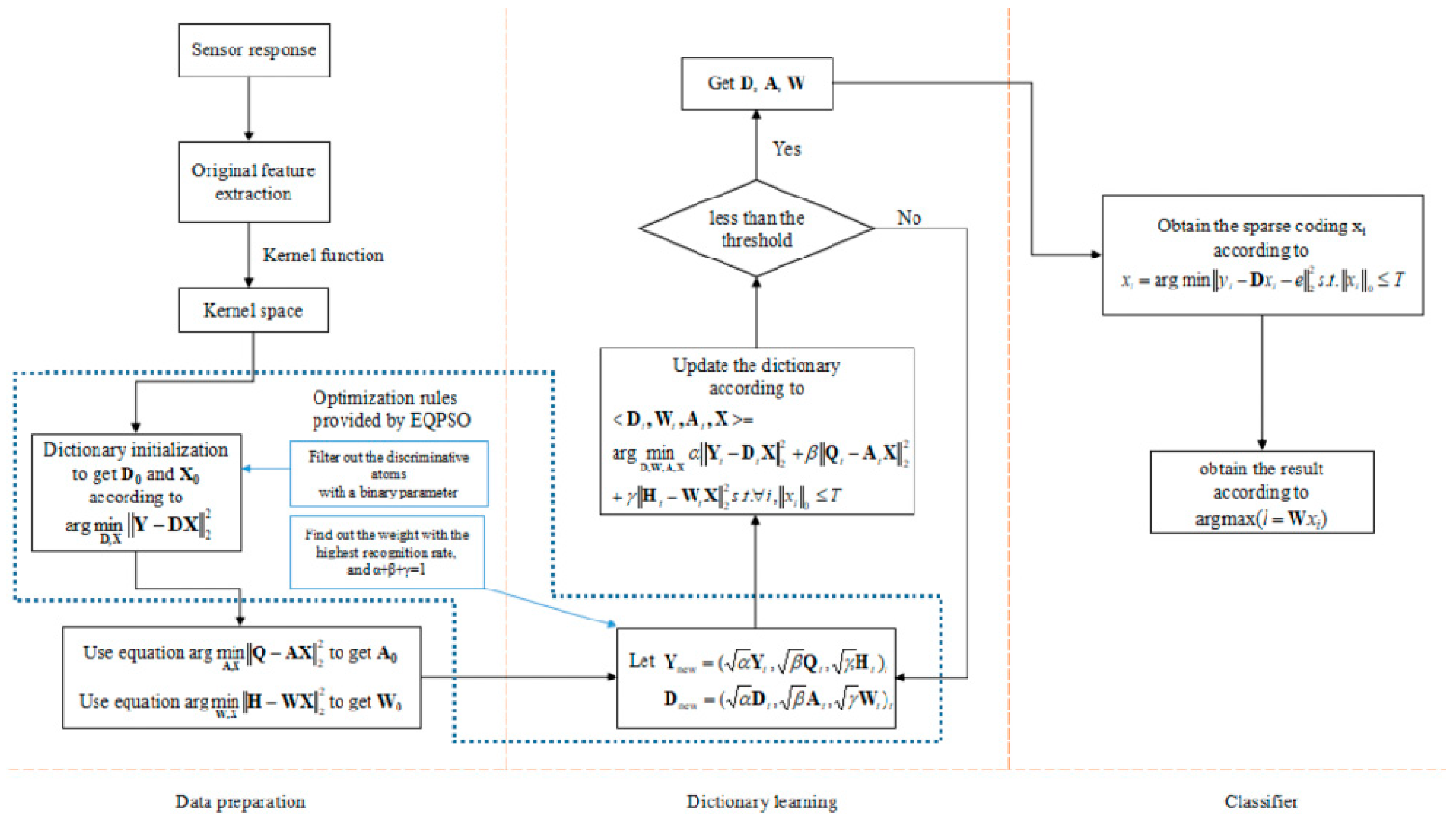
3. Methodology
3.1. KSVD and L-KSVD
3.2. Kernel Function
3.3. Dictionary
3.4. Weighted Coefficients
3.5. EQPSO and the Optimization Problem of the Proposed E-LCKSVD
3.5.1. PSO, QPSO and EQPSO
3.5.2. Optimization Problem of the Proposed E-LCKSVD
4. Results and Discussion
5. Conclusions
Author Contributions
Funding
Conflicts of Interest
References
- Högnadóttir, A.; Rouseff, R. Identification of aroma active compounds in orange essence oil using gas chromatography-olfactometry and gas chromatography-mass spectrometry. J. Chromatogr. A 2003, 998, 201–211. [Google Scholar] [CrossRef]
- Biniecka, M.; Caroli, S. Analytical methods for the quantification of volatile aromatic compounds. Trends Anal. Chem. 2011, 30, 1756–1770. [Google Scholar] [CrossRef]
- Pearce, T. Computational parallels between the biological olfactory pathway and its analogue ‘The Electronic Nose’: Part II. Sensor-based machine olfaction. Biosystems 1997, 41, 69–90. [Google Scholar] [CrossRef]
- Bahraminejad, B.; Basri, S.; Isa, M.; Hambali, Z. Application of a sensor array based on capillary-attached conductive gas sensors for odor identification. Meas. Sci. Technol. 2010, 21, 085204. [Google Scholar] [CrossRef]
- Jia, P.; Tian, F.; He, Q.; Fan, S.; Liu, J.; Yang, S.X. Feature extraction of wound infection data for electronic nose based on a novel weighted KPCA. Sens. Actuators B Chem. 2014, 201, 555–566. [Google Scholar] [CrossRef]
- Markom, M.A.; MdShakaff, A.Y.; Adom, A.H.; Ahmad, M.N.; Hidayat, W.; Abdullah, A.H.; Fikri, N.A. Intelligent electronic nose system for basal stem rot disease detection. Comput. Electron. Agric. 2009, 66, 140–146. [Google Scholar] [CrossRef]
- Gobbi, E.; Falasconi, M.; Torelli, E.; Sberveglier, G. Electronic nose predicts high and low fumonisin contamination in maize culture. Food Res. Int. 2011, 44, 992–999. [Google Scholar] [CrossRef]
- Loutfi, A.; Coradeschi, S.; Mani, G.; Shankar, P.; Rayappan, J. Electronic noses for food quality: A review. J. Food Eng. 2015, 144, 103–111. [Google Scholar] [CrossRef]
- Peris, M.; Escudergilabert, L. A 21st century technique for food control: Electronic noses. Anal. Chim. Acta 2009, 638, 1–15. [Google Scholar] [CrossRef] [PubMed]
- Licen, S.; Barbieri, G.; Fabbris, A.; Briguglio, S.C.; Pillon, A.; Stel, F.; Barbieri, P. Odor Control Map: Self Organizing Map built from electronic nose signals and integrated by different instrumental and sensorial data to obtain an assessment tool for real environmental scenarios. Sens. Actuators B Chem. 2018, 263, 476–485. [Google Scholar] [CrossRef]
- Yang, L.; Guo, C.; Zhao, J.; Pan, Y. Research advance in explosive detection by electronic nose. J. Transducer Technol. 2005, 24, 1–3. [Google Scholar]
- Wilson, A. Diverse Applications of Electronic-Nose Technologies in Agriculture and Forestry. Sensors 2013, 13, 2295–2348. [Google Scholar] [CrossRef] [PubMed]
- Chen, J.; Sun, Y.; Shen, L. Reach and Application of Electronic Nose on Testing the Quality of Agriculture Products. Appl. Mech. Mater. 2015, 738–739, 116–124. [Google Scholar] [CrossRef]
- Tobitsuka, K. Aroma components of La France and comparison of aroma patterns of different pears. Nippon Nōgeikagaku Kaishi 2003, 77, 762–767. [Google Scholar] [CrossRef]
- Saevels, S.; Lammertyn, J.; Berna, A.Z.; Veraverbeke, E.A.; Natale, C.D.; Nicolai, B.M. Electronic nose as a non-destructive tool to evaluate the optimal harvest date of apples. Postharvest Biol. Technol. 2004, 31, 9–19. [Google Scholar] [CrossRef]
- Natale, C.; Macagnano, A.; Davide, F.; Amico, A.D.; Paolesse, R.; Boschi, T.; Faccio, M.; Ferric, G. An electronic nose for food analysis. Sens. Actuators B Chem. 1997, 44, 521–526. [Google Scholar] [CrossRef]
- Mastello, R.B.; Capobiango, M.; Chin, S.; Monteriro, M.; Marriott, P.J. Identification of odour-active compounds of pasteurised orange juice using multidimensional gas chromatography techniques. Food Res. Int. 2015, 75, 281–288. [Google Scholar] [CrossRef] [PubMed]
- Leem, C.; Dreyfus, S. A Neural Network Approach to Feature Extraction in Sensor Signal Processing for Manufacturing Automation. J. Intell. Mater. Syst. Struct. 1994, 5, 247–257. [Google Scholar] [CrossRef]
- Eldar, Y.; Kuppinger, P.; Bölcskei, H. Compressed Sensing of Block-Sparse Signals: Uncertainty Relations and Efficient Recovery. Mathematics 2009, 58, 3042–3054. [Google Scholar]
- Jolliffe, I.T. Principal Component Analysis. J. Mark. Res. 2002, 87, 513. [Google Scholar]
- Hyvärinen, A. Fast and robust fixed-point algorithms for independent component analysis. IEEE Trans. Neural Netw. 1999, 10, 626–634. [Google Scholar] [CrossRef] [PubMed]
- Romdhani, S.; Gong, S.; Psarrou, A. A multi-view nonlinear active shape model using kernel PCA. Proc. BMVC 1999, 10, 483–492. [Google Scholar]
- Martin, Y.G.; Pavon, J.L.P.; Cordero, B.M.; Pinto, C.G. Classification of vegetable oils by linear discriminant analysis of electronic nose data. Anal. Chim. Acta 1999, 384, 83–94. [Google Scholar] [CrossRef]
- Saraoğlu, H.M.; Selvi, A.O.; Ebeoğlu, M.A.; Tasaltin, C. Electronic nose system based on quartz crystal microbalance sensor for blood glucose and hbA1c levels from exhaled breath odor. IEEE Sens. J. 2013, 13, 4229–4235. [Google Scholar] [CrossRef]
- Brudzewski, K.; Osowski, S.; Markiewicz, T. Classification of milk by means of an electronic nose and SVM neural network. Sens. Actuators B Chem. 2004, 98, 291–298. [Google Scholar] [CrossRef]
- Ahron, M.; Elad, M.; Bruckstein, A. K-SVD: An Algorithm for Designing Overcomplete Dictionaries for Sparse Representation. IEEE Trans. Image Process. 2006, 15, 4311–4322. [Google Scholar] [CrossRef]
- Marsousi, M.; Abhari, K.; Babyn, P.; Alirezaie, J. MULTI-STAGE OMP sparse coding using local matching pursuit atoms selection. IEEE Int. Conf. Acoust. 2013, 32, 1783–1787. [Google Scholar]
- Mairal, J.; Bach, F.; Ponce, J.; Sapiro, G. Online dictionary learning for sparse coding. In Proceedings of the 26th Annual International Conference on Machine Learning, Montreal, QC, Canada, 14–18 June 2009; pp. 689–696. [Google Scholar]
- Yang, M.; Dai, D.; Shen, L.; Gool, L. Latent Dictionary Learning for Sparse Representation Based Classification. In Proceedings of the IEEE Conference on Computer Vision and Pattern Recognition, Columbus, OH, USA, 23–28 June 2014; pp. 4138–4145. [Google Scholar]
- Thiagarajan, J.; Ramamurthy, K.; Spanias, A. Learning Stable Multilevel Dictionaries for Sparse Representation of Images. IEEE Trans. Neural Netw. Learn. Syst. 2013, 26, 1913–1926. [Google Scholar] [CrossRef] [PubMed]
- Fagin, R.; Halpern, J.; Moses, Y.; Vardi, M. Reasoning about Knowledge; MIT Press: Cambridge, MA, USA, 2003; Volume 67, pp. 503–525. [Google Scholar]
- Kennedy, J.; Eberhart, R. Particle swarm optimization. Icnn95-Int. Conf. Neural Netw. 2002, 4, 1942–1948. [Google Scholar]
- Zhou, H.; Wang, G. A new theory consistency index based on deduction theorems in several logic systems. Fuzzy Sets Syst. 2006, 157, 427–443. [Google Scholar] [CrossRef]
- Jia, P.; Duan, S.; Yan, J. An Enhanced Quantum-Behaved Particle Swarm Optimization Based on a Novel Computing Way of Local Attractor. Information 2015, 6, 633–649. [Google Scholar] [CrossRef]
- Jia, P.; Tian, F.; Fan, S.; He, Q.; Feng, J.; Yang, S.X. A novel sensor array and classifier optimization method of electronic nose based on enhanced quantum-behaved particle swarm optimization. Sens. Rev. 2014, 34, 304–311. [Google Scholar] [CrossRef]
- Huang, G.B.; Zhu, Q.Y.; Siew, C.K. Extreme learning machine: A new learning scheme of feedforward neural networks. IEEE Int. Jt. Conf. Neural Netw. 2004, 2, 985–990. [Google Scholar]


| No. | Compound | No. | Compound |
|---|---|---|---|
| 1 | Ethanal (C2H4O) | 26 | α-copaene (C15H24) |
| 2 | Ethyl acetate (C4H8O2) | 27 | Decanal (C10H20O) |
| 3 | Methyl butanoate (C5H10O2) | 28 | Linalool (C10H18O) |
| 4 | α-pinene (C10H16) | 29 | Germacrene D (C15H24) |
| 5 | α-thujene (C10H16) | 30 | Caryophyllene (C15H24) |
| 6 | Ethyl butanoate (C6H12O2) | 31 | P-menth-1-en-4-ol (C10H18O) |
| 7 | Butanoic acid,2-methyl-,ethyl ester (C7H14O2) | 32 | Citronellol acetate (C12H22O2) |
| 8 | Hexanal (C6H12O) | 33 | β-farnesene (C15H24) |
| 9 | β-pinene (C10H16) | 34 | p-menth-1-en-8-ol (C12H20O2) |
| 10 | β-thujene (C10H16) | 35 | Valencene (C15H24) |
| 11 | 3-carene (C10H16) | 36 | Nerol acetate (C12H20O2) |
| 12 | α-phellandrene (C10H16) | 37 | (S)-carvone (C10H14O) |
| 13 | β-myrcene (C10H16) | 38 | 1,6-octadiene,3-(1-ethoxyethoxy)-3, 7-dimethyl (C14H26O2) |
| 14 | α-terpinene (C10H16) | 39 | Cadinene (C15H24) |
| 15 | Limonene (C10H16) | 40 | Lavandulol acetate (C12H20O2) |
| 16 | β-phellandrene (C10H16) | 41 | 1-cyclohexene-1-methanol,4-(1-methylethenyl)-,acetate (C12H18O2) |
| 17 | Ethyl caproate (C8H16O2) | 42 | 1-octanol (C8H18O) |
| 18 | γ-terpinene (C10H16) | 43 | Cyclopentanecarboxylic acid,2-ethylcyclohexyl ester(C14H24O2) |
| 19 | β-ocimene (C10H16) | 44 | 2,2,3,5,6-pentamethyl-3-heptene (C12H24) |
| 20 | β-cymene (C10H14) | 45 | α-caryophyllene (C15H24) |
| 21 | Terpinolene (C10H16) | 46 | 1-undecanol (C11H24O) |
| 22 | Cyclopentanone,2-methyl (C6H10O) | 47 | 1-propene 3-(2 cyclopentenyl)-2-methyl-1 (C21H22) |
| 23 | Octanal (C8H16O) | 48 | Dimethyl phthalate (C10H10O4) |
| 24 | Nonanal (C9H18O) | 49 | 2,4-diphenyl-4-methyl-1-pentene (C18H20) |
| 25 | Octyl acetate(C10H20O2) | 50 | 2,4-diphenyl-4-methyl-2-pentene (C18H20) |
| Sensors | Sensitive Characteristics |
|---|---|
| TGS813 | Methane, Propane, Ethanol, Isobutane, Hydrogen, Carbon monoxide |
| TGS816 | Combustible gases, Methane, Propane, Butane, Carbon monoxide, Hydrogen, Ethanol, Isobutane |
| TGS822 | Organic solvent vapors, Methane, Carbon monoxide, Isobutane, n-Hexane, Benzene, Ethanol, Acetone |
| TGS2600 | Gaseous air contaminants, Methane, Carbon monoxide, Isobutane, Ethanol, Hydrogen |
| TGS2602 | VOCs, Odorous gases, Ammonia, Hydrogen sulfide, Toluene, Ethanol |
| TGS2610C | Ethanol, Methane, Propane, Combustible gases, Isobutane |
| TGS2611E | Methane, Propane, Isobutane |
| TGS2620 | Vapors of organic solvents, Combustible gases, Methane, Carbon monoxide, Isobutane, Hydrogen, Ethanol |
| MQ135A | Hydrogen, Smoke, Carbon monoxide, Ethanol |
| MQ135 | Ammonia, Benzene series material, Acetone, Carbon monoxide, Ethanol, Smoke |
| MQ136 | Hydrogen sulfide, Sulfur dioxide |
| MQ137 | Ammonia, Trimethylamine, Ethanolamine |
| MS1100 | Formaldehyde, Benzene, Toluene, Xylene, Aromatic compound |
| MP4 | Methane, Combustible gases, Biogas, Natural gas |
| MP503 | Smoke, Isobutane, Formaldehyde, Ethanol |
| No. | α | β | γ | Acc_Train (%) | Acc_Test (%) |
|---|---|---|---|---|---|
| 1 | 0.6 | 0.3 | 0.1 | 92.2 | 87.5 |
| 2 | 0.3 | 0.6 | 0.1 | 89.1 | 84.4 |
| 3 | 0.1 | 0.3 | 0.6 | 84.4 | 75.0 |
| 4 | 0.33 | 0.33 | 0.33 | 90.6 | 84.4 |
| 1. Weighted Coefficient | 2. Binary Number for Dictionary Initialization |
|---|---|
α + β + γ = 1, and | , The value of is 0 or 1. |
| Original Data | Kernel Data | |||
|---|---|---|---|---|
| KSVD+ELM | L-KSVD | K-KSVD+ELM | E-LCKSVD | |
| Acc_train | 76.9 | 84.4 | 88.9 | 93.8 |
| Acc_test | 76.0 | 81.3 | 81.3 | 87.5 |
| Sensors | Binary Number | |||||||||
|---|---|---|---|---|---|---|---|---|---|---|
| 1 | TGS813 | 1 | 0 | 0 | 1 | 1 | 1 | 1 | 1 | 0 |
| 2 | TGS816 | 1 | 1 | 0 | 1 | 1 | 1 | 1 | 0 | 1 |
| 3 | TGS822 | 1 | 0 | 1 | 1 | 1 | 0 | 1 | 1 | 0 |
| 4 | TGS2600 | 1 | 1 | 1 | 0 | 0 | 1 | 0 | 1 | 1 |
| 5 | TGS2602 | 1 | 0 | 1 | 1 | 1 | 1 | 0 | 1 | 1 |
| 6 | TGS2610C | 1 | 1 | 1 | 1 | 0 | 0 | 1 | 1 | 1 |
| 7 | TGS2611E | 1 | 0 | 1 | 0 | 1 | 1 | 0 | 1 | 1 |
| 8 | TGS2620 | 0 | 1 | 0 | 1 | 0 | 1 | 0 | 0 | 1 |
| 9 | MQ135A | 1 | 0 | 0 | 0 | 1 | 1 | 1 | 1 | 1 |
| 10 | MQ135 | 1 | 1 | 0 | 0 | 1 | 1 | 1 | 1 | 1 |
| 11 | MQ136 | 0 | 1 | 1 | 0 | 1 | 1 | 1 | 1 | 0 |
| 12 | MQ137 | 0 | 1 | 1 | 1 | 0 | 1 | 1 | 0 | 0 |
| 13 | MS1100 | 0 | 1 | 1 | 1 | 1 | 0 | 0 | 0 | 0 |
| 14 | MP4 | 1 | 1 | 1 | 1 | 0 | 0 | 1 | 0 | 1 |
| 15 | MP503 | 0 | 1 | 1 | 1 | 1 | 0 | 1 | 1 | 1 |
| Acc_train (%) | 90.6 | 92.2 | 89.0 | 98.4 | 90.6 | 81.3 | 93.8 | 98.4 | 85.9 | |
| Acc_test (%) | 81.3 | 84.4 | 87.5 | 93.8 | 71.9 | 75.0 | 87.5 | 96.9 | 81.3 | |
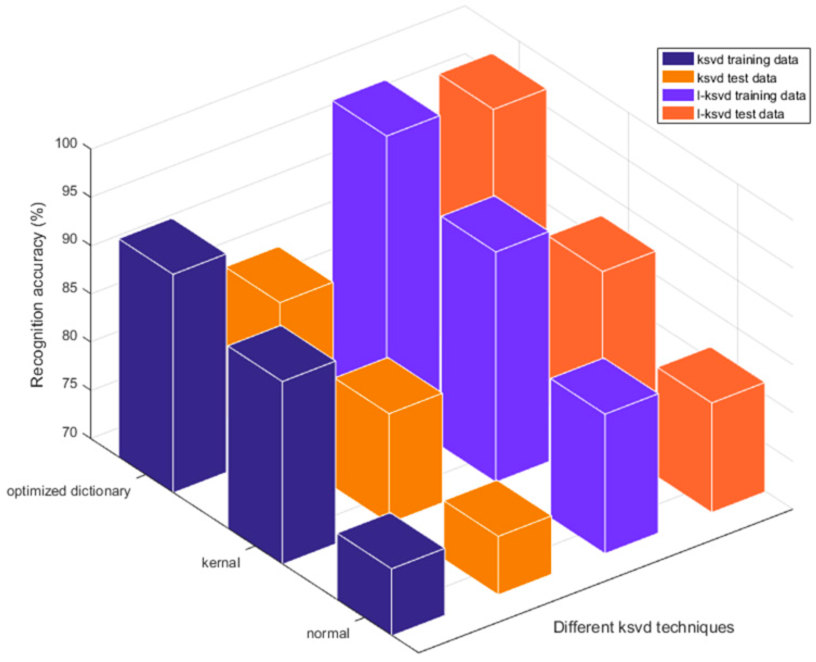
| Normal Dictionary Initialization | Optimized Dictionary Initialization | |||
|---|---|---|---|---|
| K-KSVD+ELM | E-LCKSVD | K-KSVD+ELM | E-LCKSVD | |
| Acc_train | 88.9 | 93.8 | 92.6 | 98.4 |
| Acc_test | 81.3 | 87.5 | 85.4 | 96.9 |
| No-Dealing | PCA | KPCA | ||
|---|---|---|---|---|
| SVM | Acc_train | 92.8 | 94.8 | 96.6 |
| Acc_test | 81.3 | 93.8 | 90.6 | |
| RBFNN | Acc_train | 89.5 | 91.0 | 94.8 |
| Acc_test | 86.5 | 88.5 | 89.6 | |
| K-LDA | Acc_train | 93.3 | 93.7 | 96.0 |
| Acc_test | 88.5 | 86.5 | 88.5 | |
| Advantages and Drawbacks | |
|---|---|
| PCA | This linear feature extraction algorithm obtains the new feature according to the variance contribution rate, but the effect is not satisfactory when dealing with the nonlinear data. |
| KPCA | With the help of the kernel function, the data can be mapped to a high-dimension space and then analyzed by PCA, which has the ability of processing the nonlinear data, but the high-dimension mapping increases the computational complexity. |
| K-LDA | LDA is a kind of supervised linear classifier. With the help of the kernel function, it has the ability to classify the nonlinear data to some extent, but the improvement of the recognition rate of the kernel function is limited. |
| RBFNN | An artificial neural network used in an E-nose earlier: using a radial basis function as the nonlinear mapping function, the recognition rate is better than K-LDA, but still lower than SVM. |
| SVM | For a long time, SVM is considered as an optimal classifier. With the help of the kernel function, SVM has an excellent ability to process data, but the recognition rate is affected by the quality of the input data. |
| E-LCKSVD | The feature extraction and classifier are integrated into one, considering the influence of the dictionary initialization, kernel function and weight coefficient of the objective function on the recognition rate; if the idea of semi-supervised learning can be added, it would be more valuable to use unlabeled data which is cheap and easily available. |
© 2019 by the authors. Licensee MDPI, Basel, Switzerland. This article is an open access article distributed under the terms and conditions of the Creative Commons Attribution (CC BY) license (http://creativecommons.org/licenses/by/4.0/).
Share and Cite
Cao, W.; Liu, C.; Jia, P. Feature Extraction and Classification of Citrus Juice by Using an Enhanced L-KSVD on Data Obtained from Electronic Nose. Sensors 2019, 19, 916. https://doi.org/10.3390/s19040916
Cao W, Liu C, Jia P. Feature Extraction and Classification of Citrus Juice by Using an Enhanced L-KSVD on Data Obtained from Electronic Nose. Sensors. 2019; 19(4):916. https://doi.org/10.3390/s19040916
Chicago/Turabian StyleCao, Wen, Chunmei Liu, and Pengfei Jia. 2019. "Feature Extraction and Classification of Citrus Juice by Using an Enhanced L-KSVD on Data Obtained from Electronic Nose" Sensors 19, no. 4: 916. https://doi.org/10.3390/s19040916
APA StyleCao, W., Liu, C., & Jia, P. (2019). Feature Extraction and Classification of Citrus Juice by Using an Enhanced L-KSVD on Data Obtained from Electronic Nose. Sensors, 19(4), 916. https://doi.org/10.3390/s19040916