Microfluidic Microwave Sensor for Detecting Saline in Biological Range


Abstract
:1. Introduction
2. Materials and Methods
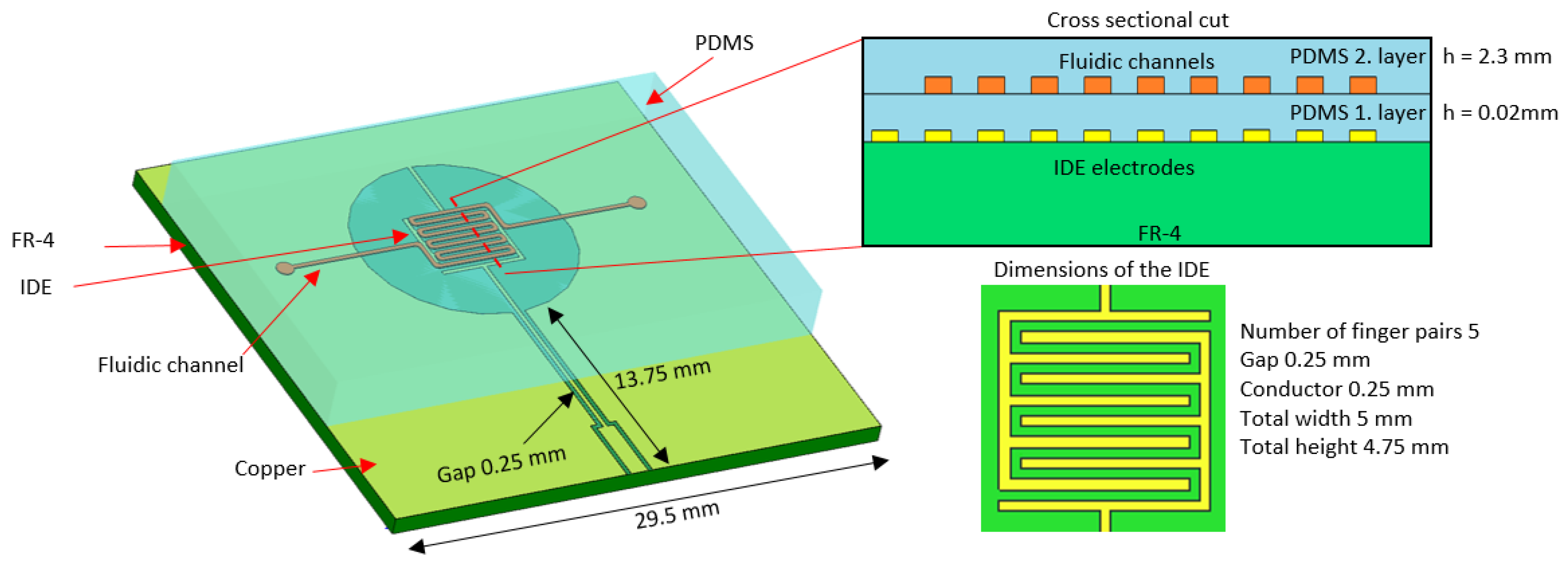
2.1. Sensor Design
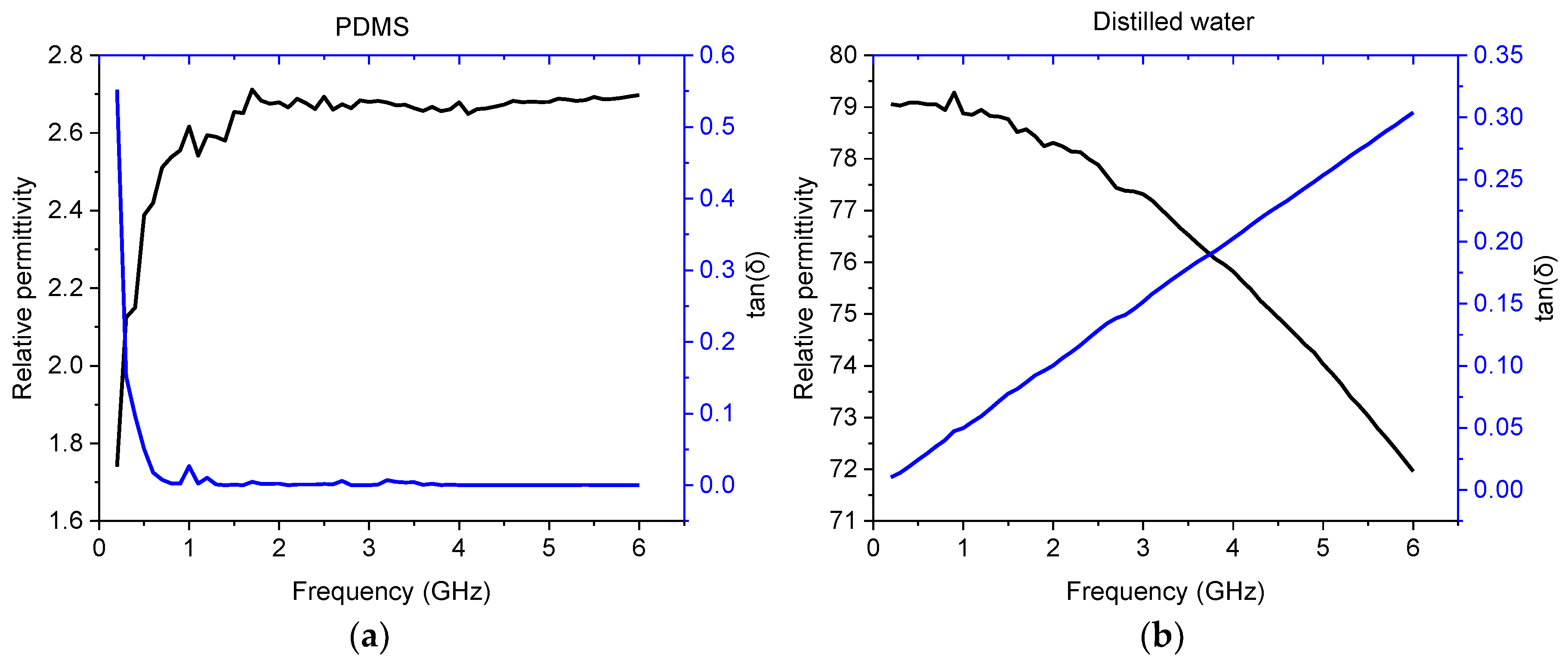
2.2. Modeling and Simulation
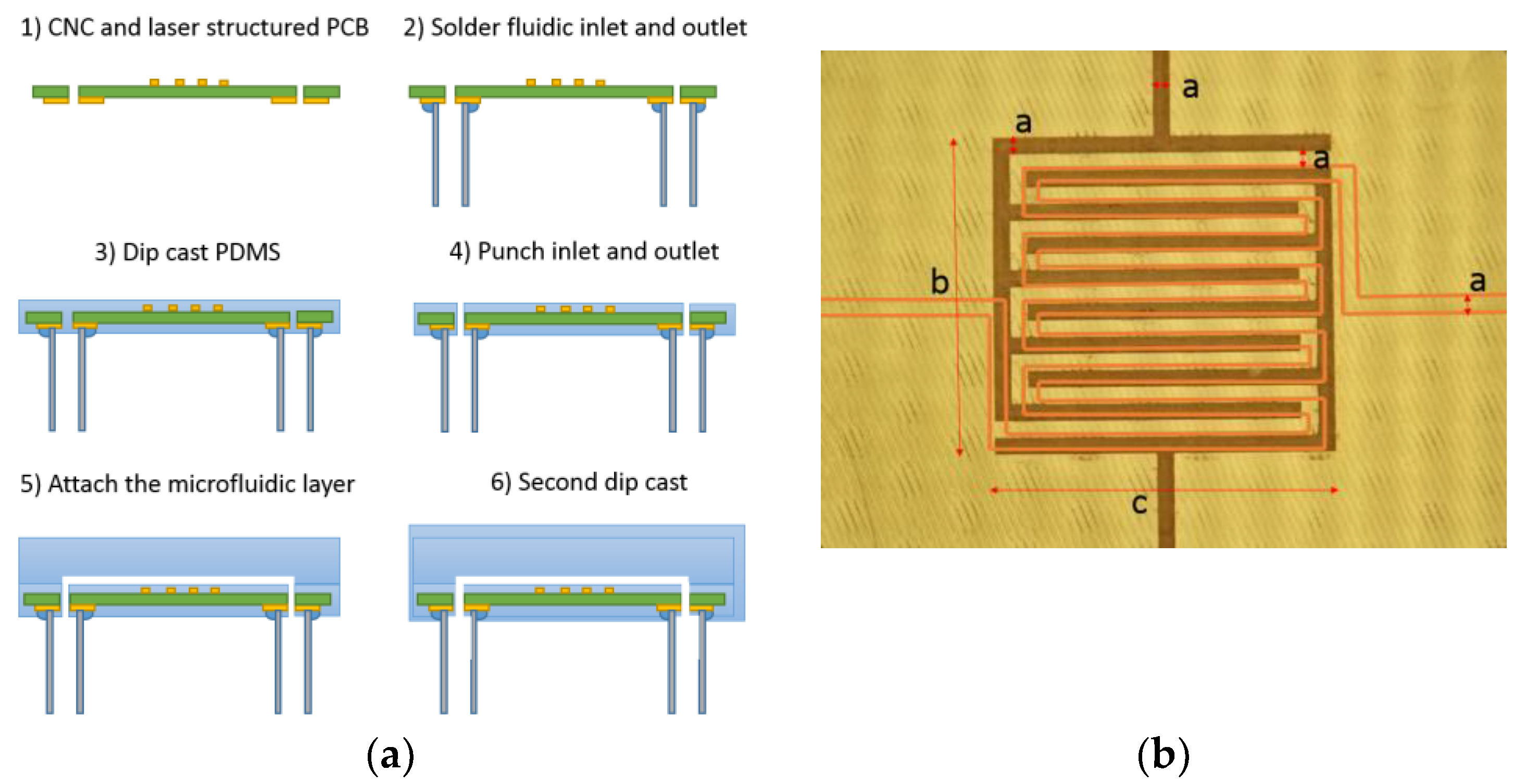
2.3. Manufacturing the Sensor and Microfluidics
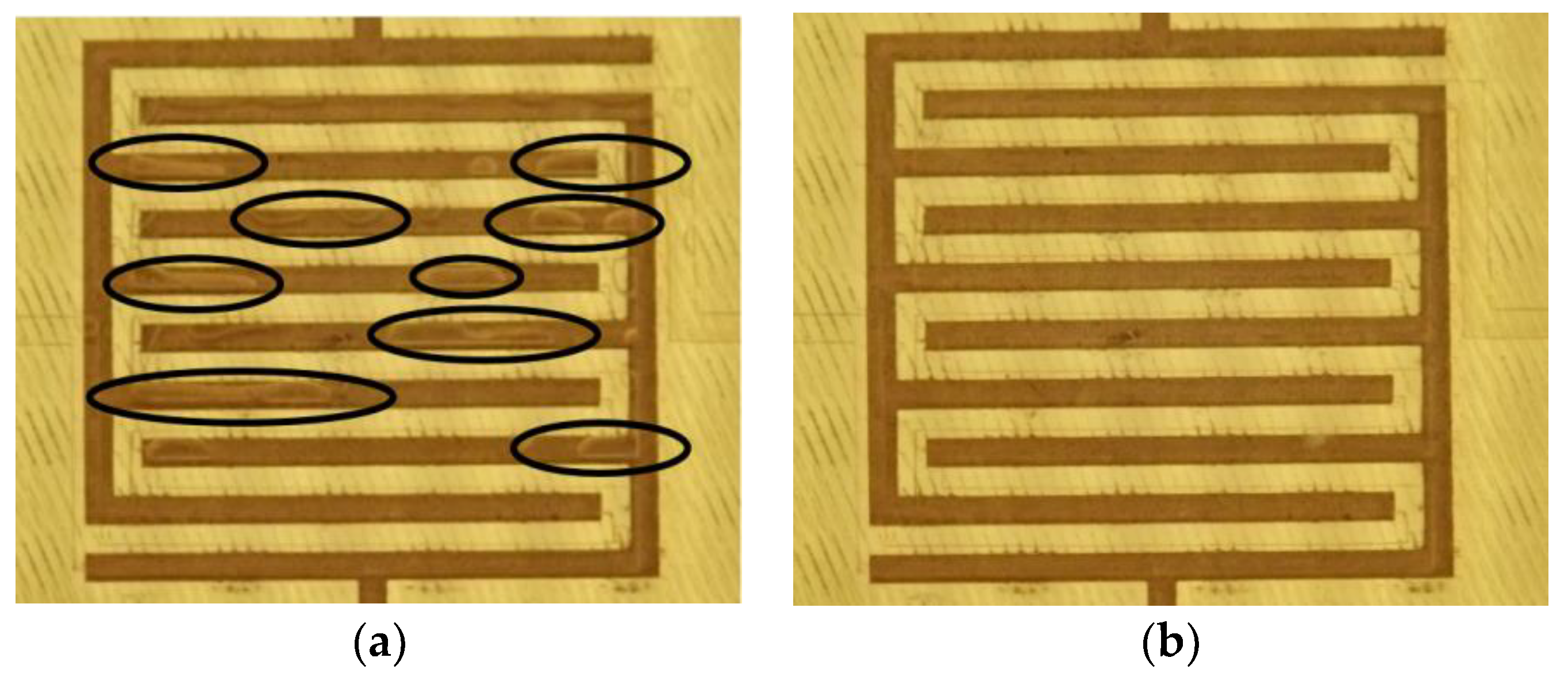
2.4. Sample Loading and Bubbles
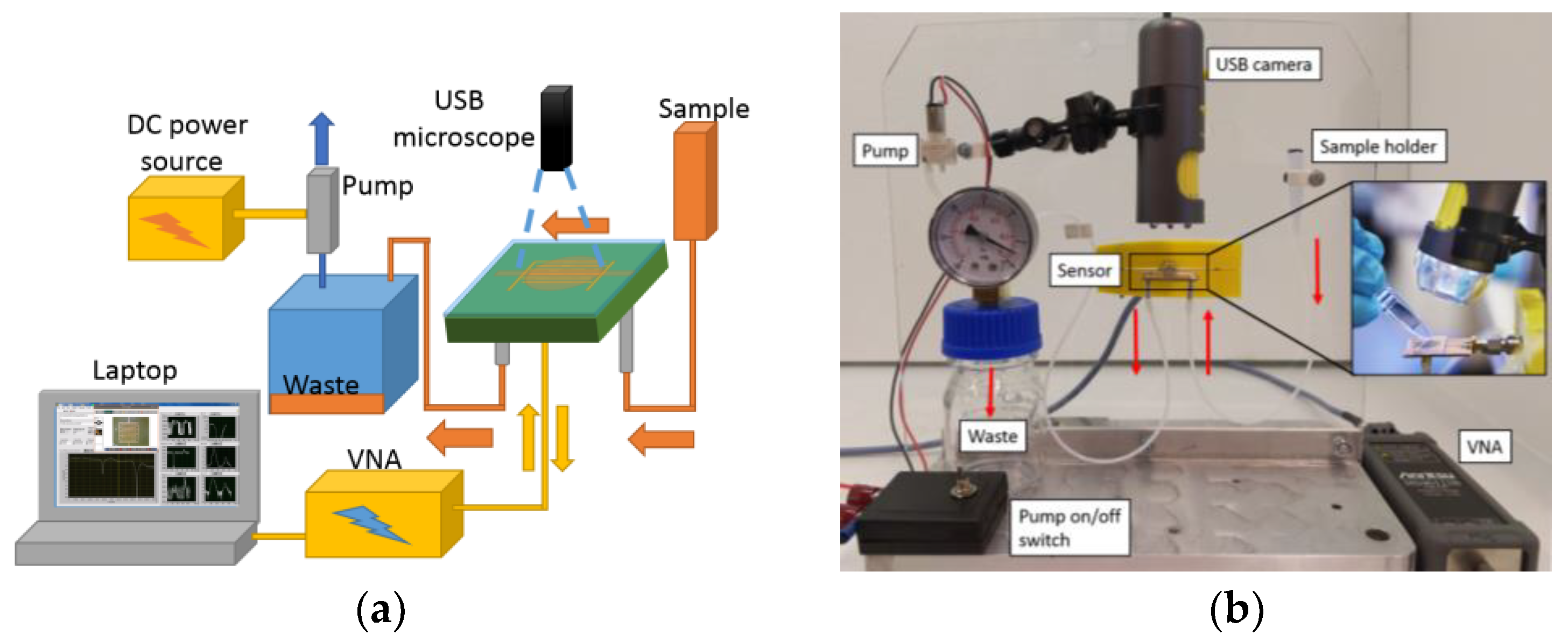
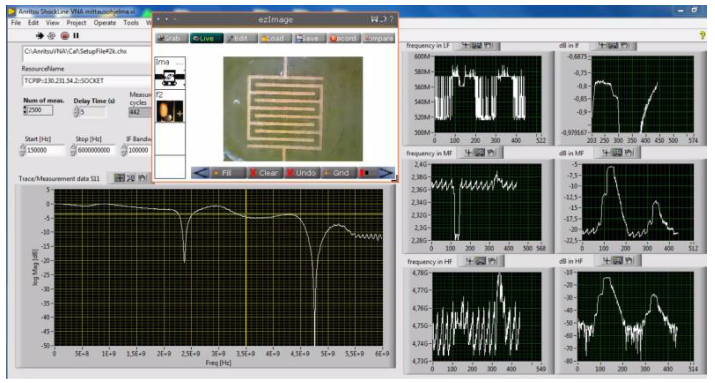
2.5. Measurement Method
2.6. Measured Samples
3. Results
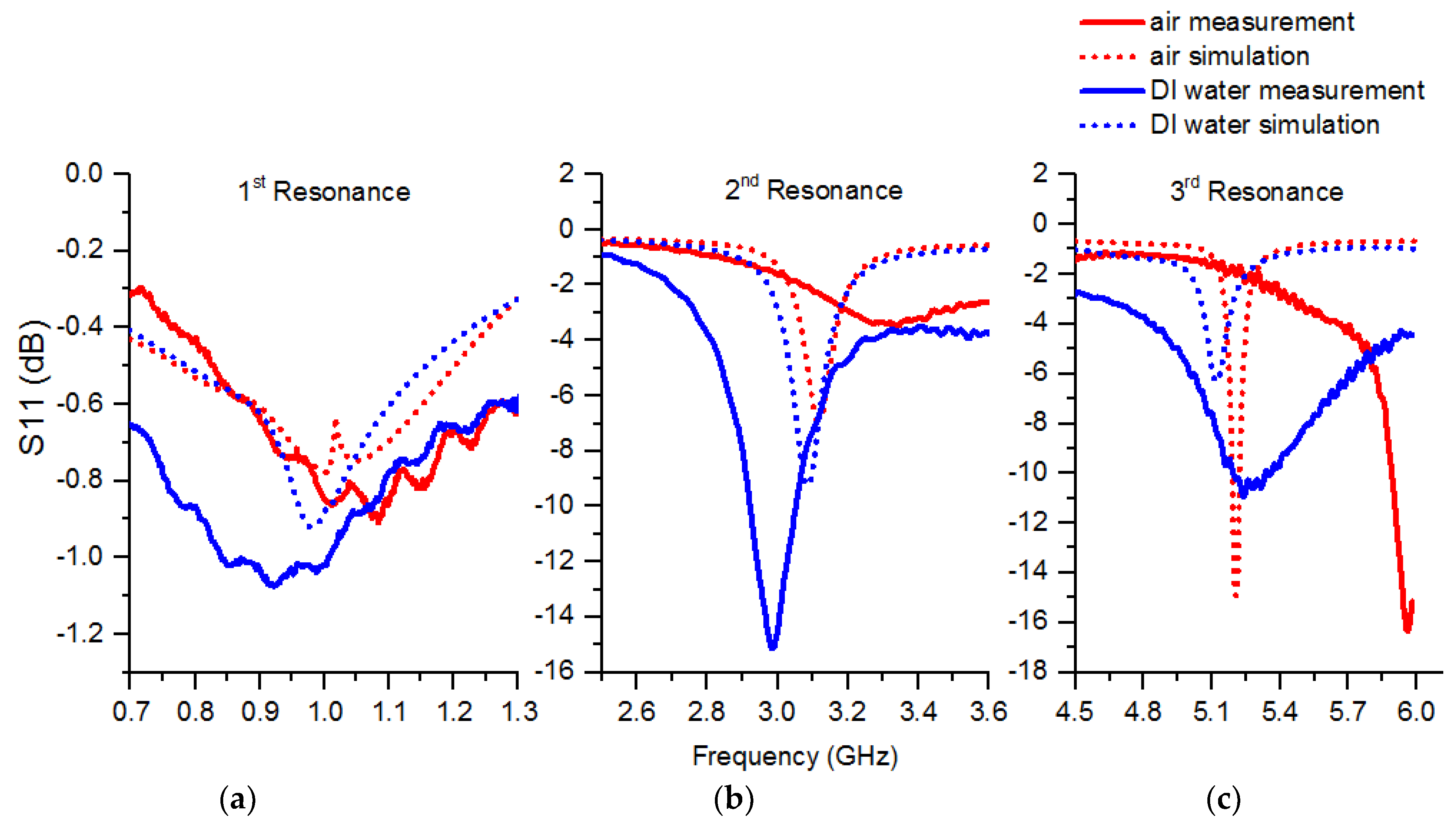
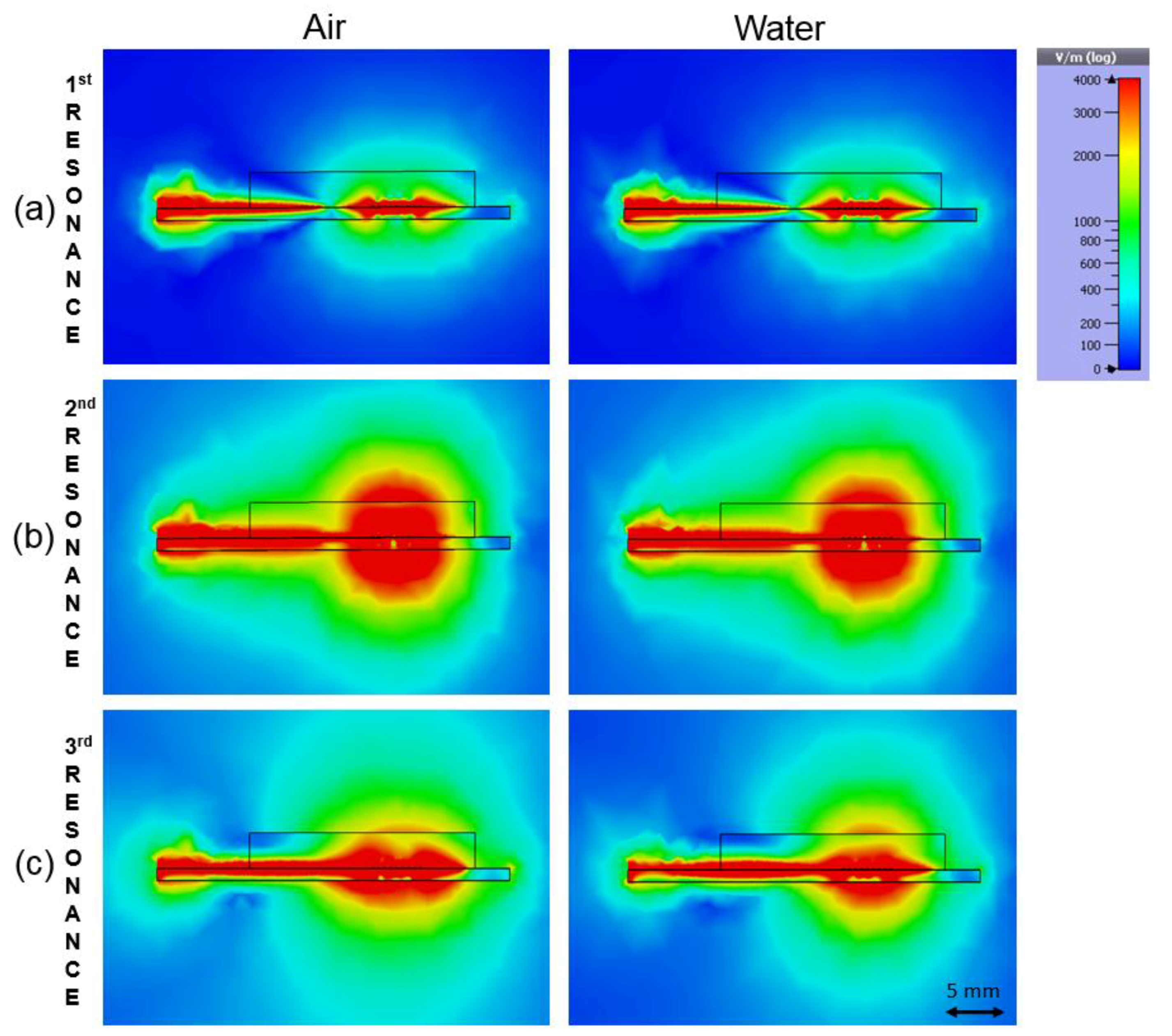
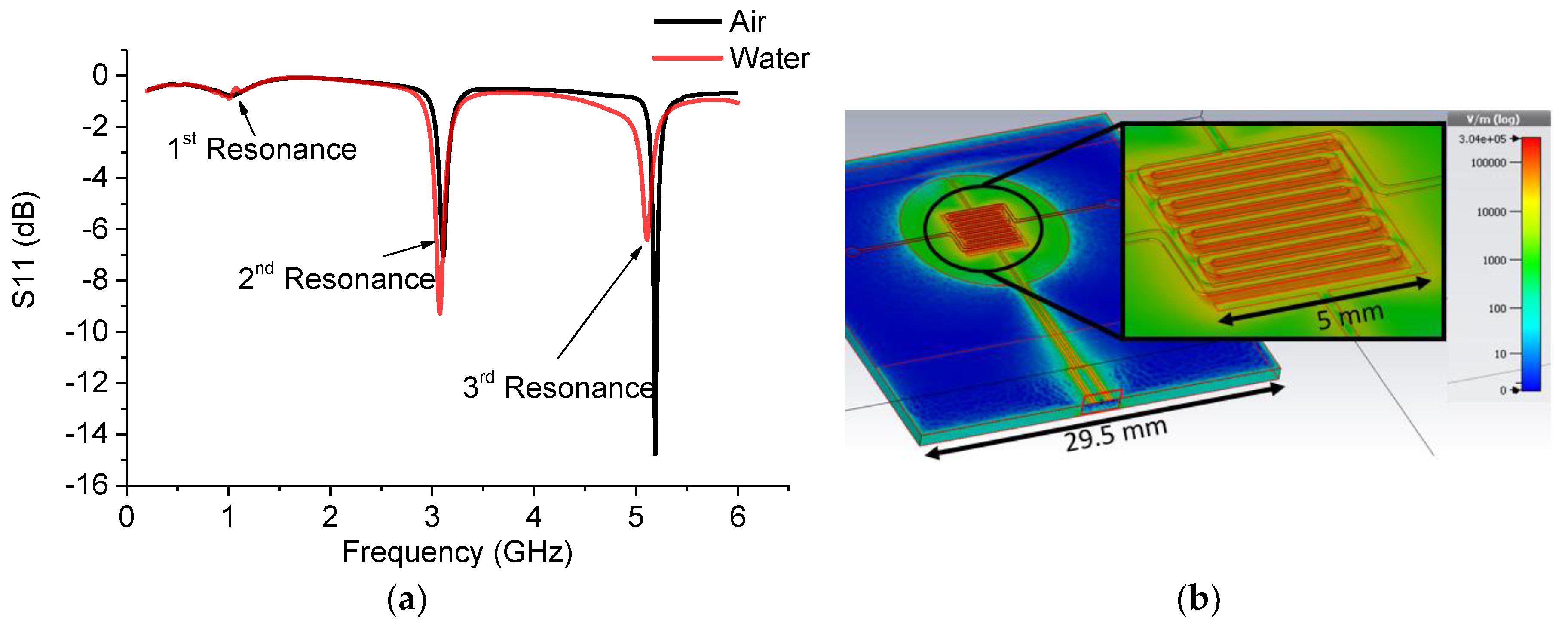
3.1. Simulation Results
3.2. Measurement Results
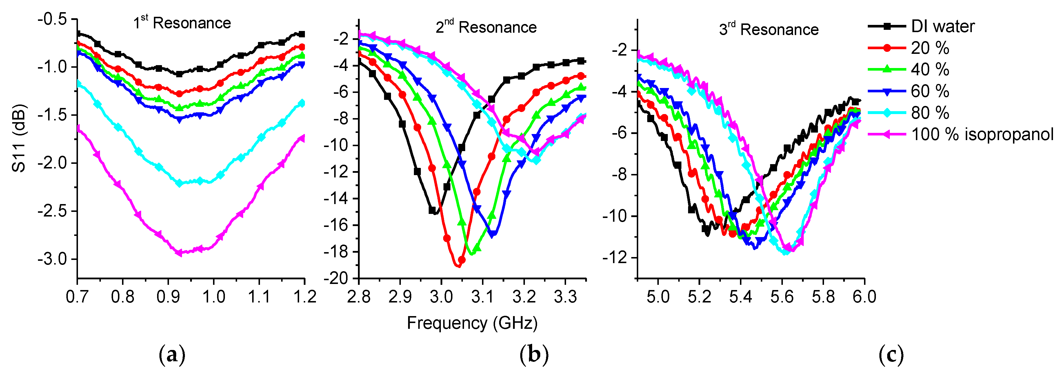
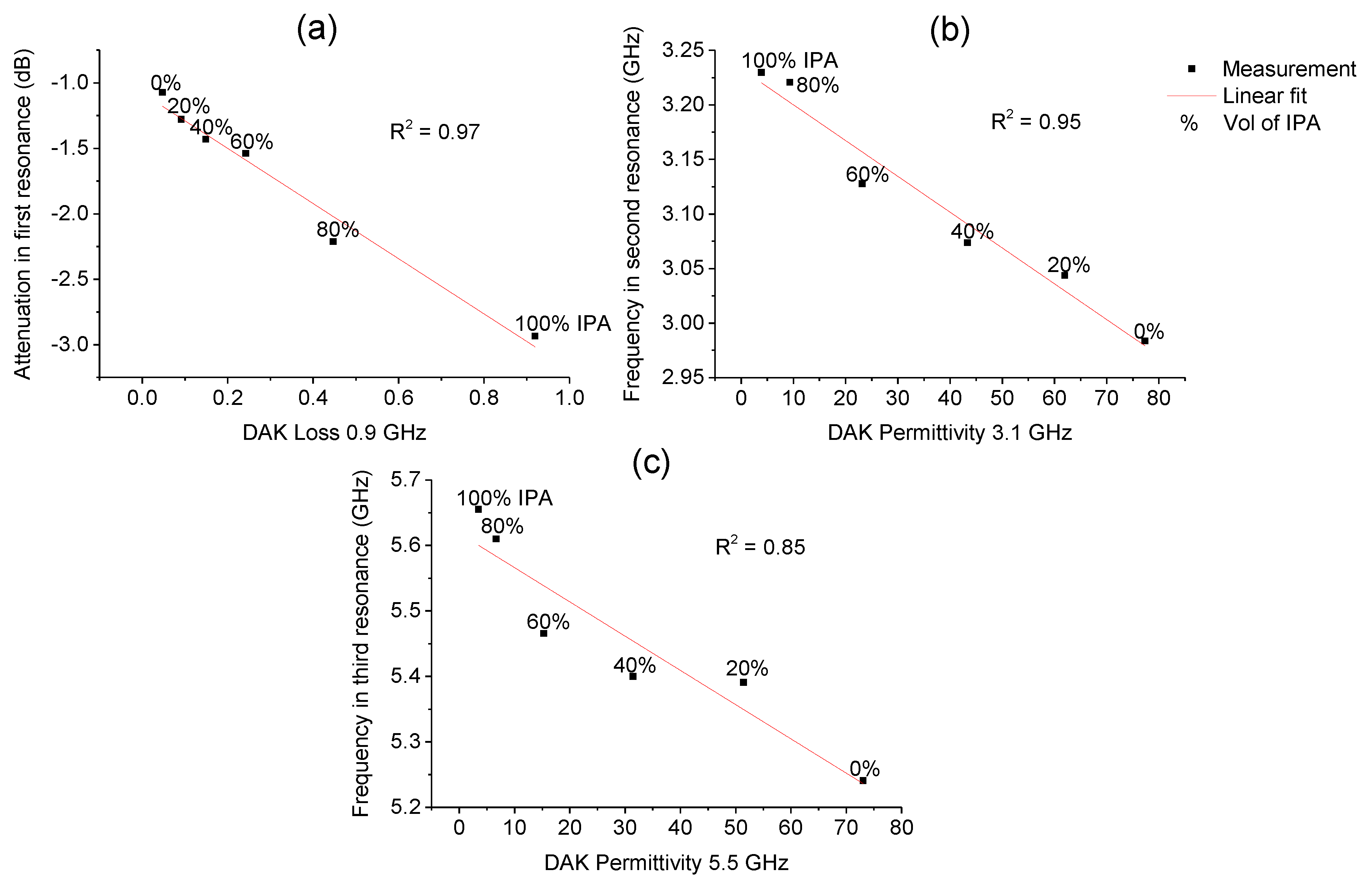
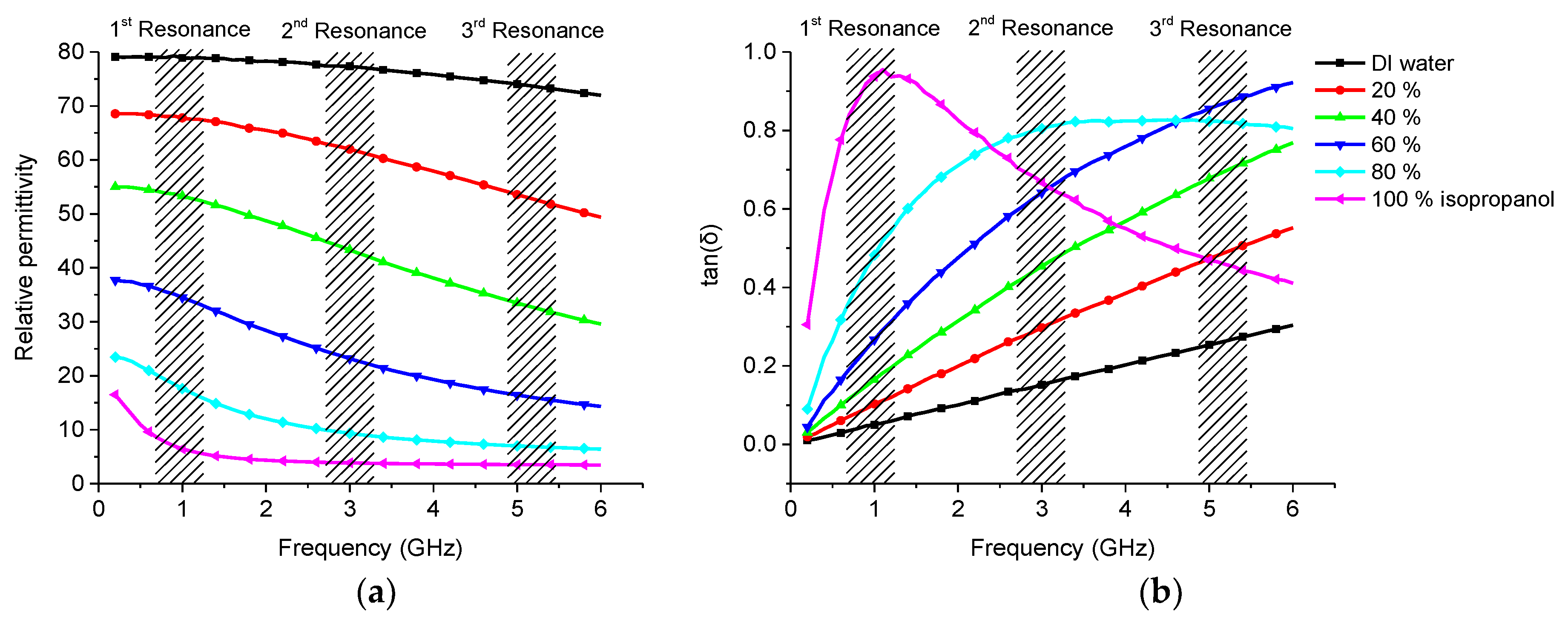
3.2.1. Isopropanol
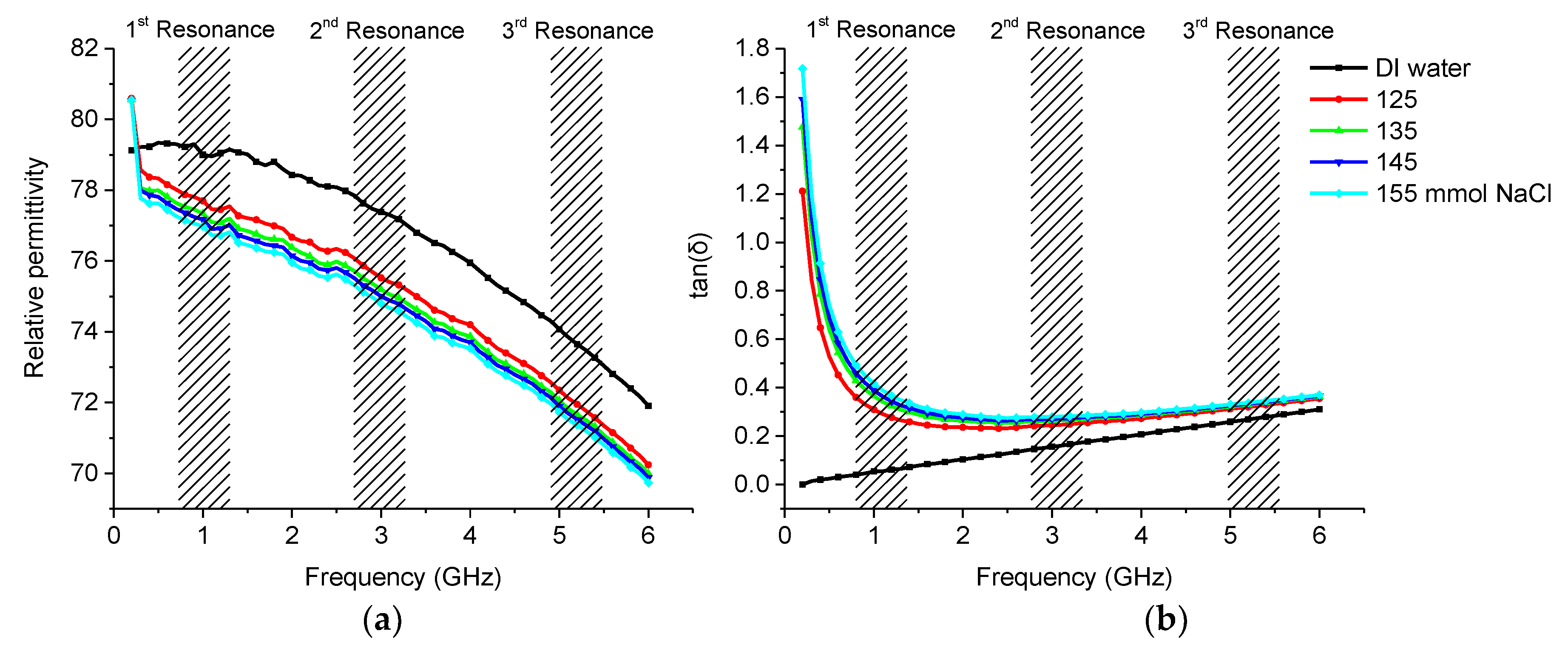
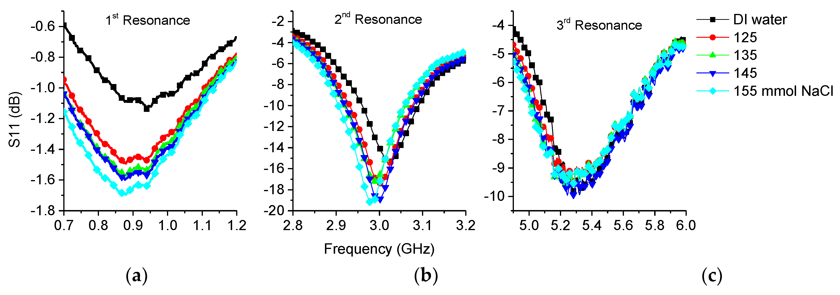
3.2.2. Saline
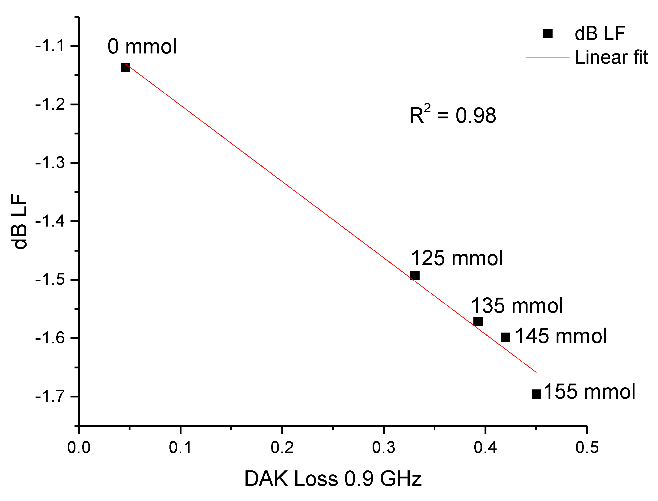
3.3. Sensor Performance
4. Discussion
5. Conclusions
Author Contributions
Funding
Acknowledgments
Conflicts of Interest
References
- Nyfors, E. Industrial Microwave Sensors—A Review. Subsurf. Sens. Technol. Appl. 2000, 1, 23–43. [Google Scholar] [CrossRef]
- Tinga, W.R.; Edwards, E.M. Dielectric Measurements Using Swept Frequency Techniques. J. Microw. Power 1968, 3, 114–125. [Google Scholar] [CrossRef]
- Stuchly, M.A.; Stuchly, M.A.; Stuchly, S.S. Coaxial Line Reflection Methods for Measuring Dielectric Properties of Biological Substances at Radio and Microwave Frequencies—A Review. IEEE Trans. Instrum. Meas. 1980, IM-29, 176–183. [Google Scholar] [CrossRef]
- Schmidt & Partner Engineering AG. Dielectric Assessment Kit. Available online: https://www.speag.com/products/dak/dielectric-measurements/ (accessed on 8 May 2018).
- Bao, X.; Ocket, I.; Crupi, G.; Schreurs, D.; Bao, J.; Kil, D.; Puers, B.; Nauwelaers, B. A Planar One-Port Microwave Microfluidic Sensor for Microliter Liquids Characterization. IEEE J. Electromagn. RF Microw. Med. Biol. 2018. [Google Scholar] [CrossRef]
- Gravesen, P.; Branebjerg, J.; Jensen, O.S. Microfluidics-a review. J. Micromech. Microeng. 1993, 3, 168–182. [Google Scholar] [CrossRef]
- Booth, J.C.; Orloff, N.D.; Mateu, J.; Janezic, M.; Rinehart, M.; Beall, J.A. Quantitative permittivity measurements of nanoliter Liquid volumes in microfluidic channels to 40 GHz. IEEE Trans. Instrum. Meas. 2010, 59, 3279–3288. [Google Scholar] [CrossRef]
- Sardi, G.M.; Lucibello, A.; Cursi, F.; Proietti, E.; Marcelli, R. A microfluidic sensor in coplanar waveguide configuration for localized micrometric liquid spectroscopy in microwaves regime. Microsyst. Technol. 2018, 1–11. [Google Scholar] [CrossRef]
- Salim, A.; Kim, S.H.; Park, J.Y.; Lim, S. Microfluidic Biosensor Based on Microwave Substrate-Integrated Waveguide Cavity Resonator. J. Sens. 2018, 2018. [Google Scholar] [CrossRef]
- Chen, T.; Dubuc, D.; Poupot, M.; Fournie, J.J.; Grenier, K. Accurate nanoliter liquid characterization up to 40 GHz for biomedical applications: Toward noninvasive living cells monitoring. IEEE Trans. Microw. Theory Tech. 2012, 60, 4171–4177. [Google Scholar] [CrossRef]
- Salim, A.; Lim, S. TM02quarter-mode substrate-integrated waveguide resonator for dual detection of chemicals. Sensors 2018, 18, 1964. [Google Scholar] [CrossRef]
- Naumova, N.; Hlukhova, H.; Barannik, A.; Gubin, A.; Protsenko, I.; Cherpak, N.; Vitusevich, S. Microwave characterization of low-molecular-weight antioxidant specific biomarkers. Biochim. Biophys. Acta-Gen. Subj. 2019, 1863, 226–231. [Google Scholar] [CrossRef]
- Hamzah, H.; Abduljabar, A.; Lees, J.; Porch, A. A compact microwave microfluidic sensor using a re-entrant cavity. Sensors 2018, 18, 910. [Google Scholar] [CrossRef] [PubMed]
- Liu, C.F.; Wang, M.H.; Jang, L.S. Microfluidics-based hairpin resonator biosensor for biological cell detection. Sensors Actuators B Chem. 2018, 263, 129–136. [Google Scholar] [CrossRef]
- Hamzah, H.; Lees, J.; Porch, A. Split ring resonator with optimised sensitivity for microfluidic sensing. Sens. Actuators A Phys. 2018, 276, 1–10. [Google Scholar] [CrossRef]
- Li, C.H.; Chen, K.W.; Yang, C.L.; Lin, C.H.; Hsieh, K.C. A urine testing chip based on the complementary split-ring resonator and microfluidic channel. In Proceedings of the IEEE International Conference on Micro Electro Mechanical Systems (MEMS), Belfast, UK, 21–25 January 2018; pp. 1150–1153. [Google Scholar]
- Zarifi, M.H.; Sadabadi, H.; Hejazi, S.H.; Daneshmand, M.; Sanati-Nezhad, A. Noncontact and Nonintrusive Microwave-Microfluidic Flow Sensor for Energy and Biomedical Engineering. Sci. Rep. 2018, 8. [Google Scholar] [CrossRef] [PubMed]
- Narang, R.; Mohammadi, S.; Ashani, M.M.; Sadabadi, H.; Hejazi, H.; Zarifi, M.H.; Sanati-Nezhad, A. Sensitive, Real-time and Non-Intrusive Detection of Concentration and Growth of Pathogenic Bacteria using Microfluidic-Microwave Ring Resonator Biosensor. Sci. Rep. 2018, 8. [Google Scholar] [CrossRef] [PubMed]
- Abduljabar, A.A.; Hamzah, H.; Porch, A. Double Microstrip Microfluidic Sensor for Temperature Correction of Liquid Characterization. IEEE Microw. Wirel. Compon. Lett. 2018, 28, 735–737. [Google Scholar] [CrossRef]
- Jilnai, M.T.; Wen, W.P.; Cheong, L.Y.; Rehman, M.Z.U. A microwave ring-resonator sensor for non-invasive assessment of meat aging. Sensors 2016, 16, 52. [Google Scholar] [CrossRef]
- Yesiloz, G.; Boybay, M.S.; Ren, C.L. Label-free high-throughput detection and content sensing of individual droplets in microfluidic systems. Lab Chip 2015, 15, 4008–4019. [Google Scholar] [CrossRef]
- Reynolds, R.M.; Padfield, P.L.; Seckl, J.R. Disorders Of Sodium Balance Clinical review Disorders of sodium balance Queen’s Medical Control of sodium balance. Source BMJ Br. Med. J. 2006, 332, 702–705. [Google Scholar] [CrossRef]
- Guo, J.; Li, C.M.; Kang, Y. PDMS-film coated on PCB for AC impedance sensing of biological cells. Biomed. Microdevices 2014, 16, 681–686. [Google Scholar] [CrossRef] [PubMed]
- Verbalis, J.G.; Goldsmith, S.R.; Greenberg, A.; Korzelius, C.; Schrier, R.W.; Sterns, R.H.; Thompson, C.J. Diagnosis, evaluation, and treatment of hyponatremia: Expert panel recommendations. Am. J. Med. 2013, 126. [Google Scholar] [CrossRef]
- Muhsin, S.A.; Mount, D.B. Diagnosis and treatment of hypernatremia. Best Pract. Res. Clin. Endocrinol. Metab. 2016, 30, 189–203. [Google Scholar] [CrossRef] [PubMed]
- Nyfors, E.; Vainikainen, P. Industrial Microwave Sensors; Artech House: Norwood, MA, USA, 1989. [Google Scholar]
- Nasr, I.; Nehring, J.; Aufinger, K.; Fischer, G.; Weigel, R.; Kissinger, D. Single-and dual-port 50-100-GHz integrated vector network analyzers with on-chip dielectric sensors. IEEE Trans. Microw. Theory Tech. 2014, 62, 2168–2179. [Google Scholar] [CrossRef]
- Chung, H.; Ma, Q.; Sayginer, M.; Rebeiz, G.M. A 0.01-26 GHz single-chip SiGe reflectometer for two-port vector network analyzers. In Proceedings of the 2017 IEEE MTT-S International Microwave Symposium Digest, Honololu, HI, USA, 4–9 June 2017; pp. 1259–1261. [Google Scholar]
- Nehring, J.; Schutz, M.; Dietz, M.; Nasr, I.; Aufinger, K.; Weigel, R.; Kissinger, D. Highly Integrated 4-32-GHz Two-Port Vector Network Analyzers for Instrumentation and Biomedical Applications. IEEE Trans. Microw. Theory Tech. 2017, 65, 229–244. [Google Scholar] [CrossRef]


| Sample | 1st Frequency/Attenuation GHz/dB | 2nd Frequency/Attenuation GHz/dB | 3rd Frequency/Attenuation GHz/dB |
|---|---|---|---|
| Air | 1.024/−0.785 | 3.106/−7.019 | 5.189/−14.777 |
| DI water | 1.006/−0.901 | 3.077/−9.285 | 5.113/−6.400 |
| Sample | 1st Resonance/Attenuation GHz/dB | 2nd Resonance/Attenuation GHz/dB | 3rd Resonance/Attenuation GHz/dB |
|---|---|---|---|
| Air measurement | 1.084/−0.908 | 3.341/−3.499 | 5.961/−16.359 |
| Air simulation | 1.006/−0.778 | 3.109/−6.859 | 5.189/−14.919 |
| Water measurement | 0.922/−1.074 | 2.984/−15.140 | 5.241/−10.937 |
| Water simulation | 0.983/−0.921 | 3.077/−9.224 | 5.107/−6.318 |
| Air-water measurement | Δ(−0.162/−0.166) | Δ(−0.357/−11.641) | Δ(−0.720/+5.422) |
| Air-water simulation | Δ(−0.023/−0.143) | Δ(−0.032/-2.365) | Δ(−0.082/+8.601) |
© 2019 by the authors. Licensee MDPI, Basel, Switzerland. This article is an open access article distributed under the terms and conditions of the Creative Commons Attribution (CC BY) license (http://creativecommons.org/licenses/by/4.0/).
Share and Cite
Kilpijärvi, J.; Halonen, N.; Juuti, J.; Hannu, J. Microfluidic Microwave Sensor for Detecting Saline in Biological Range. Sensors 2019, 19, 819. https://doi.org/10.3390/s19040819
Kilpijärvi J, Halonen N, Juuti J, Hannu J. Microfluidic Microwave Sensor for Detecting Saline in Biological Range. Sensors. 2019; 19(4):819. https://doi.org/10.3390/s19040819
Chicago/Turabian StyleKilpijärvi, Joni, Niina Halonen, Jari Juuti, and Jari Hannu. 2019. "Microfluidic Microwave Sensor for Detecting Saline in Biological Range" Sensors 19, no. 4: 819. https://doi.org/10.3390/s19040819
APA StyleKilpijärvi, J., Halonen, N., Juuti, J., & Hannu, J. (2019). Microfluidic Microwave Sensor for Detecting Saline in Biological Range. Sensors, 19(4), 819. https://doi.org/10.3390/s19040819