A Novel Surface Descriptor for Automated 3-D Object Recognition and Localization


Abstract
:
1. Introduction
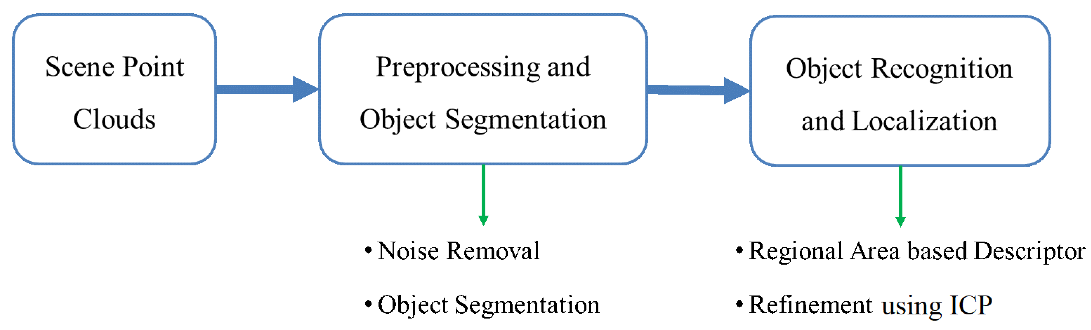
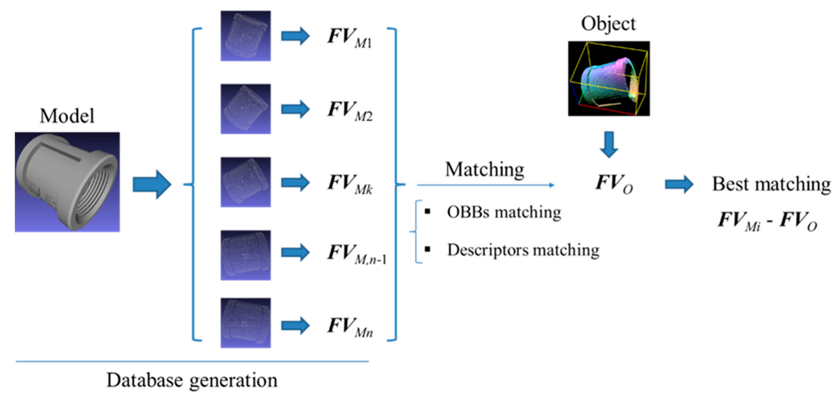
2. Methodology
| Algorithm 1: |
| Input: Measured point cloud O and model point cloud M. |
| Output: Position and Orientation of objects. |
|
2.1. Object Segmentation
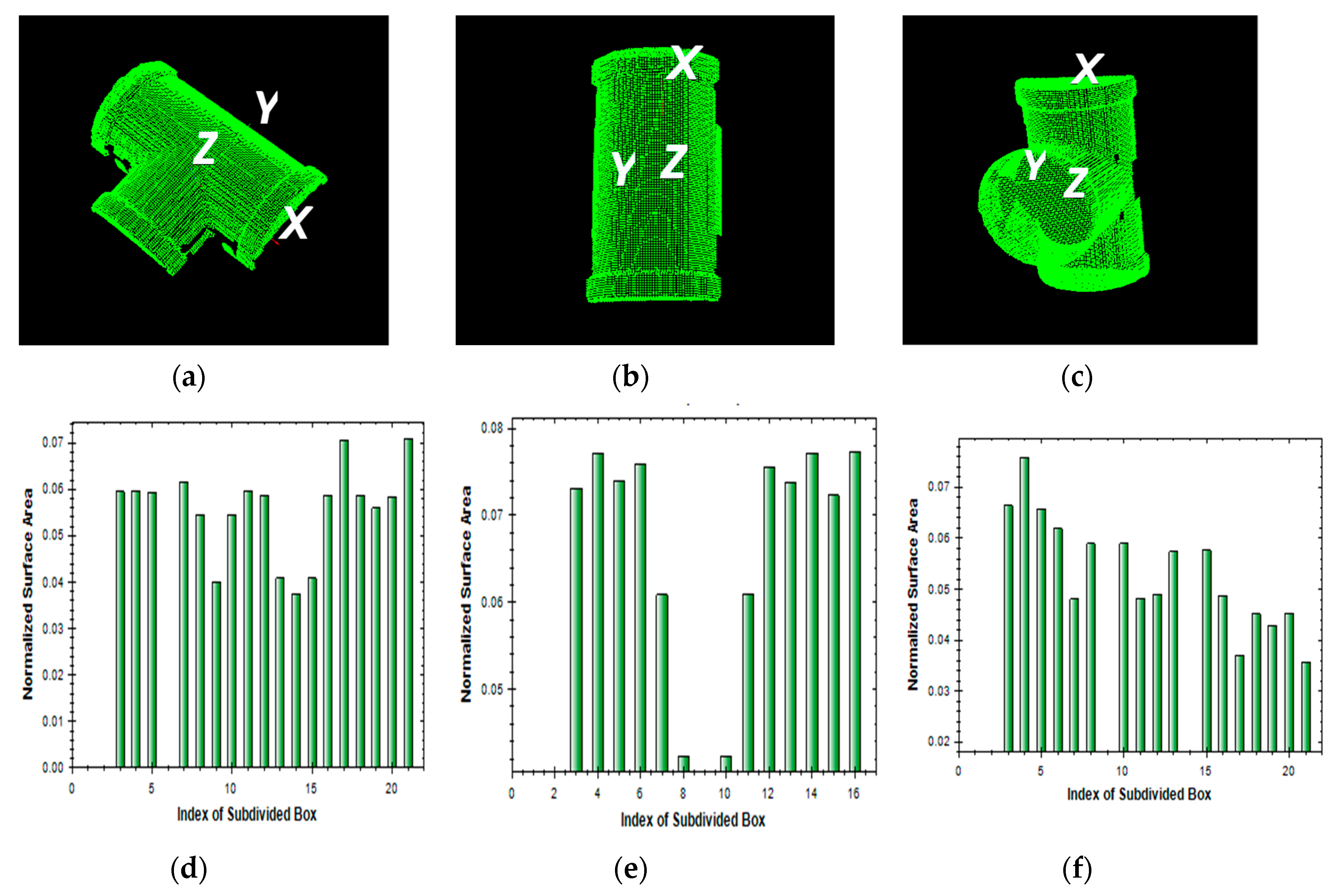
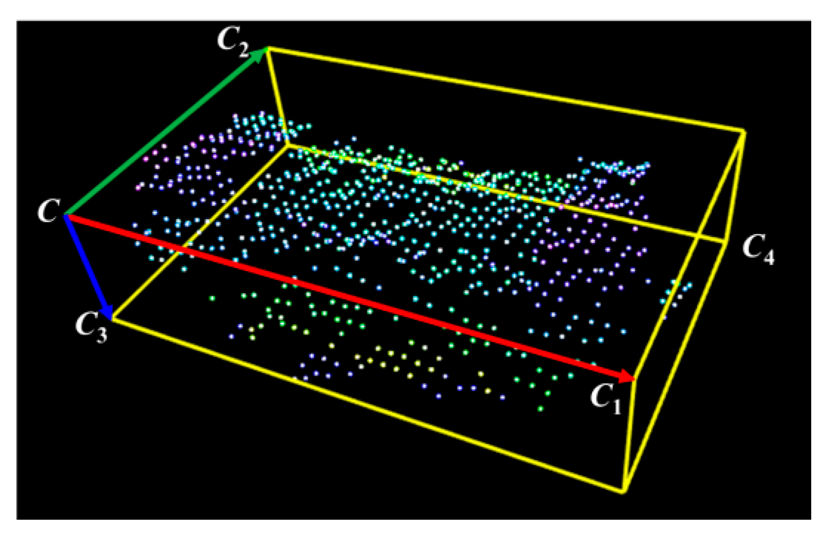
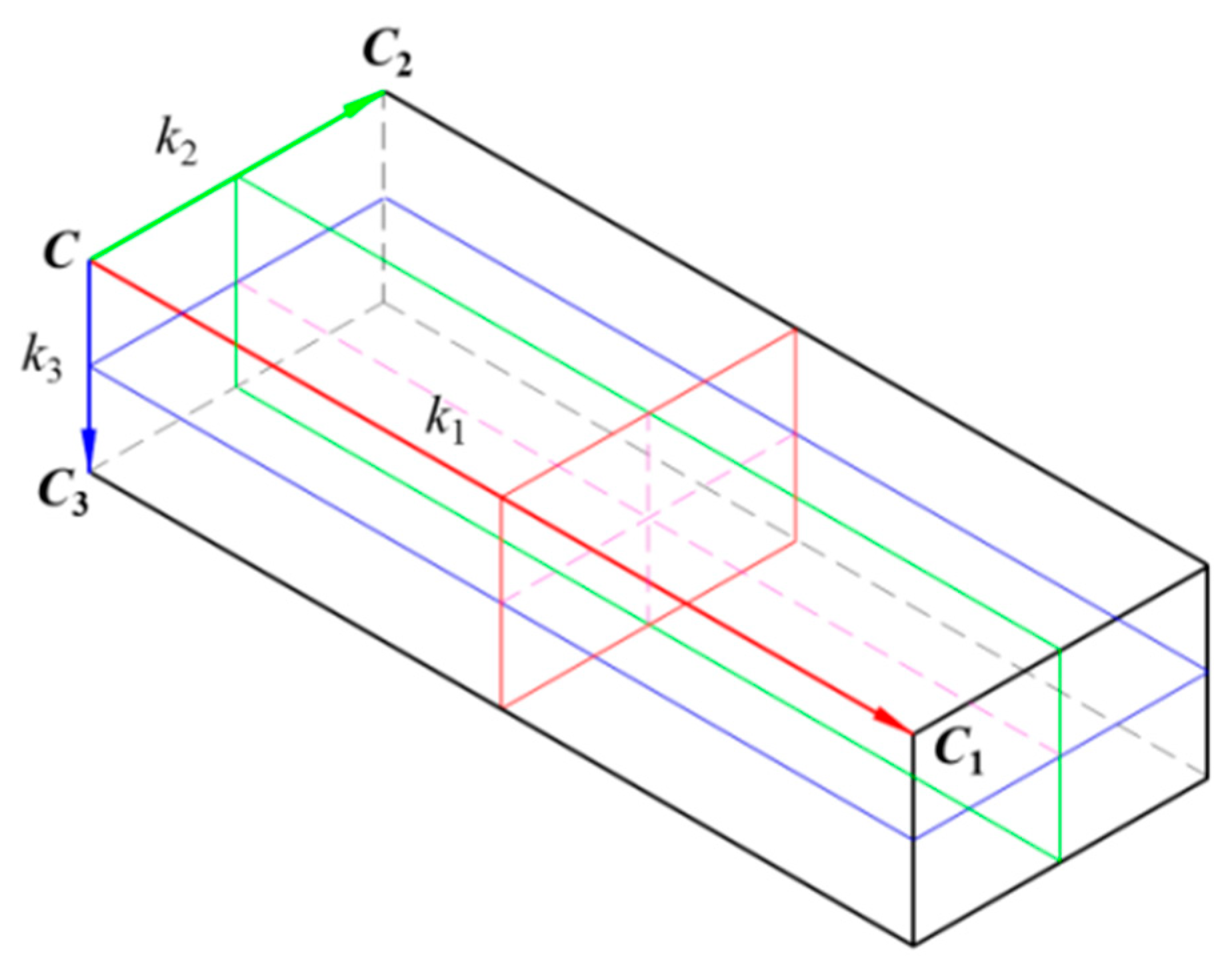
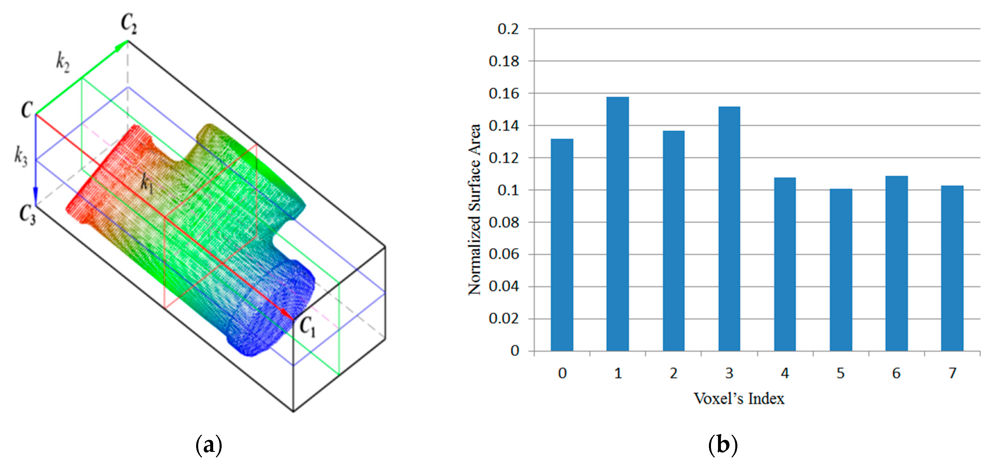
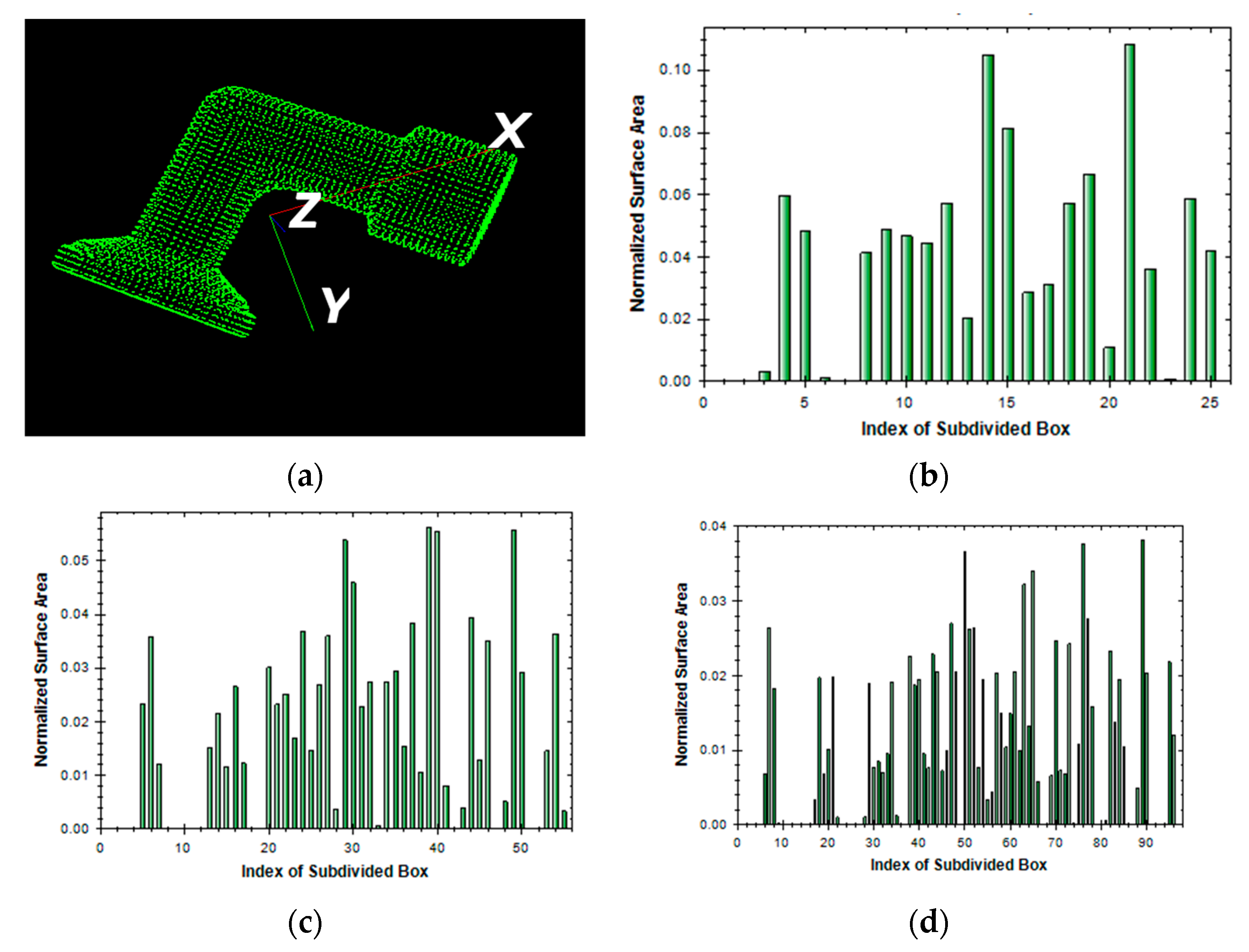
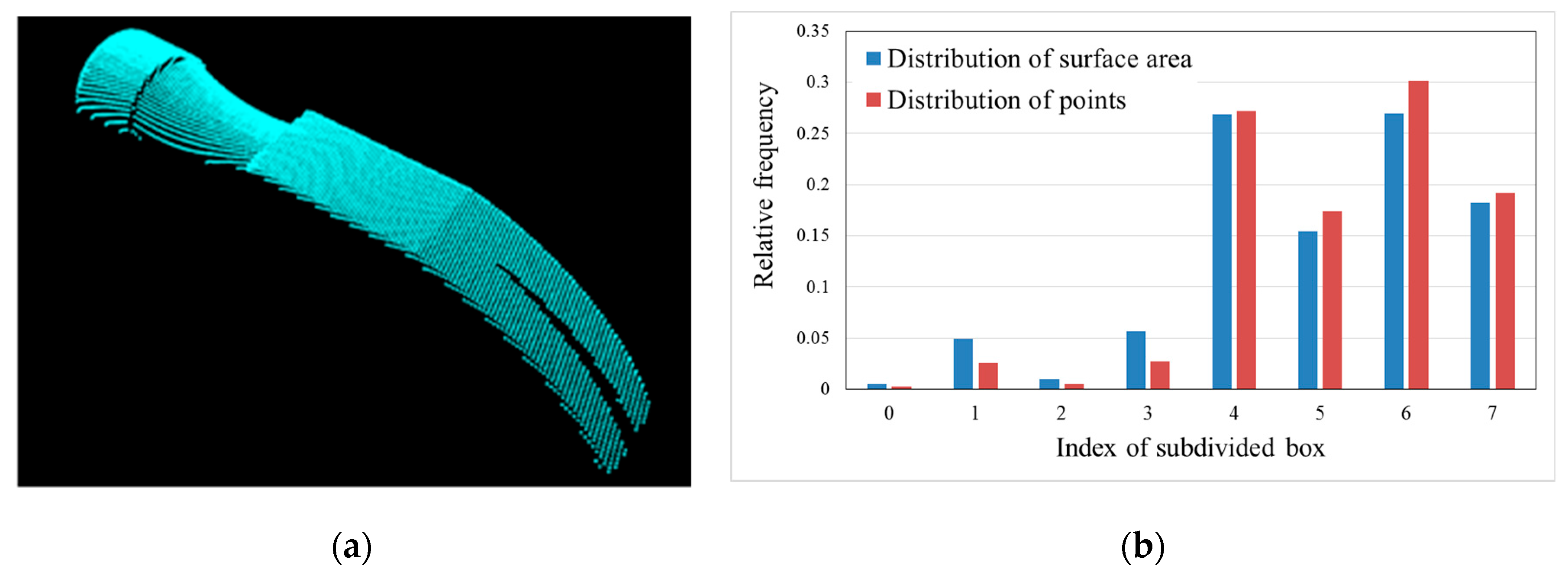
2.2. Regional Area-based Descriptor
- nV = k1k2k3 − 1;
- C: corner vector;
- CC1, CC2, and CC3: principle vectors corresponding to the maximum, middle, and minimum dimensions of the OBB, respectively.
2.2.1. Estimation of Oriented Bounding Box
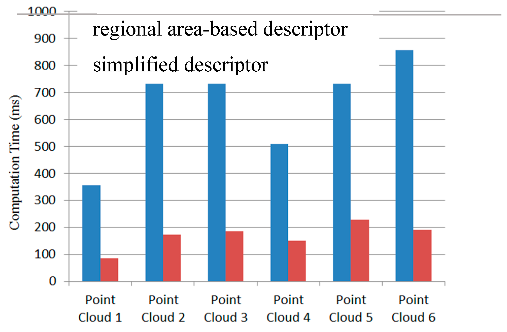
2.2.2. Simplified Regional Area-based Descriptor
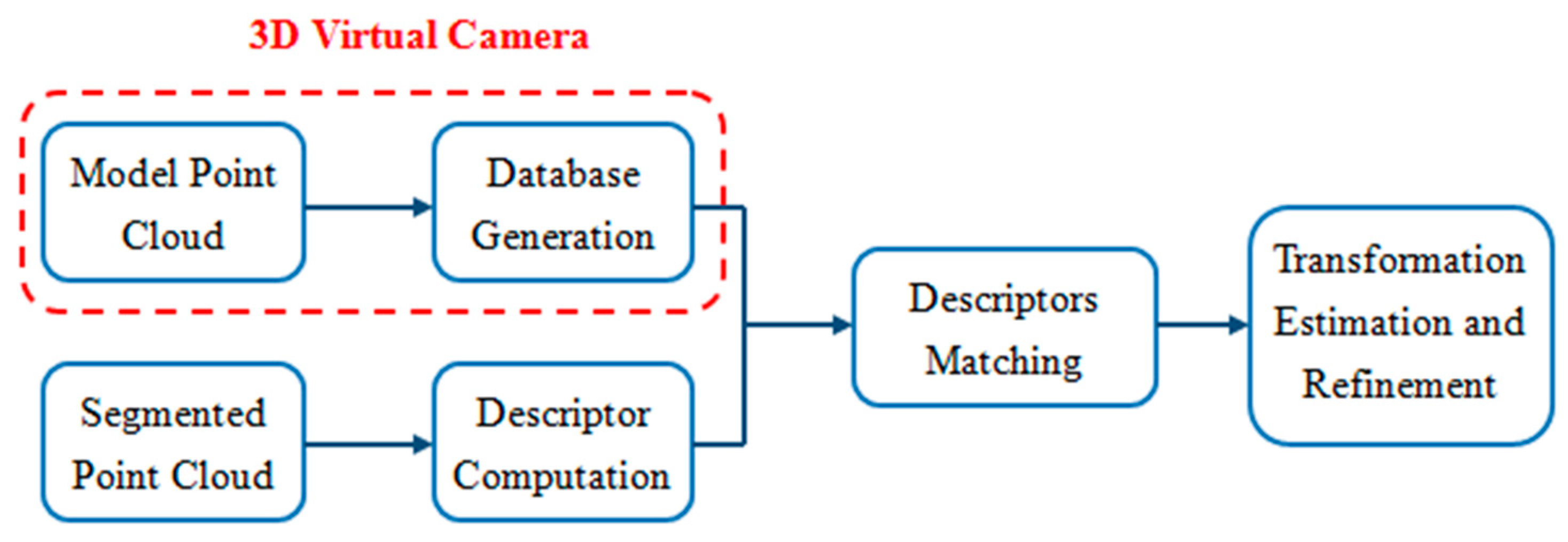
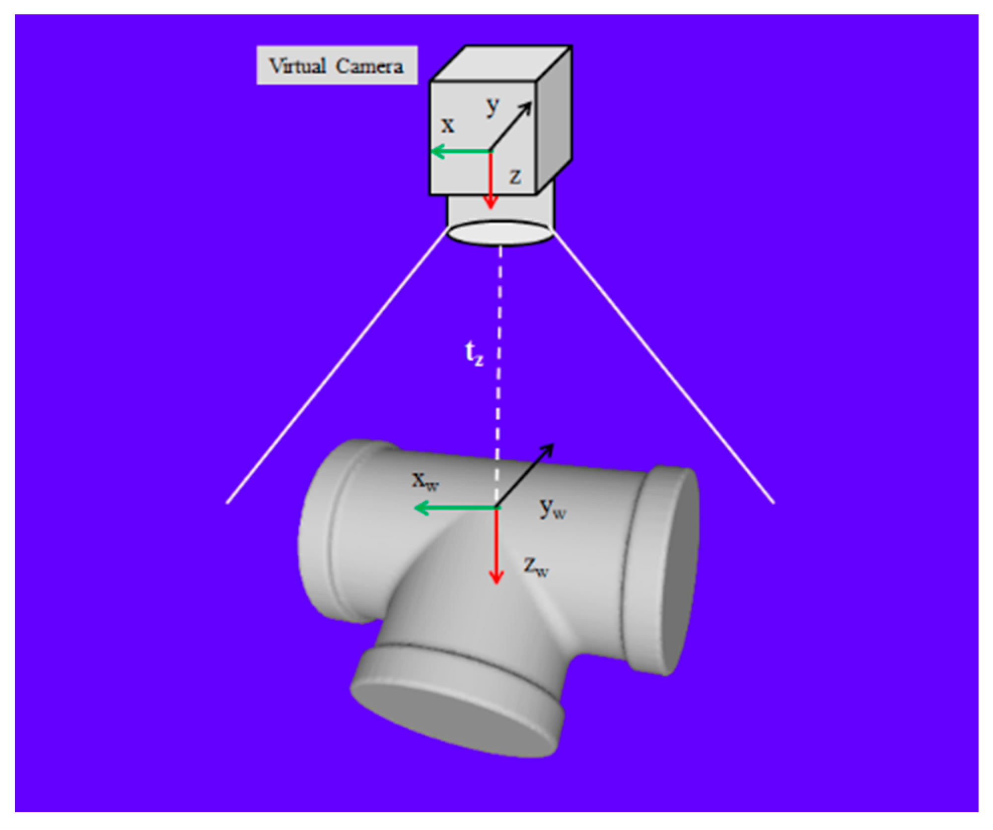
2.3. D Virtual Camera
2.4. Feature Matching
2.4.1. OBB Matching
2.4.2. Matching Criteria for Regional Area-based Descriptor
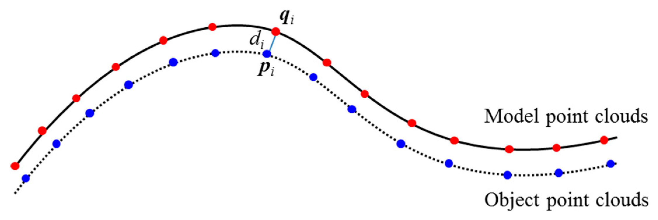
2.4.3. Transformation Estimation and Refinement
- For each point p ∈ O, find the closest point q ∈ M;
- Estimate the rotation matrix R and translation vector t that minimize the root mean squared distance;
- Transform Ok+1 ← Q(Ok) using the estimated parameters;
- Terminate the iteration when the change in error falls below the preset threshold.
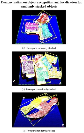
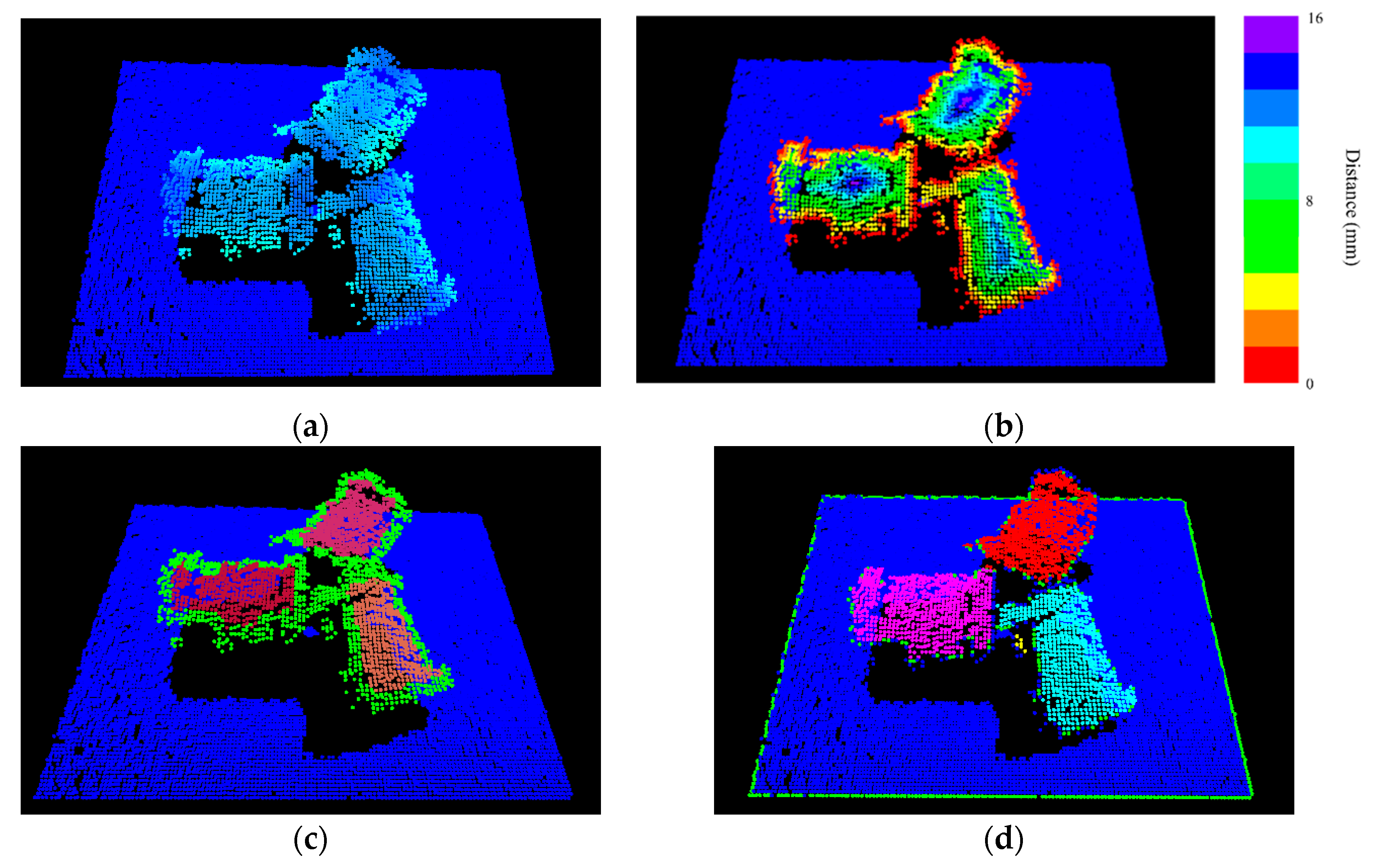
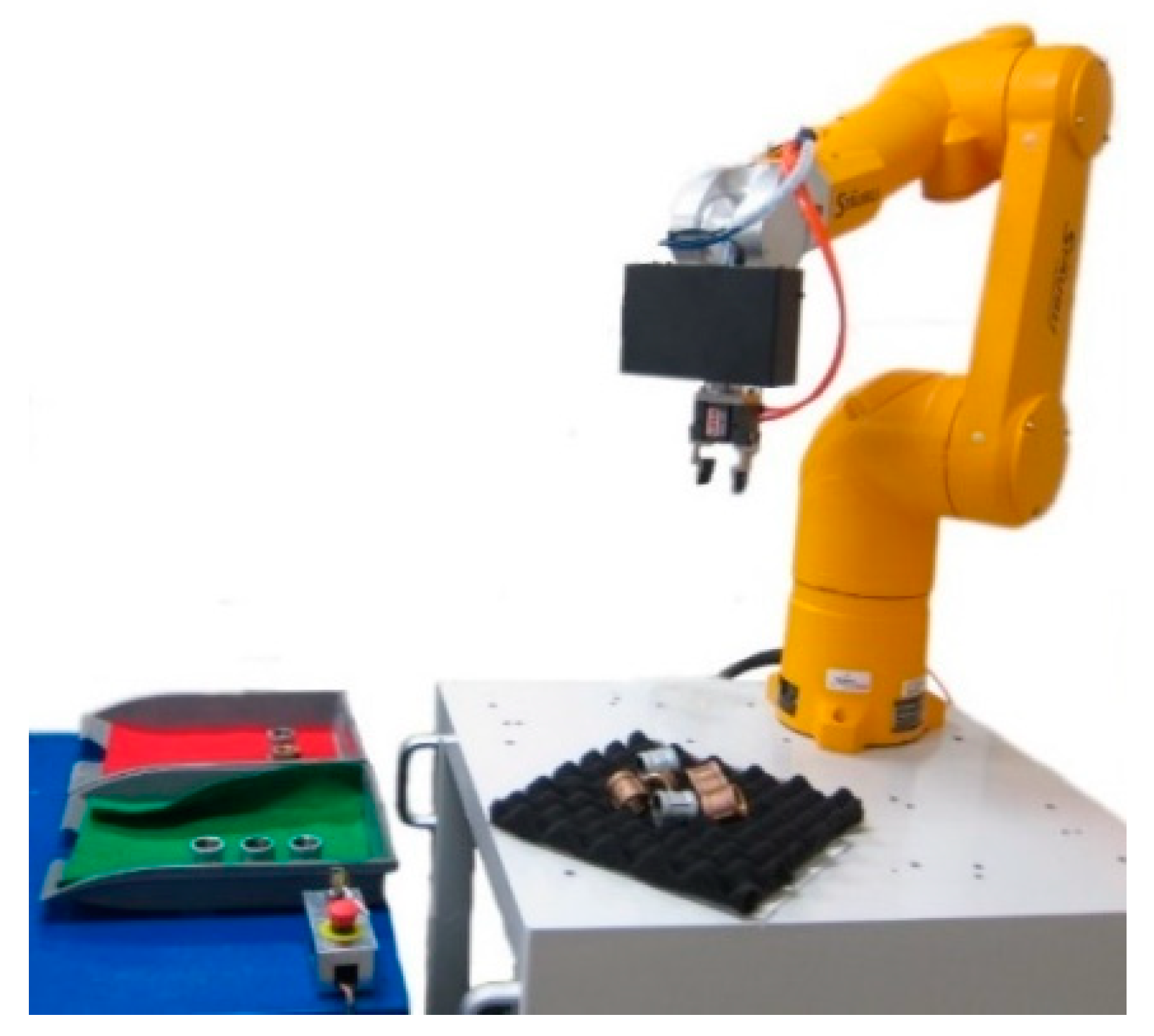
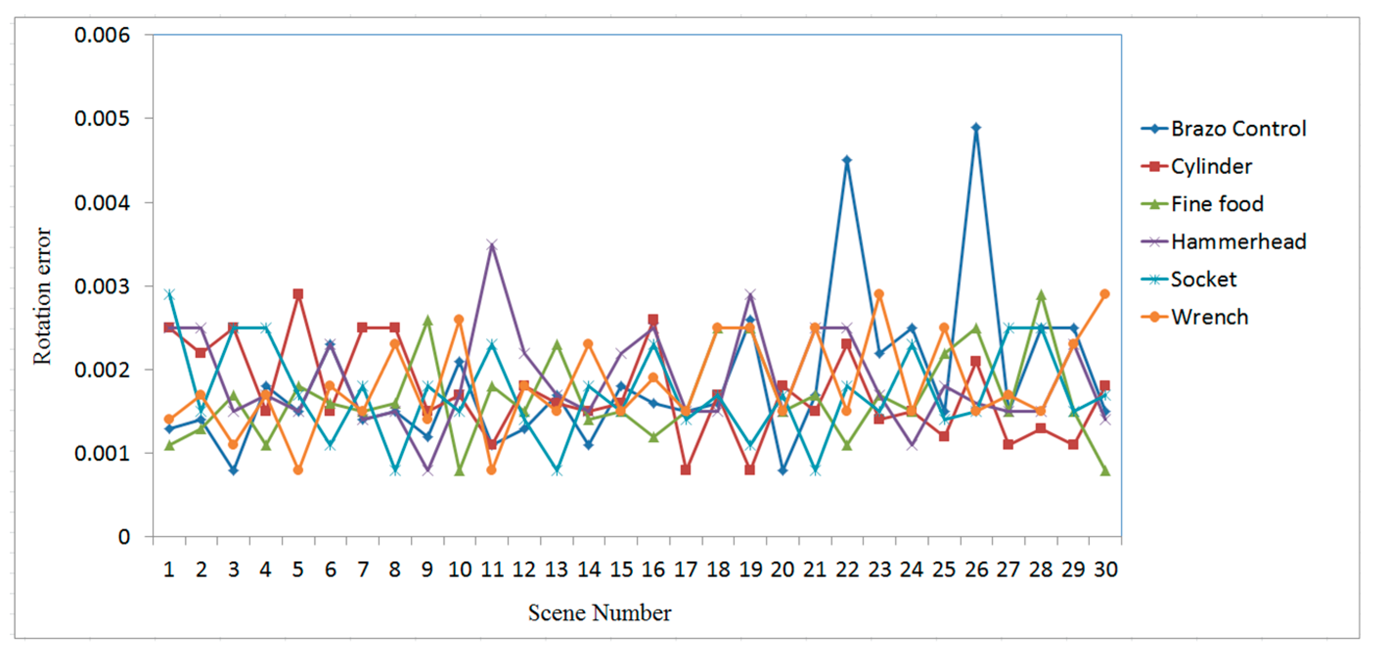
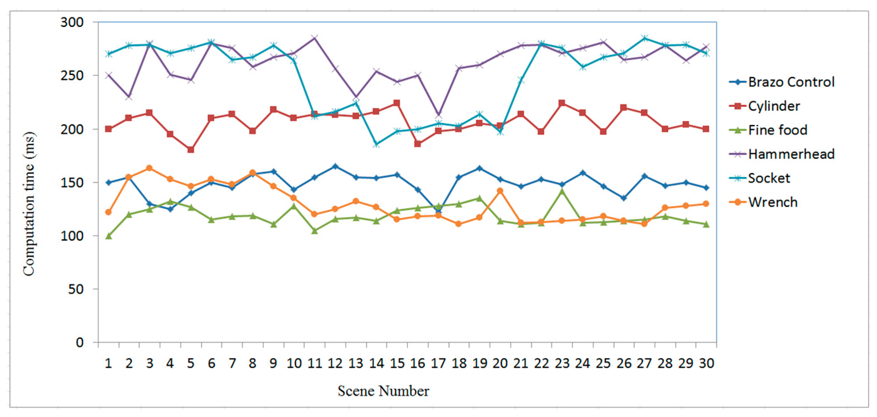
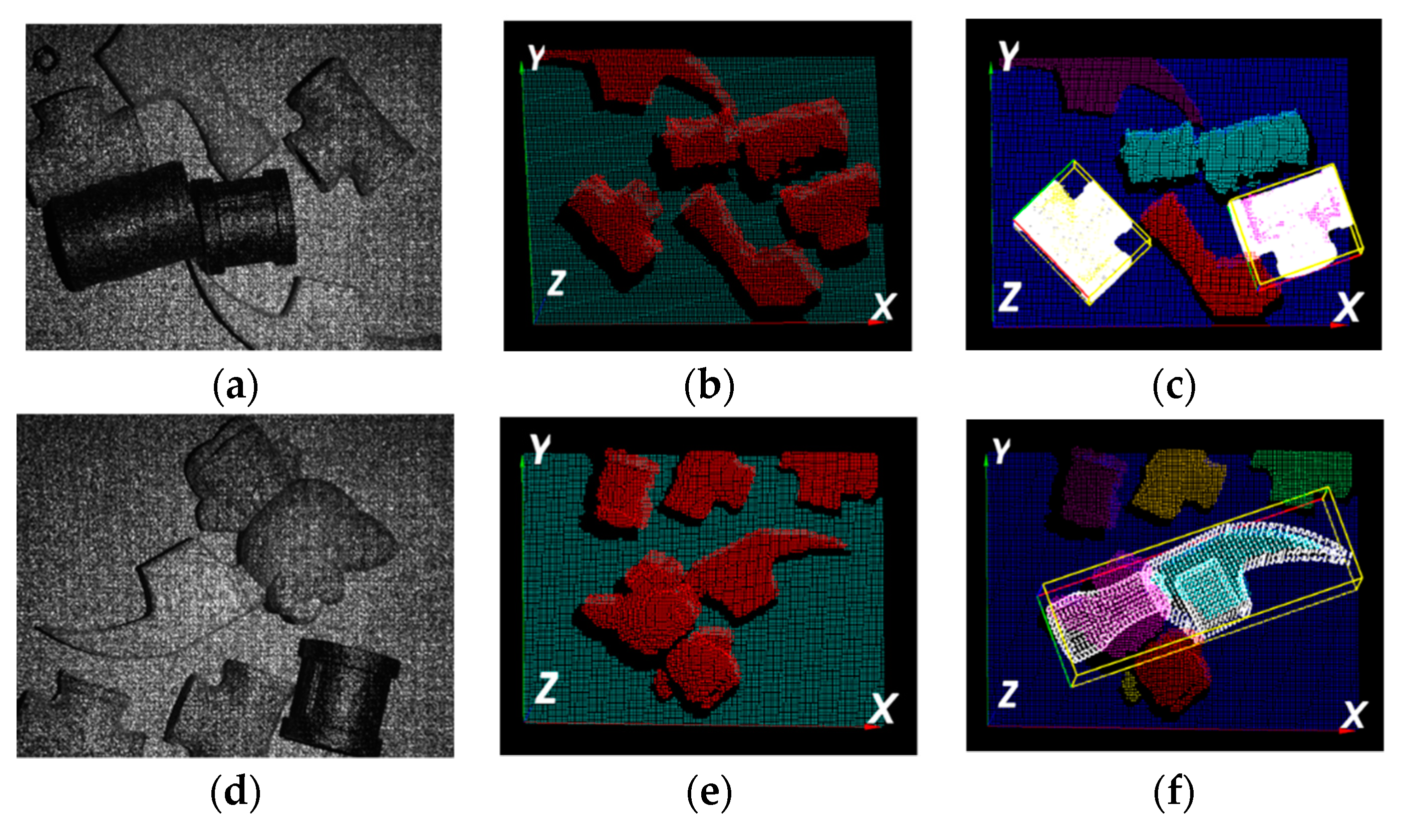
3. Experimental Results and Analysis
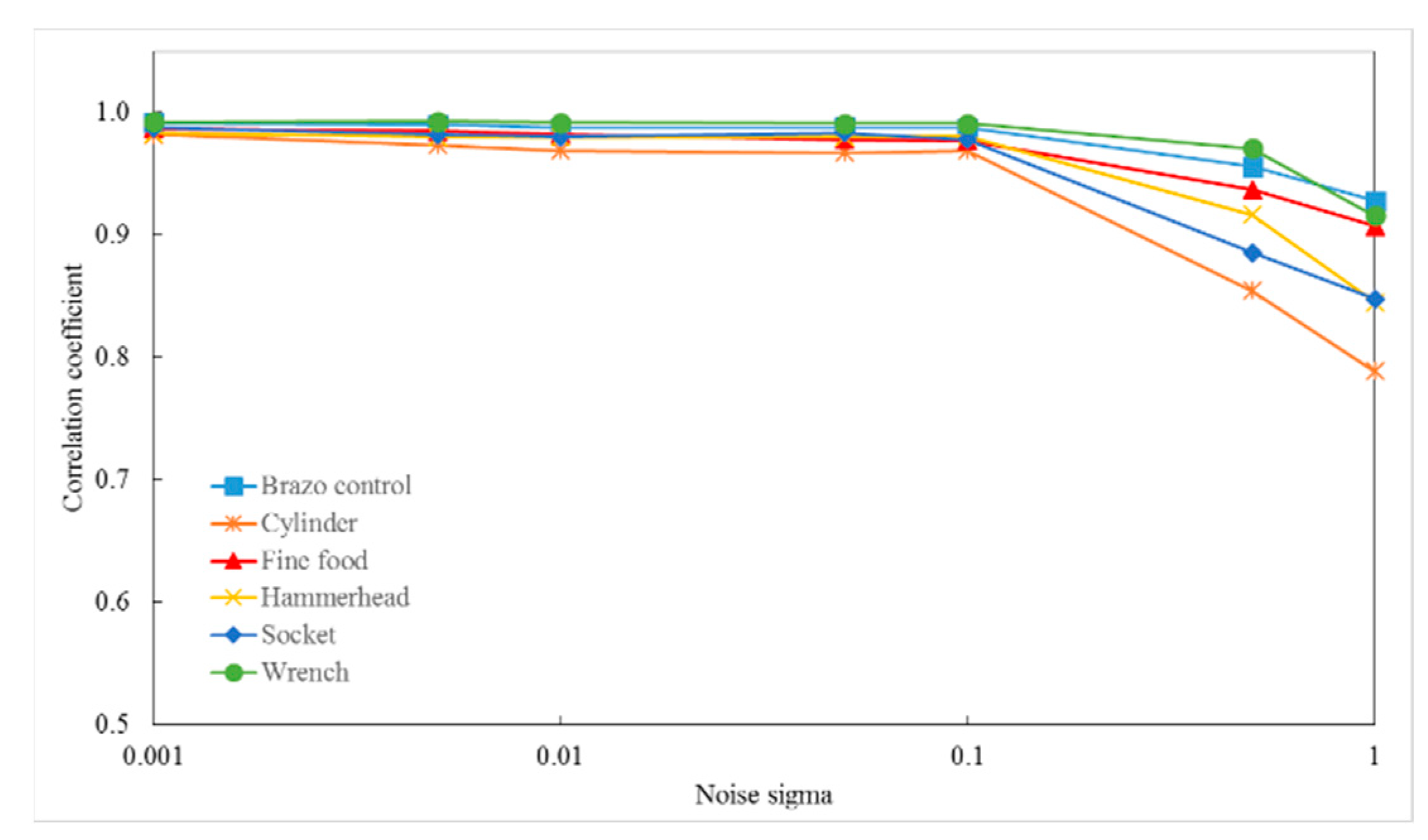
3.1. Case Study on Simulated Data
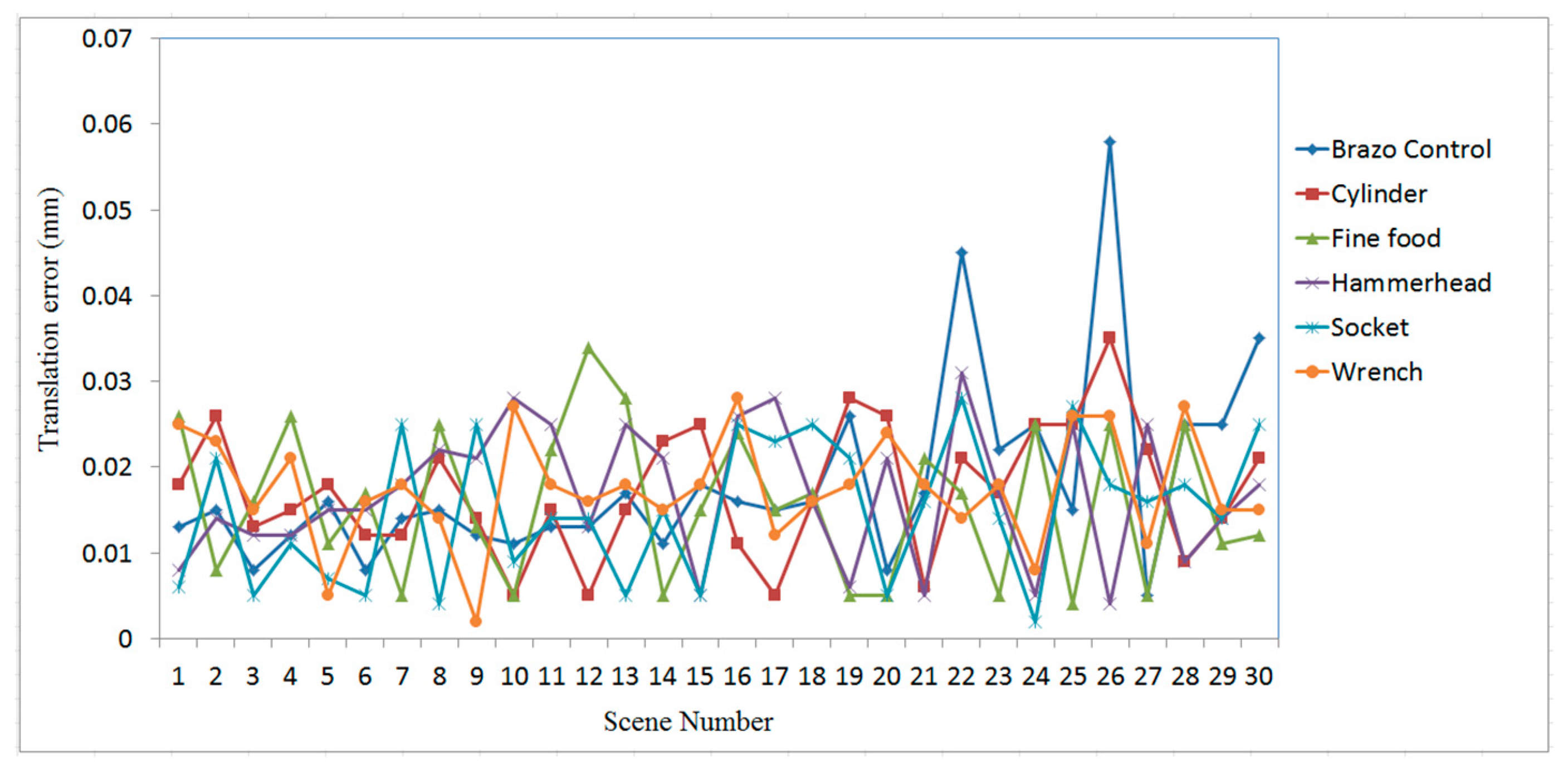
3.2. Case Study on Measured Data
4. Discussion
5. Conclusions
Author Contributions
Funding
Conflicts of Interest
References
- Birk, J.R.; Kelley, R.B.; Martins, H.A.S. An orienting robot for feeding workpieces stored in bins. IEEE Trans. Syst. Man Cybern. 1981, 11, 151–160. [Google Scholar] [CrossRef]
- Kelley, R.B.; Birk, J.R.; Martins, H.A.S.; Tella, R. A robot system which acquires cylindrical workpieces from bins. IEEE Trans. Syst. Man Cybern. 1982, 12, 204–213. [Google Scholar] [CrossRef]
- Torgerson, E.; Paul, F.W. Vision-guided robotic fabric manipulation for apparel manufacturing. IEEE Control Syst. Mag. 1988, 8, 14–20. [Google Scholar] [CrossRef]
- Cai, C.; Regtien, P.P.L. A smart sonar object recognition system for robots. Meas. Sci. Technol. 1993, 4, 95–100. [Google Scholar] [CrossRef]
- Kuehnle, J.; Verl, A.; Xue, Z.; Ruehl, S.; Zoellner, J.M.; Dillmann, R.; Grundmann, T.; Eidenberg, R.; Zoellner, R.D. 6D Object Localization and Obstacle Detection for Collision-Free Manipulation with a Mobile Service Robot. In Proceedings of the International Conference on Advanced Robotics, Munich, Germany, 22–26 June 2009; pp. 1–6. [Google Scholar]
- Fuchs, S.; Haddadin, S.; Keller, M.; Parusel, S.; Kolb, A.; Suppa, M. Cooperative Bin-Picking with Time-of-Flight Camera and Impedance Controlled DLR Lightweight Robot III. In Proceedings of the IEEE/RSJ International Conference on Intelligent Robots and Systems, Taipei, Taiwan, 18–22 October 2010; pp. 4862–4867. [Google Scholar]
- Skotheim, O.; Thielemann, J.T.; Berge, A.; Sommerfelt, A. Robust 3D Object Localization and Pose Estimation for Random Bin Picking with the 3DMaMa Algorithm. In Proceedings of the SPIE 7526 Three-Dimensional Image Processing and Application, San Jose, CA, USA, 4 February 2010; Volume 7526, p. 75260E. [Google Scholar]
- Liu, M.-Y.; Tuzel, O.; Veeraraghavan, A.; Taguchi, Y.; Marks, T.K.; Chellappa, R. Fast object localization and pose estimation in heavy clutter for robotic bin picking. Int. J. Rob. Res. 2012, 32, 951–973. [Google Scholar] [CrossRef]
- Skotheim, O.; Lind, M.; Ystgaard, P.; Fjerdingen, S.A. A Flexible 3D Object Localization System for Industrial Part Handling. Int. Robot. Syst. (IROS). In Proceedings of the IEEE/RSJ International Conference, Vilamoura, Portugal, 7–12 October 2012; pp. 3326–3333. [Google Scholar]
- Nieuwenhuisen, M.; Droeschel, D.; Holz, D.; Stuckler, J.; Berner, A.; Li, J.; Klein, R. Mobile Bin Picking with an Anthropomorphic Service Robot. In Proceedings of the IEEE International Conference on Robotics and Automation, Karlsruhe, Germany, 6–10 May 2013; pp. 2327–2334. [Google Scholar]
- Sansoni, G.; Bellandi, P.; Leoni, F.; Docchio, F. Optoranger: A 3D pattern matching method for bin picking applications. Opt. Lasers Eng. 2014, 54, 22–231. [Google Scholar] [CrossRef]
- Schnabel, R.; Wessel, R.; Wahl, R.; Klein, R. Shape Recognition in 3D Point-Clouds. In Proceedings of the 16th International Conference in Central Europe on Computer Graphics Visualization and Computer Vision, Plzen, Czech Republic, 4–7 February 2008. [Google Scholar]
- Johnson, A.E.; Hebert, M. Surface matching for object recognition in complex three-dimensional scenes. Image Vis Comput. 1998, 16, 635–651. [Google Scholar] [CrossRef]
- Chen, H.; Bhanu, B. 3D free-form object recognition in range images using local surface patches. Pattern Recogn. Lett. 2007, 28, 1252–1262. [Google Scholar] [CrossRef]
- Zaharescu, A.; Boyer, E.; Varanasi, K.; Horaud, R. Surface Feature Detection and Description with Applications to Mesh Matching. In Proceedings of the IEEE Conference on Computer Vision adn Pattern Recognition, Miami, FL, USA, 20–25 June 2009; pp. 373–380. [Google Scholar]
- Drost, B.; Ulrich, M.; Navab, N.; Ilic, S. Model Globally, Match Locally: Efficient and Robust 3D Object Recognition. In Proceedings of the IEEE Conference on Computer Vision and Pattern Recognition, San Francisco, CA, USA, 13–18 June 2010; pp. 998–1005. [Google Scholar]
- Rusu, R.B.; Bradski, G.; Thibaux, R.; Hsu, J. Fast 3D recognition and pose using the Viewpoint Feature Histogram. In Proceedings of the IEEE/RSJ International Conference on Intelligent Robots and System, Taipei, Taiwan, 18–22 October 2010; pp. 2155–2162. [Google Scholar]
- Salti, S.; Tombari, F.; Di Stefano, L. SHOT: Unique signatures of histograms for surface and texture description. Comput. Vis Image Underst. 2014, 125, 251–264. [Google Scholar] [CrossRef]
- Le, V.-H.; Le, T.-L.; Vu, H.; Nguyen, T.T.; Tran, T.-H.; Dao, T.-C.; Nguyen, H.-Q. Geometry-Based 3D Object Fitting and Localizing in Grasping Aid for Visually Impaired. In Proceedings of the IEEE Interntional Conference on Consumer Electronics (ICCE), Mumbai, India, 7–11 January 2016; p. 1. [Google Scholar]
- Dantanarayana, H.G.; Huntley, J.M. Object recognition and localization from 3D point clouds by maximum-likelihood estimation. R Soc. Open Sci. 2017, 4, 160693. [Google Scholar] [CrossRef] [PubMed]
- Chen, L.-C.; Hong, H.; Nguyen, X.-L.; Wu, H.-W. Novel 3-D object recognition methodology employing a curvature-based histogram. Int. J. Adv. Robot Syst. 2013. [Google Scholar] [CrossRef]
- Chen, L.-C.; Nguyen, T.-H.; Lin, S.-T. Viewpoint-independent. 3D object segmentation for randomly stacked objects using optical object detection. Meas. Sci. Technol. 2015, 26, 105202. [Google Scholar]
- Rabbani, T.; van den Heuvel, F.A.; Vosselman, G. Segmentation of point clouds using smoothness constraint. Int. Arch. Photogramm. Remote Sens. Spat. Inf. Sci. 2006, 35, 248–253. [Google Scholar]
- Nurunnabi, A.; Belton, D.; West, G. Robust Segmentation in Laser Scanning 3D Point Cloud Data. In Proceedings of the International Conference on Digital Image Computing Techniques and Applications, Fremantle, WA, Australia, 2–5 December 2012; pp. 1–8. [Google Scholar]
- Rusu, R.B.; Blodow, N.; Marton, Z.C.; Beetz, M. Close-Range Scene Segmentation and Reconstruction of 3D Point Cloud Maps for Mobile Manipulation in Domestic Environments. In Proceedings of the IEEE/RSJ International Conference on Intelligent Robots and Systems, St. Louis, MO, USA, 10–15 October 2009; pp. 1–6. [Google Scholar]
- Douillard, B.; Underwood, J.; Kuntz, N.; Vlaskine, V.; Quadros, A.; Morton, P.; Frenkel, A. On the Segmentation of 3D LIDAR Point Clouds. In Proceedings of the IEEE International Conference on. Robotics and Automation, Shanghai, China, 9–13 May 2011; pp. 2798–2805. [Google Scholar]
- Anguelov, D.; Taskarf, B.; Chatalbashev, V.; Koller, D.; Gupta, D.; Heitz, G.; Ng, A. Discriminative Learning of Markov Random Fields for Segmentation of 3D Scan Data. In Proceedings of the IEEE Computer Society Conference on Computer Vision and Pattern Recognition, San Diego, CA, USA, 20–25 June 2005; Volume 2, pp. 169–176. [Google Scholar]
- Golovinskiy, A.; Funkhouser, T. Min-Cut Based Segmentation of Point Clouds. In Proceedings of the IEEE International Conference on Computer Vision and Workshop, Kyoto Japan, 27 September–4 October 2009; pp. 39–46. [Google Scholar]
- Munoz, D.; Vandapel, N.; Hebert, M. Onboard Contextual Classification of 3-D Point Clouds with Learned High-Order Markov Random Fields. In Proceedings of the IEEE International Conference on Robotics an Automation, Kobe, Japan, 12–17 May 2009; pp. 2009–2016. [Google Scholar]
- Chen, L.-C.; Hoang, D.-C.; Lin, H.-I.; Nguyen, T.-H. Innovative methodology for multi-view point clouds registration in robotic 3-D object scanning and reconstruction. Appl. Sci. 2016, 6, 132. [Google Scholar] [CrossRef]
- Gottschalk, S.; Lin, M.C.; Manocha, D. OBBTree: A Hierarchical Structure for Rapid Interference Detection. In Proceedings of the 23rd Annual Conference on Computer Graphics and Interactive Technique, New Orleans, LA, USA, 4–9 August 1996; pp. 171–180. [Google Scholar]
- Besl, P.J.; McKay, N.D. A method for registration of 3-D shapes. IEEE Trans. Pattern. Anal. Mach. Intell. 1992, 14, 239–256. [Google Scholar] [CrossRef]
- Marton, Z.C.; Rusu, R.B.; Beetz, M. On Fast Surface Reconstruction Methods for Large and Noisy Point clouds. In Proceedings of the IEEE International Conference on Robotics and Automation, Kobe, Japan, 12–17 May 2009; pp. 3218–3223. [Google Scholar]
- Krebs, B.; Sieverding, P.; Korn, B. A Fuzzy ICP Algorithm for 3D Free-Form Object Recognition. In Proceedings of the 13th International Conference on Pattern Recognition, Vienna, Austria, 25–29 August 1996; Volume 1, pp. 539–543. [Google Scholar]


| Model | Dimensions (mm) | |||
|---|---|---|---|---|
| Name | 3-D representation | Length | Width | Height |
| Brazo control |  | 86 | 53 | 30 |
| Cylinder |  | 35 | 35 | 35 |
| Finefood |  | 41 | 40 | 33 |
| Hammerhead |  | 110 | 35.5 | 22 |
| Socket |  | 45 | 35 | 35 |
| Wrench |  | 154 | 65 | 13.2 |
| Models | Method | Translation Error (mm) | Rotation Error (10−3 rad) | Time (s) |
|---|---|---|---|---|
| Fine food | Graph-based | 0.869 | 0.103 | 2.537 |
| Feature-based | 0.412 | 0.072 | 1.453 | |
| View-based | 0.036 | 0.087 | 7.521 | |
| Proposed | 0.019 | 0.068 | 0.160 | |
| Cylinder | Graph-based | 0.435 | 0.145 | 4.896 |
| Feature-based | 0.132 | 0.768 | 2.902 | |
| View-based | 0.038 | 0.108 | 8.247 | |
| Proposed | 0.022 | 0.061 | 0.182 | |
| Wrench | Graph-based | 0.213 | 0.315 | 4.184 |
| Feature-based | 0.896 | 0.979 | 3.262 | |
| View-based | 0.078 | 0.113 | 9.163 | |
| Proposed | 0.017 | 0.081 | 0.150 |
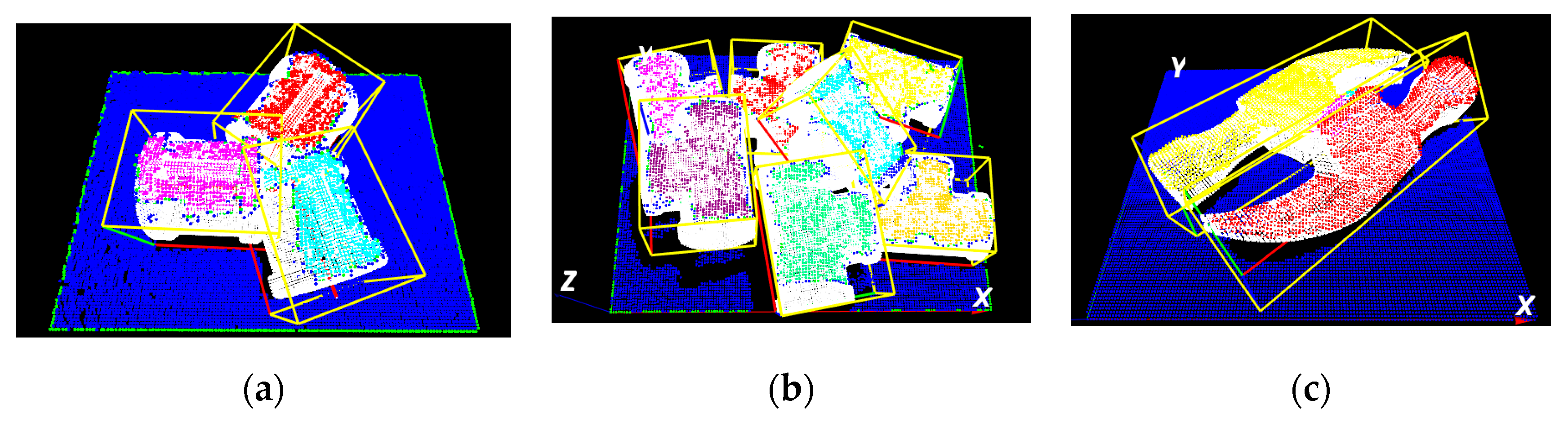
| Case study | Object | Matching Score (%) | Mean Deviation µ (mm) | Standard Deviation σ (mm) |
|---|---|---|---|---|
| 1 | Red | 89.74 | 0.320 | 0.392 |
| Magenta | 90.12 | 0.389 | 0.426 | |
| Cyan | 85.55 | 0.469 | 0.484 | |
| 2 | Red | 98.77 | 0.249 | 0.313 |
| Yellow | 99.23 | 0.187 | 0.242 | |
| Magenta | 97.55 | 0.247 | 0.316 | |
| Cyan | 92.88 | 0.351 | 0.431 | |
| Purple | 91.74 | 0.329 | 0.394 | |
| Gold | 98.55 | 0.231 | 0.305 | |
| Spring green | 94.57 | 0.313 | 0.372 | |
| 3 | Red | 98.31 | 0.266 | 0.264 |
| Yellow | 99.26 | 0.180 | 0.168 | |
| Average: | 94.69 | 0.294 | 0.342 | |
© 2019 by the authors. Licensee MDPI, Basel, Switzerland. This article is an open access article distributed under the terms and conditions of the Creative Commons Attribution (CC BY) license (http://creativecommons.org/licenses/by/4.0/).
Share and Cite
Chen, L.-C.; Nguyen, T.-H. A Novel Surface Descriptor for Automated 3-D Object Recognition and Localization. Sensors 2019, 19, 764. https://doi.org/10.3390/s19040764
Chen L-C, Nguyen T-H. A Novel Surface Descriptor for Automated 3-D Object Recognition and Localization. Sensors. 2019; 19(4):764. https://doi.org/10.3390/s19040764
Chicago/Turabian StyleChen, Liang-Chia, and Thanh-Hung Nguyen. 2019. "A Novel Surface Descriptor for Automated 3-D Object Recognition and Localization" Sensors 19, no. 4: 764. https://doi.org/10.3390/s19040764
APA StyleChen, L.-C., & Nguyen, T.-H. (2019). A Novel Surface Descriptor for Automated 3-D Object Recognition and Localization. Sensors, 19(4), 764. https://doi.org/10.3390/s19040764