Visual Calibration for Multiview Laser Doppler Speed Sensing

Abstract
1. Introduction
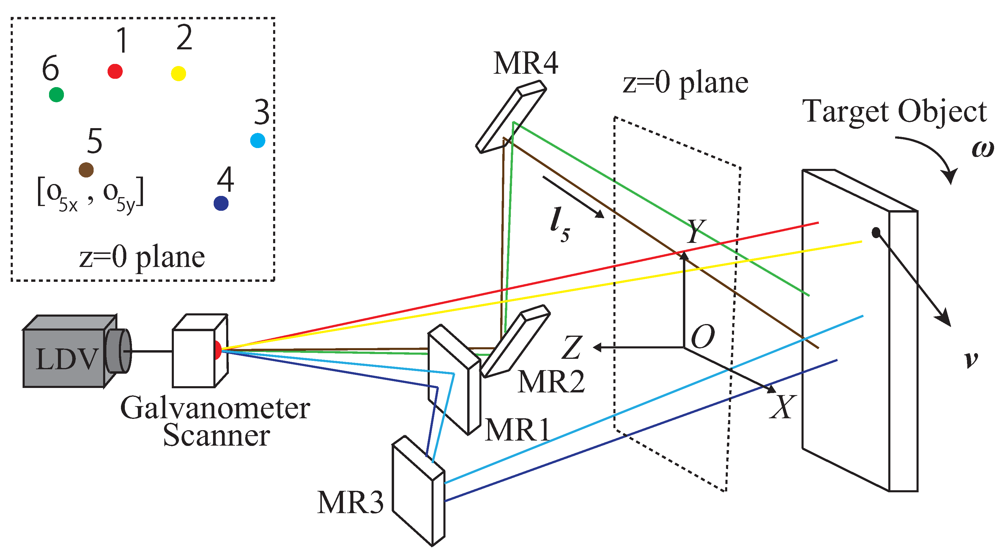
2. MLDSS Parameters
Basic Equations
3. MLDSS Calibration
3.1. Geometric-Only Calibration
3.2. Statistical Calibration by Minimizing Motion-Reconstruction Error
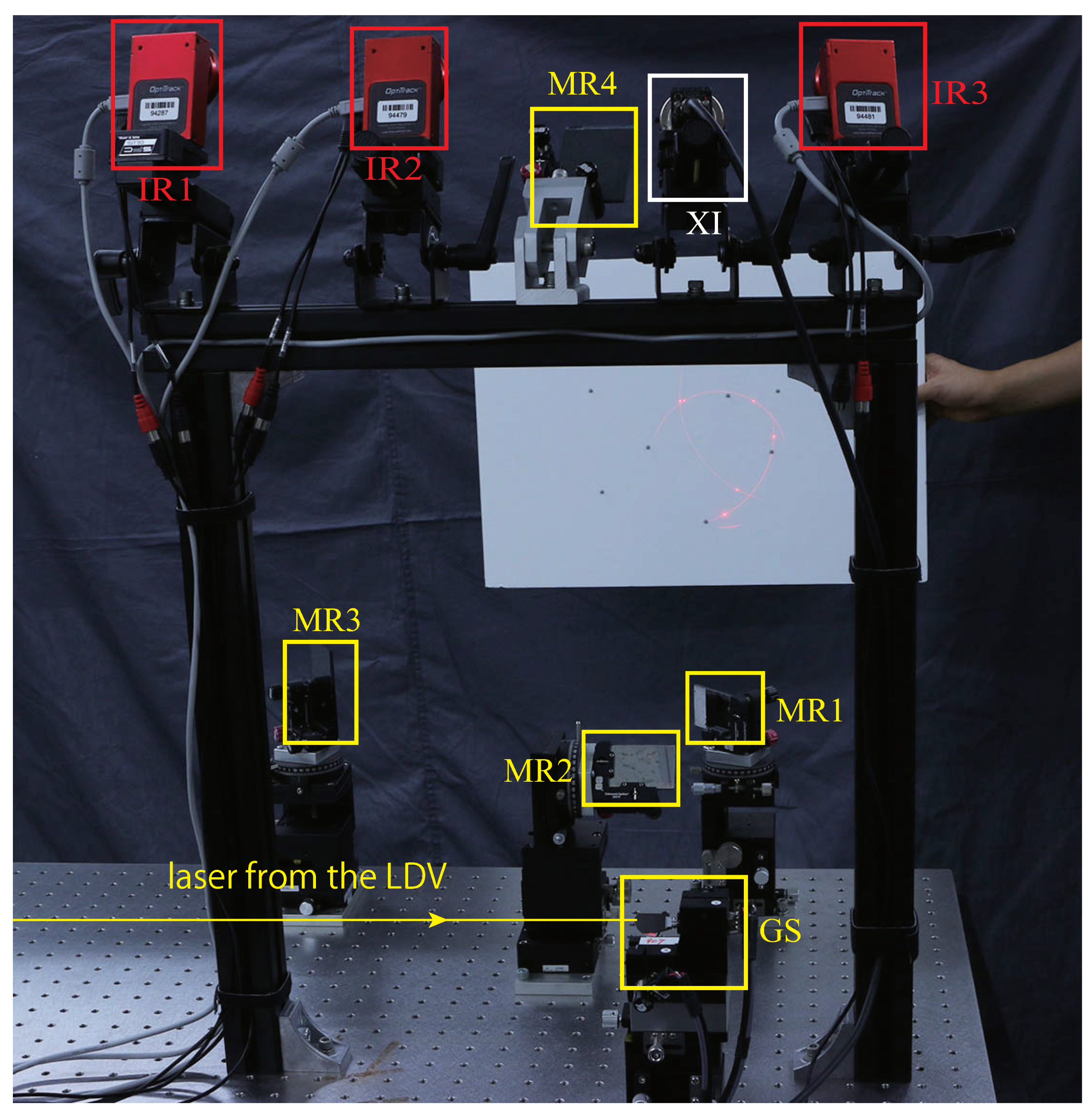
3.3. System Setup and Nonideal Factors
3.4. Summary
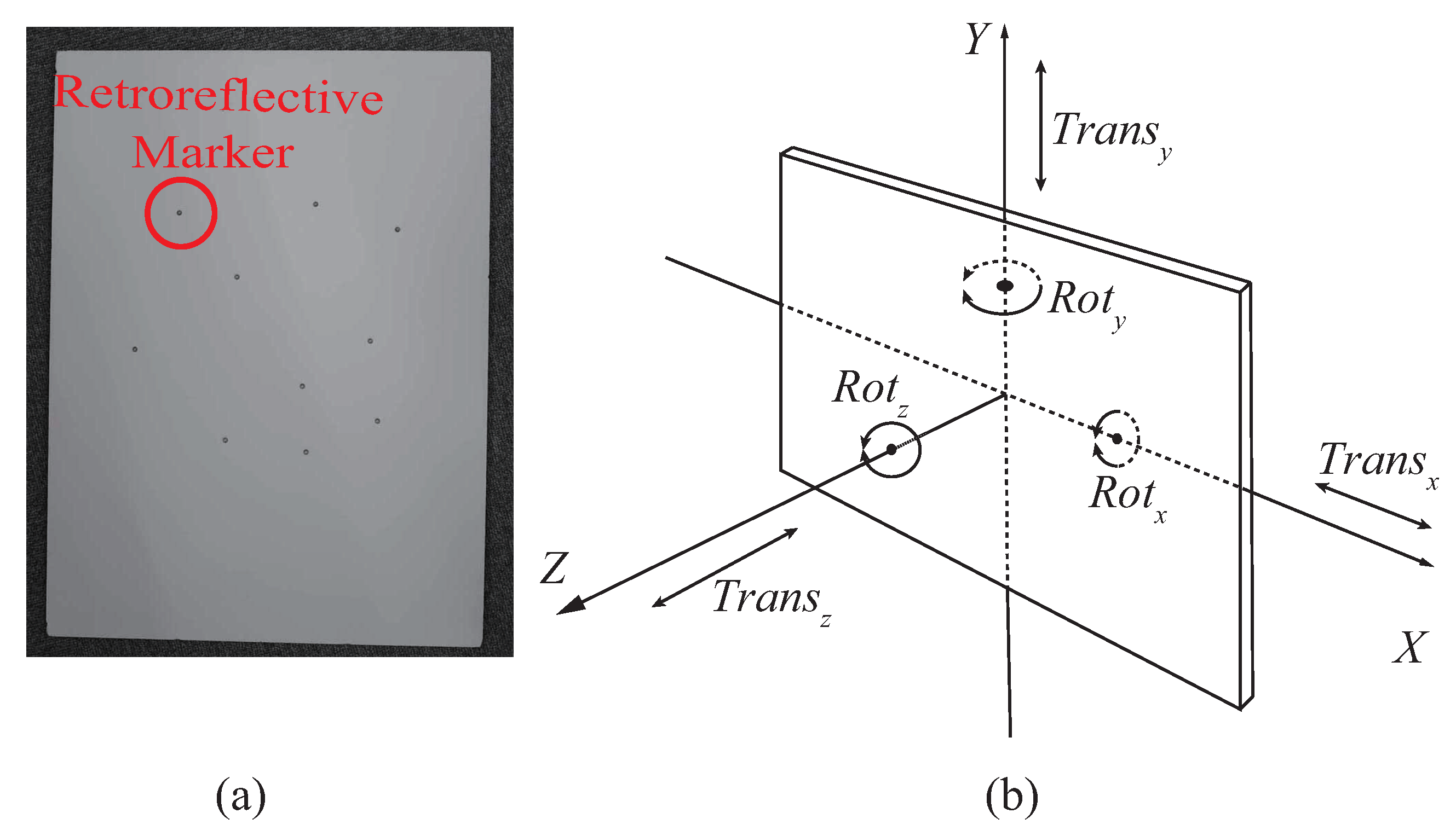
- Make a calibration object with four or more asymmetric placed markers;
- register the calibration object in the 3D tracking system as a trackable rigid body;
- simultaneously capture target motion and speed with the MLDSS and the 3D tracking system, and build a dataset following the instructions in Section 4;
- estimate initial parameters using the geometric-only method introduced in Section 3.1 (optional); and
- refine all parameters by solving Equation (13).
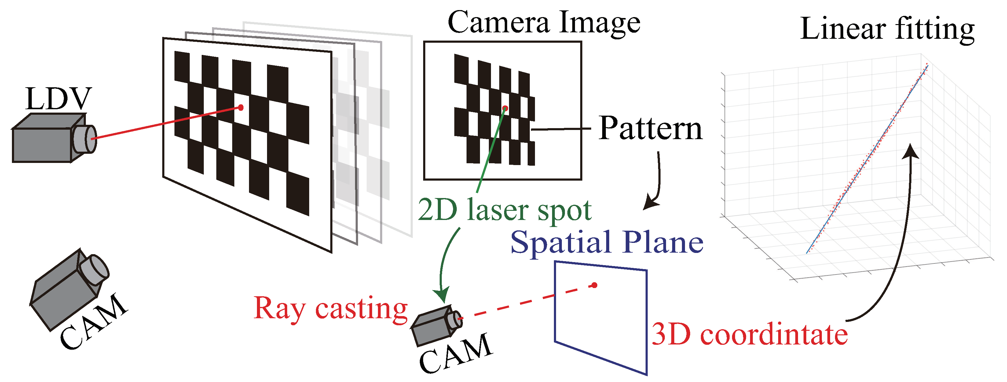
4. Data Collection
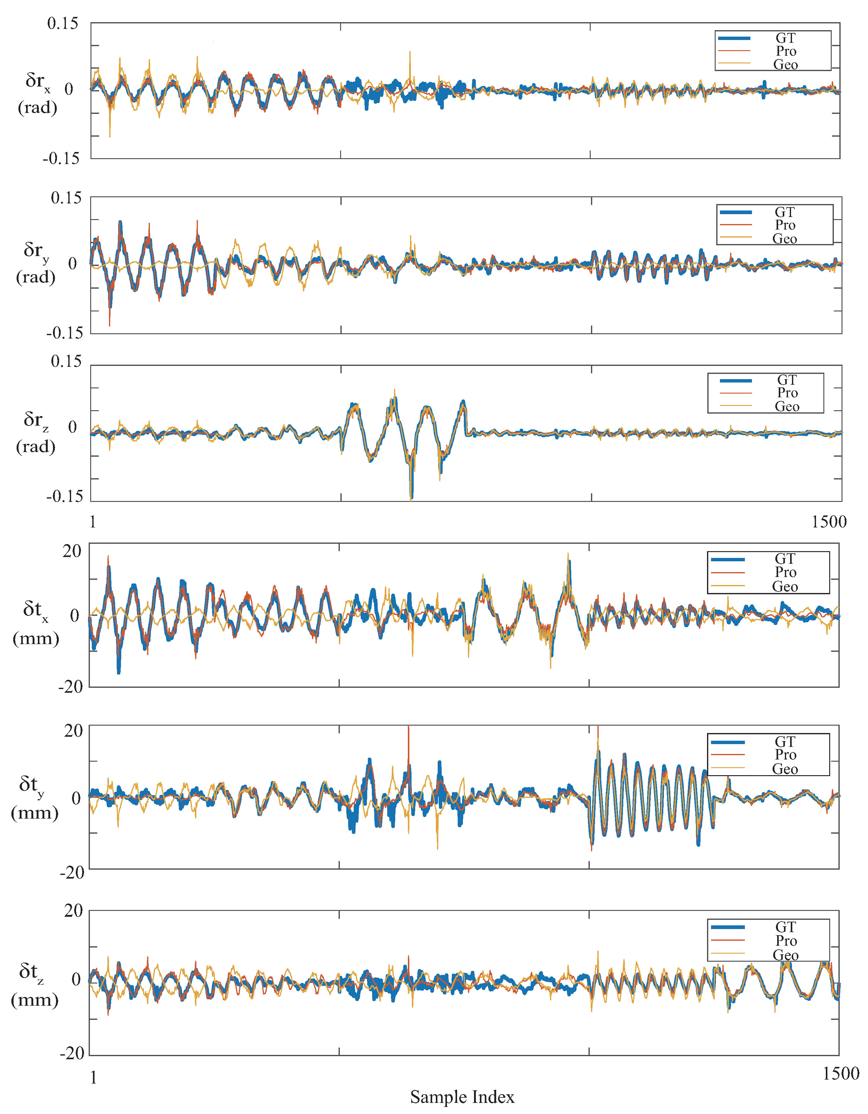
5. Evaluation
5.1. Cross-Validation
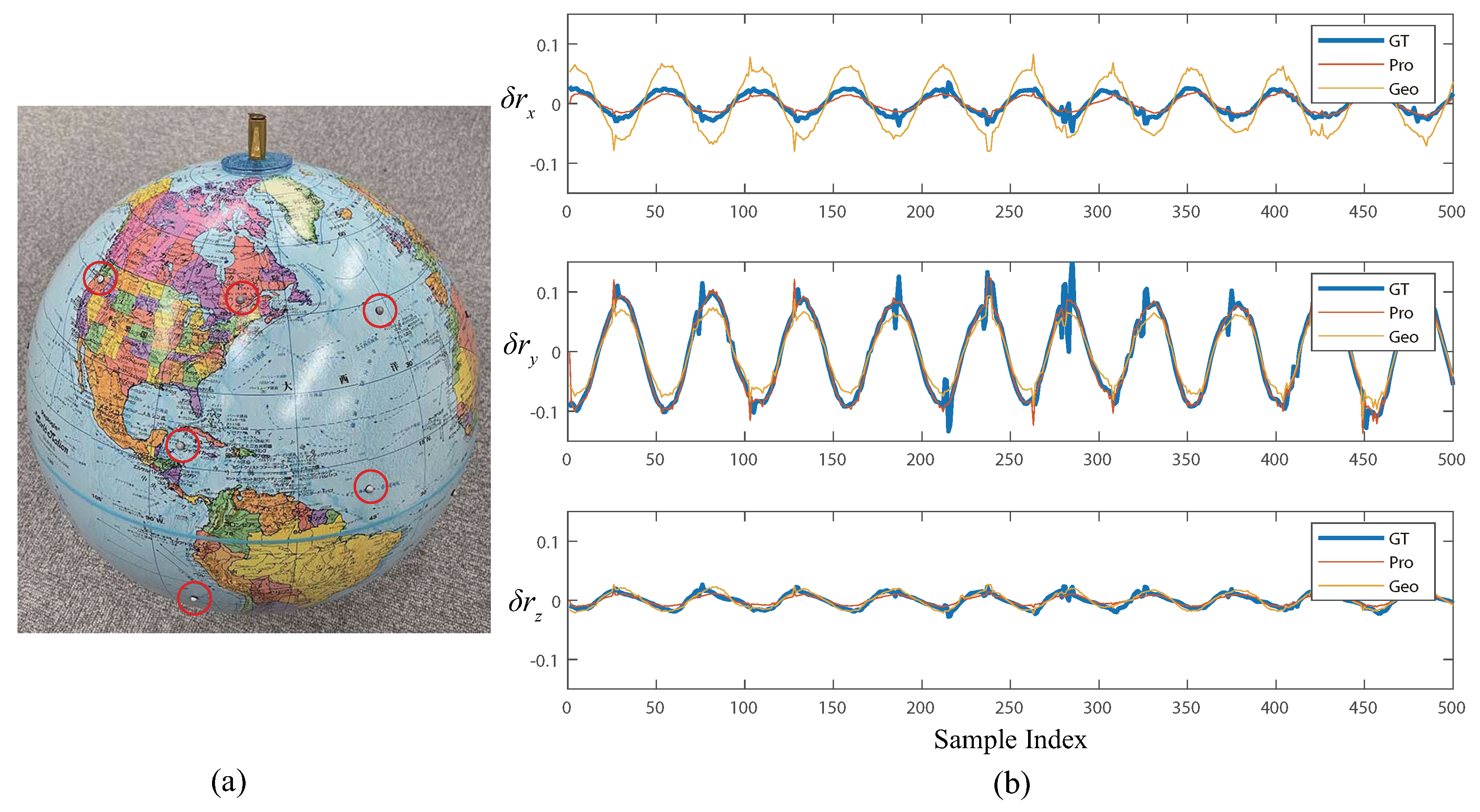
5.2. Sensing Daily Object
6. Conclusions
Author Contributions
Funding
Conflicts of Interest
References
- Hu, Y.; Miyashita, L.; Watanabe, Y.; Ishikawa, M. Robust 6-DOF motion sensing for an arbitrary rigid body by multi-view laser Doppler measurements. Opt. Express 2017, 25, 30371–30387. [Google Scholar] [CrossRef] [PubMed]
- Won, S.P.; Golnaraghi, F.; Melek, W.W. A Fastening Tool Tracking System Using an IMU and a Position Sensor With Kalman Filters and a Fuzzy Expert System. IEEE Trans. Ind. Electron. 2009, 56, 1782–1792. [Google Scholar] [CrossRef]
- Yi, C.; Ma, J.; Guo, H.; Han, J.; Gao, H.; Jiang, F.; Yang, C. Estimating Three-Dimensional Body Orientation Based on an Improved Complementary Filter for Human Motion Tracking. Sensors 2018, 18, 3765. [Google Scholar] [CrossRef] [PubMed]
- Besl, P.J.; McKay, N.D. A method for registration of 3-D shapes. IEEE Trans. Pattern Anal. Mach. Intell. 1992, 14, 239–256. [Google Scholar] [CrossRef]
- Chetverikov, D.; Svirko, D.; Stepanov, D.; Krsek, P. The Trimmed Iterative Closest Point algorithm. In Proceedings of the 16th International Conference on Pattern Recognition, Quebec City, QC, Canada, 11–15 August 2002; Volume 3, pp. 545–548. [Google Scholar] [CrossRef]
- Garon, M.; Lalonde, J. Deep 6-DOF Tracking. IEEE Trans. Vis. Comput. Gr. 2017, 23, 2410–2418. [Google Scholar] [CrossRef] [PubMed]
- Engel, J.; Koltun, V.; Cremers, D. Direct Sparse Odometry. IEEE Trans. Pattern Anal. Mach. Intell. 2018, 40, 611–625. [Google Scholar] [CrossRef] [PubMed]
- Hu, Y.; Miyashita, L.; Watanabe, Y.; Ishikawa, M. GLATUI: Non-intrusive Augmentation of Motion-based Interactions Using a GLDV. In Proceedings of the Extended Abstracts of the 2018 CHI Conference on Human Factors in Computing Systems (CHI E ’18), Montreal, QC, Canada, 21–26 April 2018; ACM: New York, NY, USA, 2018; pp. 1–6. [Google Scholar] [CrossRef]
- Vass, J.; Šmíd, R.; Randall, R.; Sovka, P.; Cristalli, C.; Torcianti, B. Avoidance of speckle noise in laser vibrometry by the use of kurtosis ratio: Application to mechanical fault diagnostics. Mech. Syst. Signal Process. 2008, 22, 647–671. [Google Scholar] [CrossRef]
- Rothberg, S. Numerical simulation of speckle noise in laser vibrometry. Appl. Opt. 2006, 45, 4523–4533. [Google Scholar] [CrossRef] [PubMed]
- Chang, Y.H.; Liu, C.S.; Cheng, C.C. Design and Characterisation of a Fast Steering Mirror Compensation System Based on Double Porro Prisms by a Screw-Ray Tracing Method. Sensors 2018, 18, 4046. [Google Scholar] [CrossRef] [PubMed]
- Liu, C.-S.; Lin, K.-W. Numerical and experimental characterization of reducing geometrical fluctuations of laser beam based on rotating optical diffuser. Opt. Eng. 2014, 53, 122408. [Google Scholar] [CrossRef]
- Sels, S.; Bogaerts, B.; Vanlanduit, S.; Penne, R. Extrinsic Calibration of a Laser Galvanometric Setup and a Range Camera. Sensors 2018, 18, 1478. [Google Scholar] [CrossRef] [PubMed]
- Tu, J.; Zhang, L. Effective Data-Driven Calibration for a Galvanometric Laser Scanning System Using Binocular Stereo Vision. Sensors 2018, 18, 197. [Google Scholar] [CrossRef] [PubMed]
- Wissel, T.; Wagner, B.; Stüber, P.; Schweikard, A.; Ernst, F. Data-Driven Learning for Calibrating Galvanometric Laser Scanners. IEEE Sens. J. 2015, 15, 5709–5717. [Google Scholar] [CrossRef]
- Quéau, Y.; Leporcq, F.; Alfalou, A. Design and simplified calibration of a Mueller imaging polarimeter for material classification. Opt. Lett. 2018, 43, 4941–4944. [Google Scholar] [CrossRef] [PubMed]
- Triggs, B.; McLauchlan, P.F.; Hartley, R.I.; Fitzgibbon, A.W. Bundle Adjustment—A Modern Synthesis. In Vision Algorithms: Theory and Practice; Triggs, B., Zisserman, A., Szeliski, R., Eds.; Springer: Berlin/Heidelberg, Germany, 2000; pp. 298–372. [Google Scholar]
- Vasconcelos, F.; Barreto, J.P.; Nunes, U. A Minimal Solution for the Extrinsic Calibration of a Camera and a Laser-Rangefinder. IEEE Trans. Pattern Anal. Mach. Intell. 2012, 34, 2097–2107. [Google Scholar] [CrossRef] [PubMed]
- Scaramuzza, D.; Harati, A.; Siegwart, R. Extrinsic self calibration of a camera and a 3D laser range finder from natural scenes. In Proceedings of the 2007 IEEE/RSJ International Conference on Intelligent Robots and Systems (IROS’07), San Diego, CA, USA, 29 October–2 November 2007; pp. 4164–4169. [Google Scholar]
- Lepetit, V.; Moreno-Noguer, F.; Fua, P. EPnP: An Accurate O(n) Solution to the PnP Problem. Int. J. Comput. Vis. 2008, 81, 155. [Google Scholar] [CrossRef]
- Trucco, E.; Verri, A. Introductory Techniques for 3-D Computer Vision; Prentice Hall: New Jersey, NJ, USA, 1998; Volume 201. [Google Scholar]
- Marquardt, D. An Algorithm for Least-Squares Estimation of Nonlinear Parameters. J. Soc. Ind. Appl. Math. 1963, 11, 431–441. [Google Scholar] [CrossRef]
- Zhang, Z. A flexible new technique for camera calibration. IEEE Trans. Pattern Anal. Mach. Intell. 2000, 22, 1330–1334. [Google Scholar] [CrossRef]
- Heikkila, J.; Silven, O. A four-step camera calibration procedure with implicit image correction. In Proceedings of the IEEE Computer Society Conference on Computer Vision and Pattern Recognition, San Juan, PR, USA, 17–19 June 1997; pp. 1106–1112. [Google Scholar] [CrossRef]
- Huber, P.J. Robust Estimation of a Location Parameter. Ann. Math. Stat. 1964, 35, 73–101. [Google Scholar] [CrossRef]


| Motion Pattern | ||||
|---|---|---|---|---|
| 0.0036 | 0.0012 | 0.280 | 0.2201 | |
| 0.0088 | 0.0424 | 0.501 | 3.39 | |
| 1.31 | 0 | 99.2 | 0 |
| Test Set | Rotational (Rad) | Translational (mm) | ||
|---|---|---|---|---|
| Proposed | Geo | Proposed | Geo | |
| 0.0139 | 0.0484 | 2.3142 | 9.0864 | |
| 0.0108 | 0.0321 | 2.0543 | 4.9750 | |
| 0.0239 | 0.0321 | 3.8263 | 7.6578 | |
| 0.0101 | 0.0089 | 3.1751 | 3.4187 | |
| 0.0077 | 0.0220 | 1.9044 | 3.8176 | |
| 0.0054 | 0.0075 | 1.6014 | 2.7850 | |
| 0.0133 | 0.0290 | 2.5977 | 5.7731 | |
© 2019 by the authors. Licensee MDPI, Basel, Switzerland. This article is an open access article distributed under the terms and conditions of the Creative Commons Attribution (CC BY) license (http://creativecommons.org/licenses/by/4.0/).
Share and Cite
Hu, Y.; Miyashita, L.; Watanabe, Y.; Ishikawa, M. Visual Calibration for Multiview Laser Doppler Speed Sensing. Sensors 2019, 19, 582. https://doi.org/10.3390/s19030582
Hu Y, Miyashita L, Watanabe Y, Ishikawa M. Visual Calibration for Multiview Laser Doppler Speed Sensing. Sensors. 2019; 19(3):582. https://doi.org/10.3390/s19030582
Chicago/Turabian StyleHu, Yunpu, Leo Miyashita, Yoshihiro Watanabe, and Masatoshi Ishikawa. 2019. "Visual Calibration for Multiview Laser Doppler Speed Sensing" Sensors 19, no. 3: 582. https://doi.org/10.3390/s19030582
APA StyleHu, Y., Miyashita, L., Watanabe, Y., & Ishikawa, M. (2019). Visual Calibration for Multiview Laser Doppler Speed Sensing. Sensors, 19(3), 582. https://doi.org/10.3390/s19030582