A Spatial Adaptive Algorithm Framework for Building Pattern Recognition Using Graph Convolutional Networks


Abstract
1. Introduction
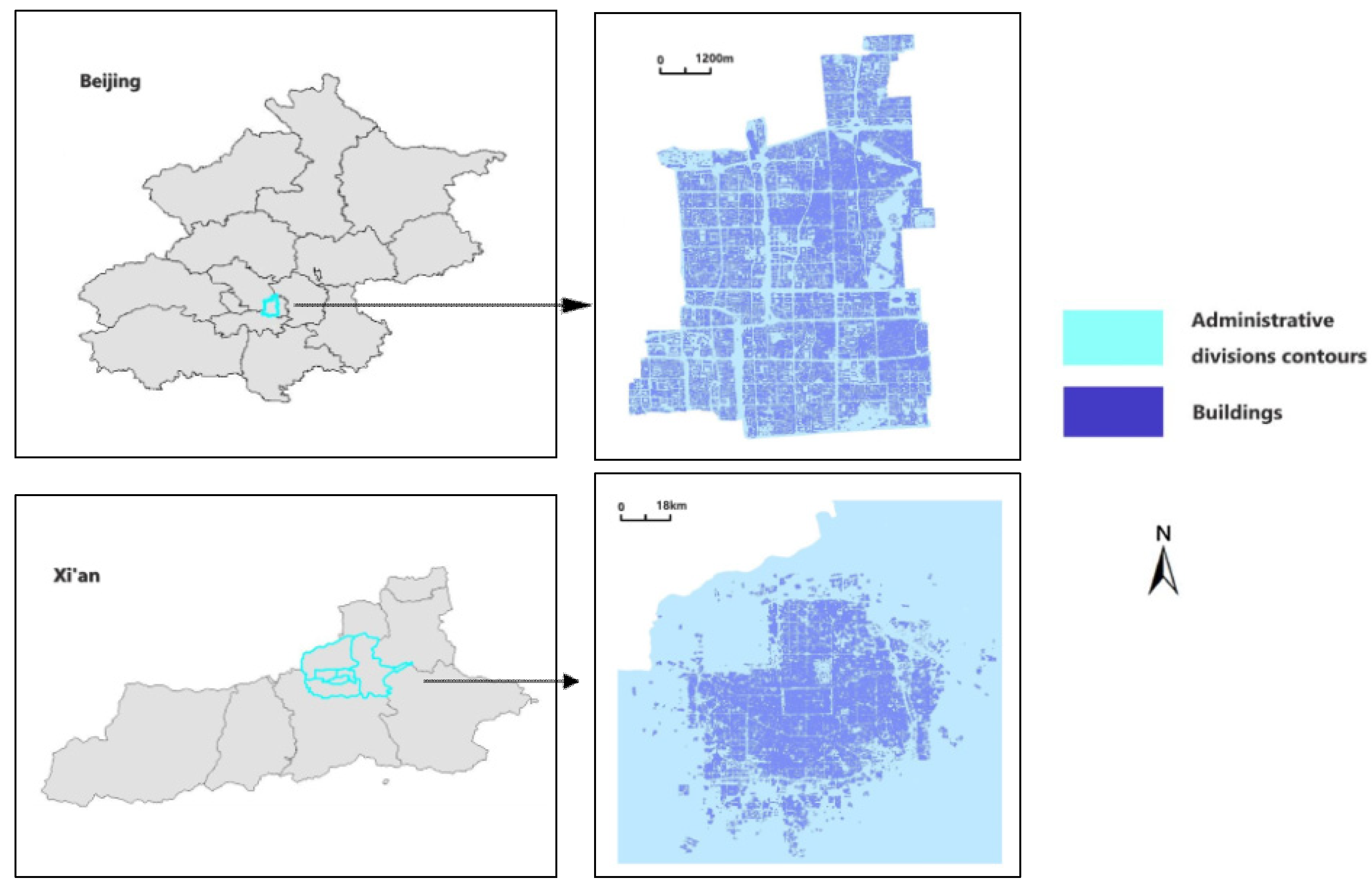
2. Study Materials
3. Methodology
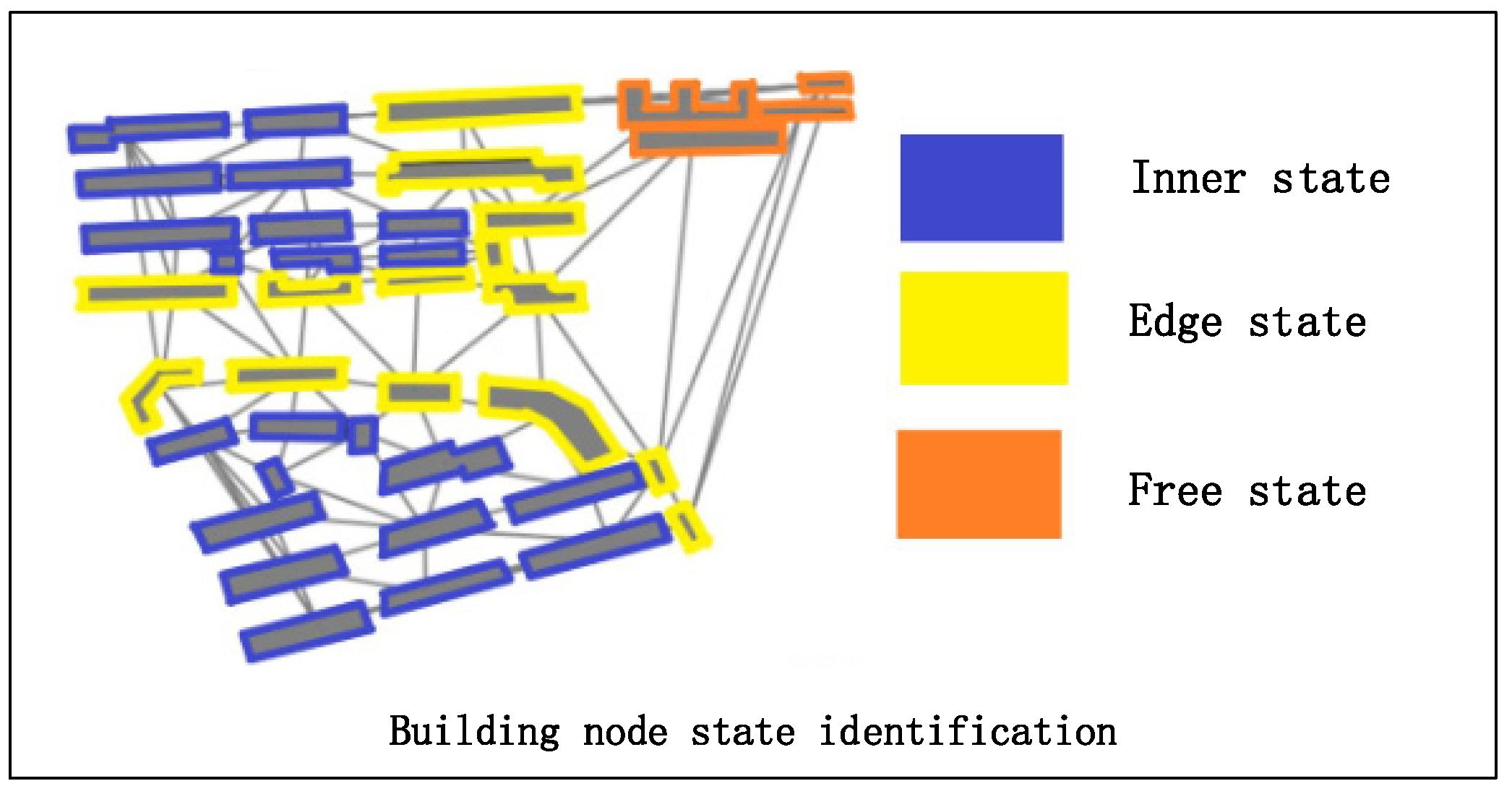
3.1. Building Node State Identification
3.1.1. Definition of Three Building Node States
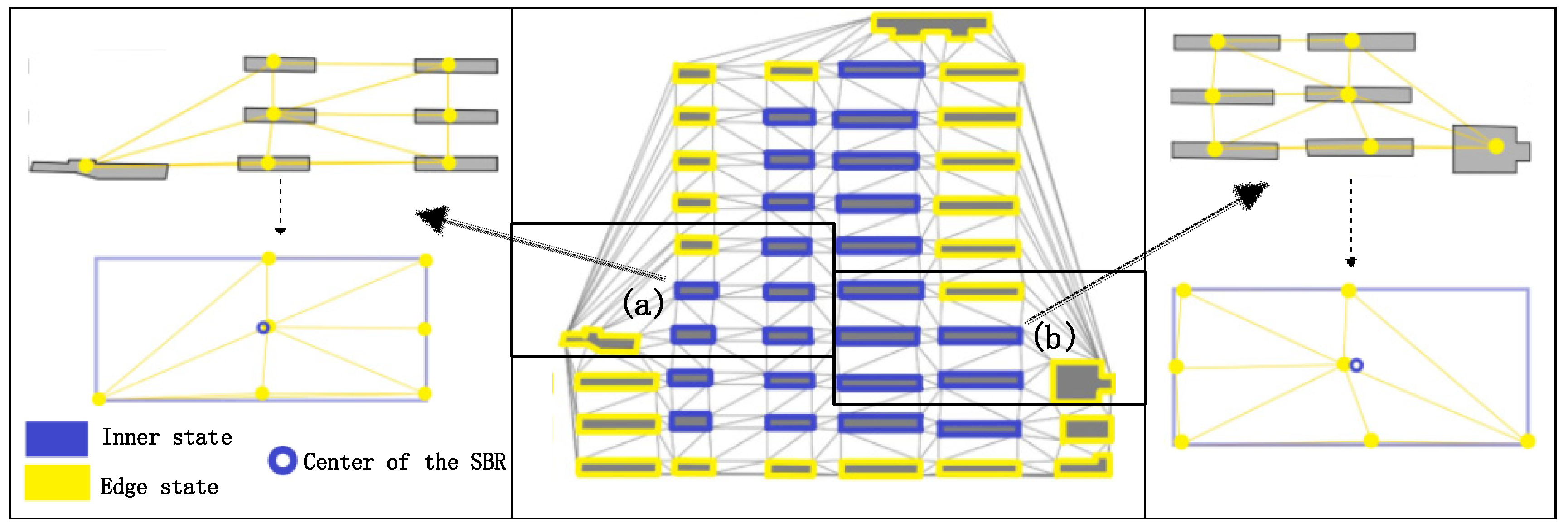
- Edge state. Intuitively, the edge state buildings are located on the edge of a building block. Their unique characteristic is that the contrast between the buildings of their two sides is strong (e.g., the bright yellow buildings shown in Figure 2). The contrast embodied by the difference of the descriptive vectors of building nodes will lead to unique feature encoding through the graph convolution operation. Therefore, the definition of edge state is reasonable, and it is indicative of the inner state building.
- Inner state. Buildings located in the same building pattern are similar in terms of size, outline and spatial position; hence, buildings located in the same pattern are defined as the inner state buildings (e.g., the blue buildings shown in Figure 2).
- Free state. Normally, there is one building that exhibits independence because of its spatial distance among others. We define such buildings as free state buildings (e.g., the orange buildings shown in Figure 2).
3.1.2. Descriptive Methods for Building Features
3.1.2.1. Definition of the Shifting Degree of Adjacency Weight
3.1.2.2. Description for Building Orientation
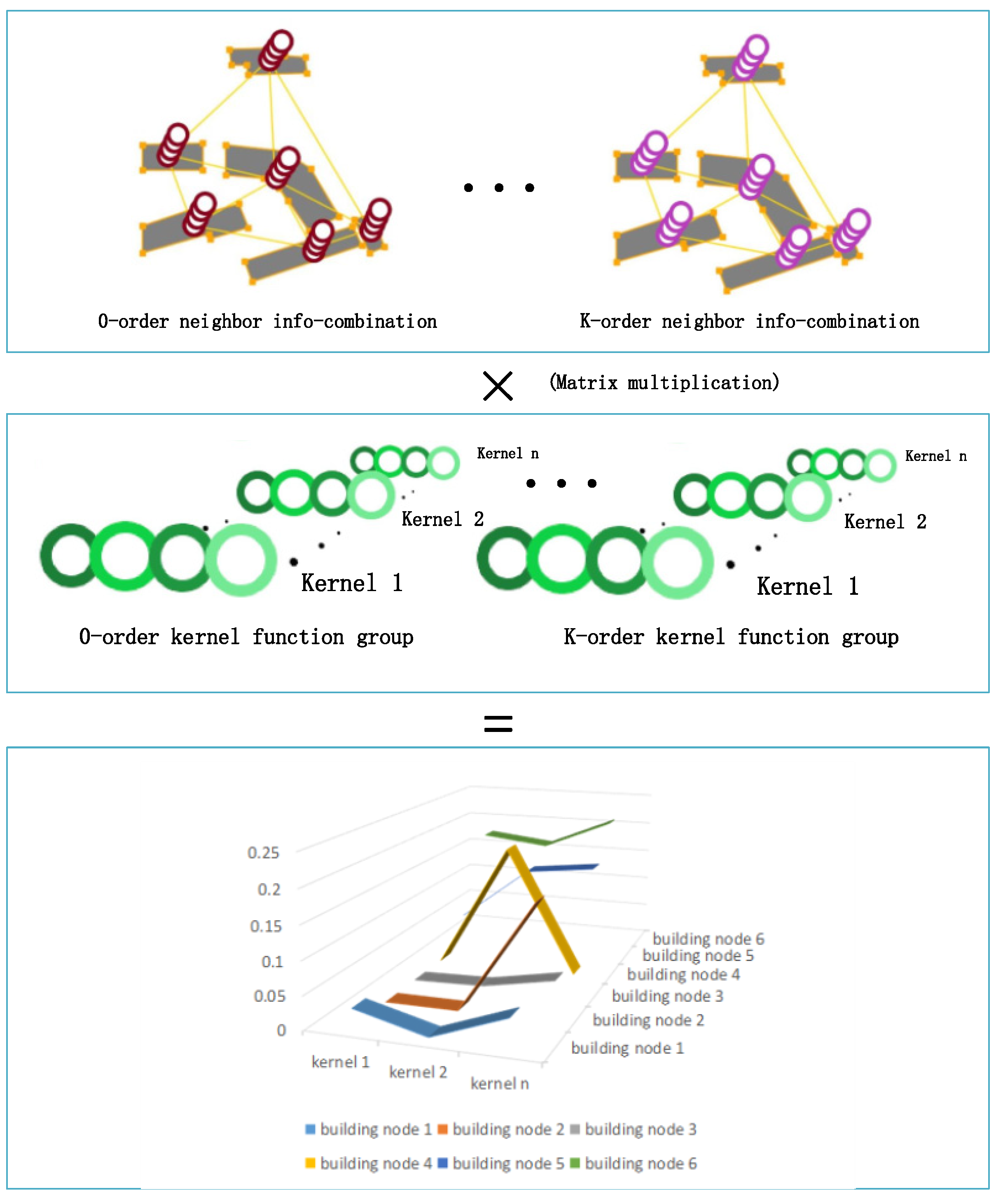
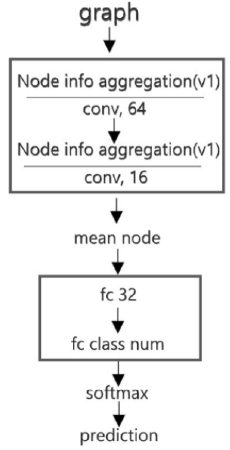
3.1.3. Graph Convolutional Network
- Aggregating the differences between each building and its Kth-order neighbors based on adjacency information;
- Realizing local weight sharing for the convolutional kernels, and;
- Reducing the computational cost for learning.
| Algorithm 1 BFS (G, , , ) |
| 1: Initialize: (an empty stack for the BFS algorithm). 2: push to 3: while not empty () do 4: ← 5: = neighbors () 6: for each do 7: if ’s state is then 8: append to 9: push to 10: Return: |
| Algorithm 2 Inner state node searching process for group pattern reconstruction |
| 1: Input: Building graph G = (V, E) (where V[i] stores the state of building i recognized by the GCN (Section 3.1.3)); number of building nodes = N 2: Initialize: (an empty list to store the building groups of inner state), = 0 3: for i = 0 to N − 1 do 4: if V[i] is state and have not been appended to then 5: , append(V[i]) to 6: BFS (G, , V[i], state) ◁BFS(Algorithm 1) for node traversing 7: for i = 0 to N − 1 do 8: if V[i] is state and have not been appended to then 9: for j = 0 to − 1 do 10: for k = 0 to − 1 do 11: if V[i] and is state then 12: append(V[i]) to 13: Return: |
| Algorithm 3 Edge state node searching process for group pattern reconstruction |
| 1: Input: Building graph G = (V, E) (where V[i] stores the state of building i recognized by the GCN (Section 3.1.3)); number of building nodes = N 2: Initialize: (an empty list to store building groups of edge state), = 0 3: for i = 0 to N − 1 do 4: if V[i] is state and have not been appended to or then 5: , append(V[i]) to 6: BFS (G, , V[i], state) ◁BFS(Algorithm 1) for node traversing 7: Return: |
| Algorithm 4 Free state node searching process for group pattern reconstruction |
| 1: Input: Building graph G = (V, E) (where V[i] stores the state of building i recognized by the GCN (Section 3.1.3)); number of building nodes = N 2: Initialize: (an empty list to store the building groups of free state), = 0 3: for i = 0 to N − 1 do 4: if V[i] is state and have not been appended to then 5: , append(V[i]) to 6: BFS (G, , V[i], state) ◁BFS(Algorithm 1) for node traversing 7: Return: |
3.2. Building Group Partition Algorithm
- Situations of inner state: There is only one existing situation of inner state nodes in a building block. As shown in Figure 9b, the inner state nodes are surrounded by the edge state nodes, and form the building block with the latter. Algorithm 2 is used for obtaining the building block containing inner state nodes.
- Situations of edge state nodes: As shown in Figure 9b,e there are two possible situations of edge state nodes: 1. forming the building block with inner state nodes and 2. forming the building block only consisting of edge state nodes. Algorithm 2 is adapted to the first situation, while Algorithm 3 is applied to the second situation.
- Situations of free state nodes: There is only one possible situation of free state nodes because of its independence compared to the other two kinds of building nodes, as shown in Figure 9c. Algorithm 4 is used for constructing the building group consisting only of free state nodes.
- Building nodes in the same state, but not in the same building block: It is possible that, though the nodes are identified as nodes in the same state, they belong to different building blocks (Figure 9d). Moreover, a fine-grained partition is needed because of the differences in the aspects of size, outline and orientation because the group partition step mainly focuses on the spatial distribution. This problem will be solved in the following step.
| Algorithm 5 Building node clustering |
| 1: Input: Building graph G = (V, E) (where ∈ V means the building nodes from the same building division (Section 3.2)); N means the number of buildings 2: Initialize: (an empty list to store building pattern groups), M (a list initialized by False, storing the state if have been checked), (an empty stack for the BFS algorithm), RF (a function using the RF model to judge whether the buildings should be in the same pattern; see Section 3.3), L = N, = 1 3: while L > 0 do 4: L --, ++, T ← None 5: append () to , push to ◁ where V and M[i] == False 6: while not empty () do 7: ← , M ← True 8: = neighbors () 9: sort ◁ by the distances to in ascending order 10: for each do 11: if T == None and M[ ] == False then 12: if RF , is True then 13: T ← , append to , push to , L -- 14: else if and M == False then 15: if RF , , T is True then 16: append to , push to , L -- 17: Return: |
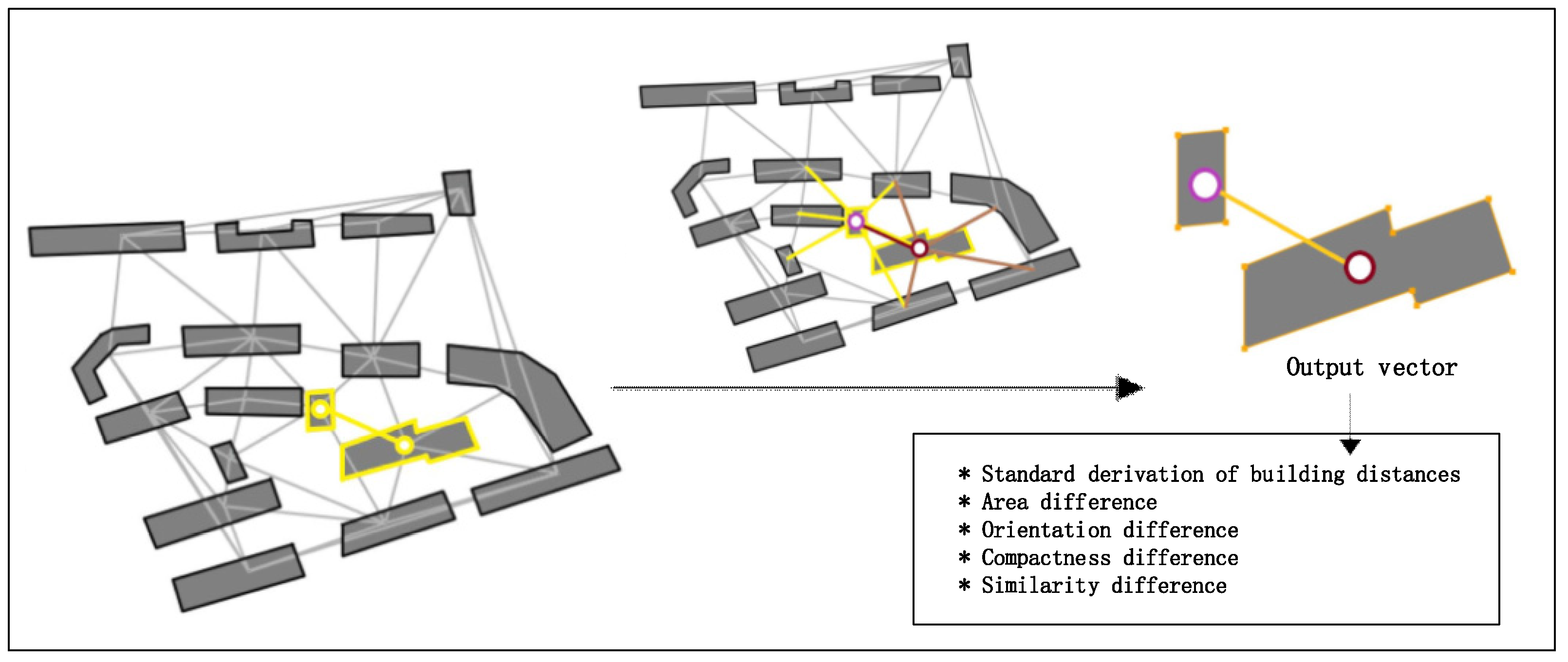
3.3. Fine-Grained Partition for Building Blocks
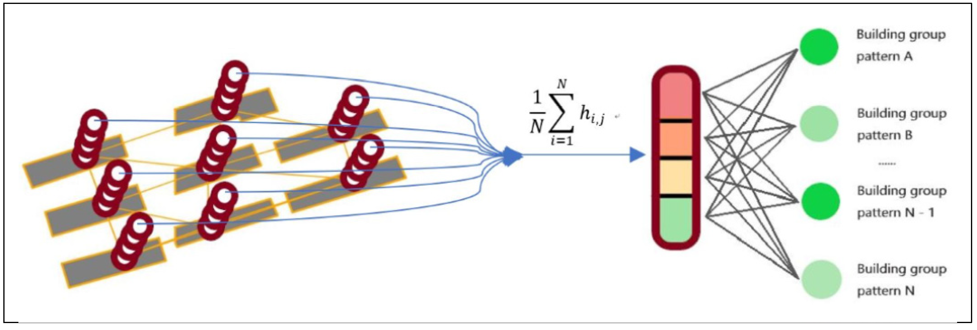
3.4. Building Pattern Recognition
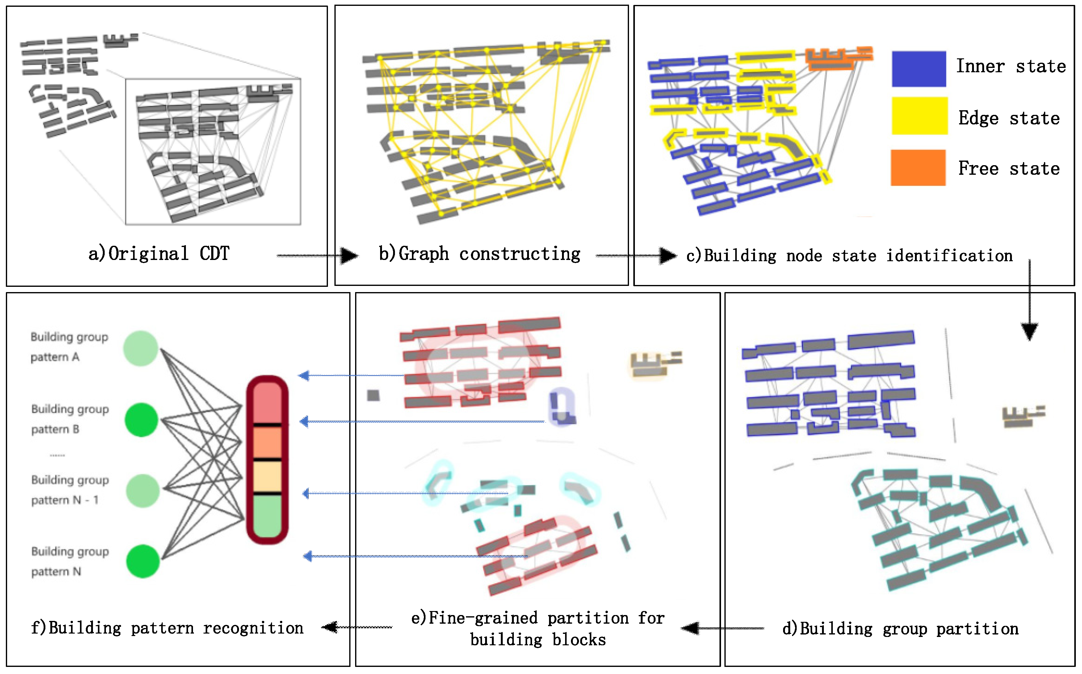
4. Framework for Building Pattern Recognition
- Building node state identification. Based on the vector data of building contours, each building entity is described by indices including its area, perimeter, orientation, compactness and shifting degree of adjacency weight (Section 3.1.2.1), and then a descriptive vector is constructed. The descriptive vectors are the input to the GCN model in the subsequent step. To make rules for building group partition, three states (edge state, inner state and free state) (Section 3.1.1) are defined to describe the spatial state of the buildings. The related dataset of building node state labeling is constructed, and the GCN model with semi-supervised learning is trained to enhance the ability of generalization. The GCN model is used to identify the building node state, which is indispensable for the building group partition algorithm (see Section 3.2). The partition process and the building samples identified as different states are shown in Figure 12c.
- Building group partitioning. The building group partition algorithm based on the identification results of the building state is run. The outputs of the algorithm are the building blocks from the partitioned building groups (Figure 12d).
- Building node clustering. A breadth-first search (BFS) is used to traverse building nodes in a graph, and the graph of each building block is constructed by CDT. A random forest (RF) algorithm is introduced to judge whether two or three building entities (Section 3.3) can be categorized into the same building pattern. The objective of this step is to extract all the separate building patterns in a building block (Figure 12e).
- Building pattern recognition. In this final step, a GCNN model (Section 3.4) is used to recognize the building patterns, as shown in Figure 12f. The model is trained with supervised learning with the building node pattern datasets.
| Algorithm 6 Framework for building pattern recognition |
| 1: Require: 2: X: denotes the data of a building block selected in advance. 3: Xj: denotes primary data of a building object with ID j, including the coordinate data of 4: the building contours. 5: Step 1: Construct a graph G for X using CDT. 6: Step 2: Calculate the values of the variables mentioned in Section 3.1.2 to construct a 7: new descriptive vector for each building object , on the basis of the adjacent relations 8: derived from the graph G. 9: Step 3: Classify each building Xj into the state Sj by the GCN model (see Section 3.1.3). 10: Step 4: Accomplish building graph partition. Functions , and 11: stand for Algorithms 2–4 respectively. 12: = 13: = 14: 15: Where [i] denotes the building group and [i] = [ … ]. stands for 16: the number of the buildings of the building group. Data structures of and 17: are the same as . 18: Step 5: Utilize the RF model to accomplish the fine-grained partition (Section 3.3) for 19: the building groups from , and . 20: Initialize: 21: Sl: an empty list. 22: : a list consists of all the building groups from , and . 22: for i = 0 to − 1 do 23: = [i] 24: = ◁ stands for the function of Algorithm 5 25: for j = 0 to − 1 do 26: append to ◁ denotes a building group 27: end for 28: end for 29: Step 6: Classify the building group into the pattern with the GCNN model. 30: for i = 0 to − 1 do 31: = ◁ means the classifying result 32: end for |
5. Experiments and Results
5.1. Building Node State Recognition
5.2. Fine-Grained Partition
5.3. Building Group Pattern Recognition and Comparative Analysis
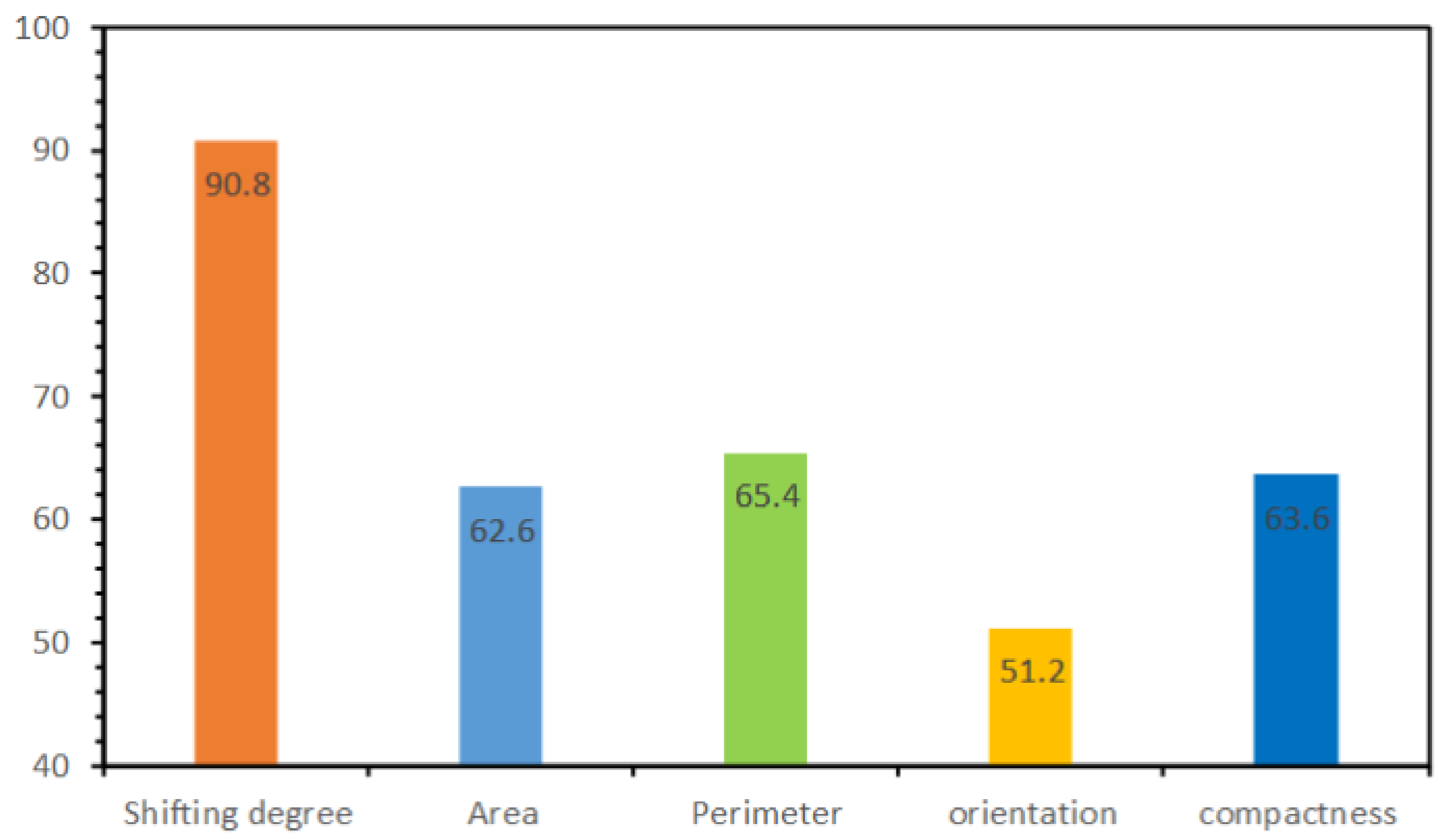
5.4. Parameter Descriptive Ability Analysis
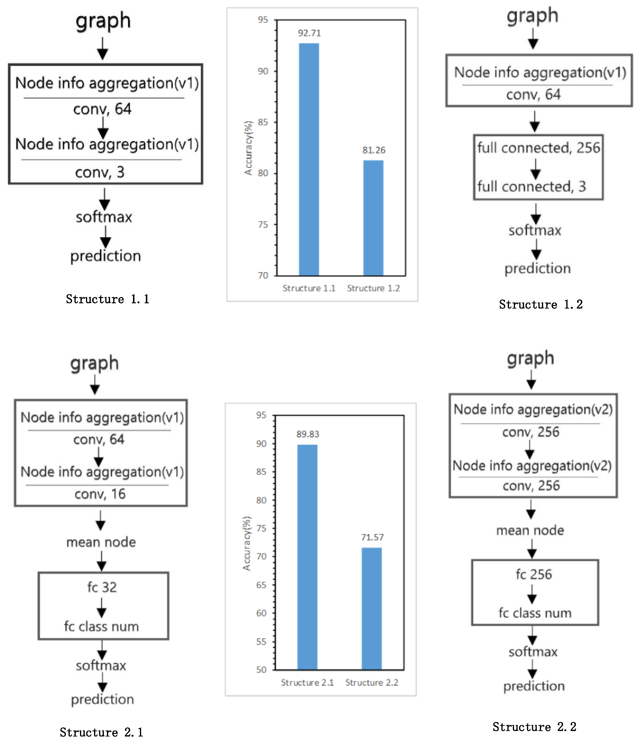
5.5. Model Structure Exploration Results
6. Discussion
6.1. Spatial Adaptive Algorithm Framework Using GCNs
6.2. Remaining Issues
7. Conclusions and Future Works
7.1. Conclusions
7.2. Future Works
Author Contributions
Funding
Conflicts of Interest
References
- Du, S.; Luo, L.; Cao, K.; Shu, M. Extracting building patterns with multilevel graph partition and building grouping. ISPRS J. Photogramm. Remote Sens. 2016, 122, 81–96. [Google Scholar] [CrossRef]
- Du, S.; Shu, M.; Feng, C. Representation and discovery of building patterns: A three-level relational approach. Int. J. Geogr. Inf. Sci. 2016, 30, 1161–1186. [Google Scholar] [CrossRef]
- Yan, X.; Ai, T.; Yang, M.; Yin, H. A graph convolutional neural network for classification of building patterns using spatial vector data. ISPRS J. Photogramm. Remote Sens. 2019, 150, 259–273. [Google Scholar] [CrossRef]
- He, X.; Zhang, X.; Xin, Q. Recognition of building group patterns in topographic maps based on graph partitioning and random forest. ISPRS J. Photogramm. Remote Sens. 2018, 136, 26–40. [Google Scholar] [CrossRef]
- Regnauld, N. Contextual Building Typification in Automated Map Generalization. Algorithmica 2001, 30, 312–333. [Google Scholar] [CrossRef]
- Li, Z.; Yan, H.; Ai, T.; Chen, J. Automated building generalization based on urban morphology and Gestalt theory. Int. J. Geogr. Inf. Sci. 2004, 18, 513–534. [Google Scholar] [CrossRef]
- Deng, M.; Tang, J.; Liu, Q.; Wu, F. Recognizing building groups for generalization: A comparative study. Cartogr. Geogr. Inf. Sci. 2018, 45, 187–204. [Google Scholar] [CrossRef]
- Gonzalez-Abraham, C.E.; Radeloff, V.C.; Hammer, R.B.; Hawbaker, T.J.; Stewart, S.I.; Clayton, M.K. Building patterns and landscape fragmentation in northern Wisconsin, USA. Landsc. Ecol. 2007, 22, 217–230. [Google Scholar] [CrossRef]
- Girshick, R. Fast R-CNN. In Proceedings of the IEEE International Conference on Computer Vision (ICCV), Santiago, Chile, 13–16 December 2015; pp. 1440–1448. [Google Scholar]
- Ren, S.; He, K.; Girshick, R.; Sun, J. Faster R-CNN: Towards Real-Time Object Detection with Region Proposal Networks. In Advances in Neural Information Processing Systems 28; Cortes, C., Lawrence, N.D., Lee, D.D., Sugiyama, M., Garnett, R., Eds.; Curran Associates, Inc.: Montreal, QC, Canada, 2015; pp. 91–99. [Google Scholar]
- Redmon, J.; Divvala, S.; Girshick, R.; Farhadi, A. You Only Look Once: Unified, Real-Time Object Detection. In Proceedings of the IEEE Conference on Computer Vision and Pattern Recognition (CVPR), Las Vegas, NV, USA, 26 June 2016; pp. 779–788. [Google Scholar]
- Girshick, R.; Donahue, J.; Darrell, T.; Malik, J. Rich Feature Hierarchies for Accurate Object Detection and Semantic Segmentation. In Proceedings of the IEEE Conference on Computer Vision and Pattern Recognition (CVPR), Columbus, OH, USA, 24–27 June 2014; pp. 580–587. [Google Scholar]
- He, K.; Gkioxari, G.; Dollar, P.; Girshick, R. Mask R-CNN. In Proceedings of the IEEE International Conference on Computer Vision (ICCV), Venice, Italy, 22–29 October 2017; pp. 2961–2969. [Google Scholar]
- Long, J.; Shelhamer, E.; Darrell, T. Fully Convolutional Networks for Semantic Segmentation. In Proceedings of the IEEE Conference on Computer Vision and Pattern Recognition (CVPR), Boston, MA, USA, 7–12 June 2015; pp. 91–99. [Google Scholar]
- Kipf, T.N.; Welling, M. Semi-Supervised Classification with Graph Convolutional Networks. arXiv 2016, arXiv:1609.02907. [Google Scholar]
- Fout, A.; Byrd, J.; Shariat, B.; Ben-Hur, A. Protein Interface Prediction using Graph Convolutional Networks. In Advances in Neural Information Processing Systems 30; Guyon, I., Luxburg, U.V., Bengio, S., Wallach, H., Fergus, R., Vishwanathan, S., Garnett, R., Eds.; Curran Associates, Inc.: Long Beach, CA, USA, 2017; pp. 6530–6539. [Google Scholar]
- Parisot, S.; Ktena, S.I.; Ferrante, E.; Lee, M.; Guerrero, R.; Glocker, B.; Rueckert, D. Disease prediction using graph convolutional networks: Application to Autism Spectrum Disorder and Alzheimer’s disease. Med. Image Anal. 2018, 48, 117–130. [Google Scholar] [CrossRef]
- Ping, X.; Shuxiang, P.; Tiangang, Z.; Yong, L.; Hao, S. Graph Convolutional Network and Convolutional Neural Network Based Method for Predicting lncRNA-Disease Associations. Cells 2019, 8, 1012. [Google Scholar]
- Fei, M.; Fei, G.; Jinping, S.; Huiyu, Z.; Amir, H. Attention Graph Convolution Network for Image Segmentation in Big SAR Imagery Data. Remote Sens. 2019, 11, 2586. [Google Scholar]
- Anselin, L. Local Indicators of Spatial Association—LISA. Geogr. Anal. 1995, 27, 93–115. [Google Scholar] [CrossRef]
- Tobler, W.R. A Computer Movie Simulating Urban Growth in the Detroit Region. Econ. Geogr. 1970, 46, 234–240. [Google Scholar] [CrossRef]
- Zhang, X.; Ai, T.; Stoter, J.; Kraak, M.; Molenaar, M. Building pattern recognition in topographic data: Examples on collinear and curvilinear alignments. Geoinformatica 2013, 17, 1–33. [Google Scholar] [CrossRef]
- Hamilton, W.; Ying, Z.; Leskovec, J. Inductive Representation Learning on Large Graphs. In Advances in Neural Information Processing Systems 30; Guyon, I., Luxburg, U.V., Bengio, S., Wallach, H., Fergus, R., Vishwanathan, S., Garnett, R., Eds.; Curran Associates, Inc.: Long Beach, CA, USA, 2017; pp. 1024–1034. [Google Scholar]
- Gou, J.; Qiu, W.; Yi, Z.; Xu, Y.; Mao, Q.; Zhan, Y. A Local Mean Representation-based K-Nearest Neighbor Classifier. ACM Trans. Intell. Syst. Technol. 2019, 10, 21–29. [Google Scholar] [CrossRef]
- Gou, J.; Wang, L.; Hou, B.; Lv, J.; Yuan, Y.; Mao, Q. Two-phase probabilistic collaborative representation-based classification. Expert Syst. Appl. 2019, 133, 9–20. [Google Scholar] [CrossRef]
- Gou, J.; Hou, B.; Yuan, Y.; Ou, W.; Zeng, S. A new discriminative collaborative representation-based classification method via l2 regularizations. Neural Comput. Appl. 2019, 1–15. [Google Scholar] [CrossRef]
- Chen, Y.N. Multiple Kernel Feature Line Embedding for Hyperspectral Image Classification. Remote Sens. 2019, 11, 2892. [Google Scholar] [CrossRef]
- Perozzi, B.; Al-Rfou, R.; Skiena, S. DeepWalk: Online Learning of Social Representations. In Proceedings of the 20th ACM SIGKDD International Conference on Knowledge Discovery and Data Mining, New York, NY, USA, 24–27 August 2014; pp. 701–710. [Google Scholar]
- Grover, A.; Leskovec, J. Node2Vec: Scalable Feature Learning for Networks. In Proceedings of the 22nd ACM SIGKDD International Conference on Knowledge Discovery and Data Mining, San Francisco, CA, USA, 13–17 August 2016; pp. 855–864. [Google Scholar]
- Tang, J.; Qu, M.; Wang, M.; Zhang, M.; Yan, J.; Mei, Q. LINE: Large-scale Information Network Embedding. In Proceedings of the 24th International Conference on World Wide Web, Florence, Italy, 18–22 May 2015; pp. 1067–1077. [Google Scholar]
- Wang, D.; Cui, P.; Zhu, W. Structural Deep Network Embedding. In Proceedings of the 22nd ACM SIGKDD International Conference on Knowledge Discovery and Data Mining, ACM, San Francisco, CA, USA, 13–17 August 2016; pp. 1225–1234. [Google Scholar]
- Defferrard, M.; Bresson, X.; Vandergheynst, P. Convolutional Neural Networks on Graphs with Fast Localized Spectral Filtering. In Advances in Neural Information Processing Systems 29; Lee, D.D., Sugiyama, M., Luxburg, U.V., Guyon, I., Garnett, R., Eds.; Curran Associates, Inc.: Barcelona, Spain, 2016; pp. 3844–3852. [Google Scholar]
- Babyak, M.A. What you see may not be what you get: A brief, nontechnical introduction to overfitting in regression-type models. Psychosom. Med. 2004, 66, 411–421. [Google Scholar]
- Hammond, D.K.; Vandergheynst, P.; Gribonval, R. Wavelets on graphs via spectral graph theory. Appl. Comput. Harmon. A 2011, 30, 129–150. [Google Scholar] [CrossRef]
- Scarselli, F.; Gori, M.; Tsoi, A.C.; Hagenbuchner, M.; Monfardini, G. The Graph Neural Network Model. IEEE Trans. Neural Netw. 2009, 20, 61–80. [Google Scholar] [CrossRef] [PubMed]
- Duvenaud, D.K.; Maclaurin, D.; Iparraguirre, J.; Bombarell, R.; Hirzel, T.; Aspuru-Guzik, A.; Adams, R.P. Convolutional Networks on Graphs for Learning Molecular Fingerprints. In Advances in Neural Information Processing Systems 28; Cortes, C., Lawrence, N.D., Lee, D.D., Sugiyama, M., Garnett, R., Eds.; Curran Associates, Inc.: Montreal, QC, Canada, 2015; pp. 2224–2232. [Google Scholar]
- Basaraner, M.; Cetinkaya, S. Performance of shape indices and classification schemes for characterising perceptual shape complexity of building footprints in GIS. Int. J. Geogr. Inf. Sci. 2017, 31, 1952–1977. [Google Scholar] [CrossRef]
- Peura, M.; Iivarinen, J. Efficiency of Simple Shape Descriptors. In Advances in Visual form Analysis: Proceedings of the 3rd International Workshop on Visual Form; World Scientific: Capri, Italy, 1997; pp. 443–451. [Google Scholar]
- LeCun, Y.; Bottou, L.; Bengio, Y.; Haffner, P. Gradient-Based Learning Applied to Document Recognition. Proc. IEEE 1998, 86, 2278–2324. [Google Scholar] [CrossRef]
- Gilmer, J.; Schoenholz, S.S.; Riley, P.F.; Vinyals, O.; Dahl, G.E. Neural Message Passing for Quantum Chemistry. In Proceedings of the 34th International Conference on Machine Learning, JMLR.org, Sydney, NSW, Australia, 6–11 August 2017; pp. 1263–1272. [Google Scholar]
- Jones, C.B.; Bundy, G.L.; Ware, M.J. Map Generalization with a Triangulated Data Structure. Am. Cartogr. 1999, 22, 317–331. [Google Scholar]
- Touya, G.; Coupé, A.; Jollec, J.L.; Dorie, O.; Fuchs, F. Conflation Optimized by Least Squares to Maintain Geographic Shapes. ISPRS Int. J. Geo-Inf. 2013, 2, 621–644. [Google Scholar] [CrossRef]
- Zhang, X.; Ai, T.; Stoter, J. Characterization and Detection of Building Patterns in Cartographic Data: Two Algorithms. In Advances in Spatial Data Handling and GIS; Springer: Berlin/Heidelberg, Germany, 2012; pp. 93–107. [Google Scholar]


| Variable | Index | Equation | Description |
|---|---|---|---|
| Position feature | Shifting degree of adjacency weight in width direction | - | See Section 3.1.2.1 |
| Shifting degree of adjacency weight in height direction | - | See Section 3.1.2.1 | |
| Size | Area index | Building area with normalizing operation Building perimeter with normalizing operation | |
| Perimeter index | |||
| Orientation | Orientation index | - | See Section 3.1.2.2 |
| Shape | Compactness | Quadratic relationship between the area and the perimeter [37] | |
| Concavity | Area ratio of the building to its convex hull [37] |
| Number of Examples = 950 | Actual Inner State | Actual Edge State | Actual Free State |
|---|---|---|---|
| Predicted inner state | 668 | 24 | 1 |
| Predicted edge state | 37 | 184 | 2 |
| Predicted free state | 0 | 0 | 34 |
| Method | Training Accuracy (Beijing Xicheng District) | Testing Accuracy (Xi’an) |
|---|---|---|
| SVM | 98.30% | 84.35% |
| RF | 99.06% | 96.77% |
| Method | Training Accuracy (Beijing Xicheng District) | Testing Accuracy (Xi’an) |
|---|---|---|
| SVM | 99.68% | 77.18% |
| RF | 99.45% | 81.78% |
| GCNN | 98.20% | 89.83% |
| Number of Examples = 354 | Actual I-Shape | Actual L-Shape | Actual Grid-Like |
|---|---|---|---|
| Predicted I-shape | 118 | 9 | 11 |
| Predicted L-shape | 6 | 109 | 7 |
| Predicted Grid-like | 1 | 2 | 91 |
| Method | Training Accuracy (Beijing Xicheng District) | Testing Accuracy (Xi’an) |
|---|---|---|
| SVM | 94.52% | 81.35% |
| RF | 96.84% | 89.39% |
| GCNN | 86.05% | 92.71% |
© 2019 by the authors. Licensee MDPI, Basel, Switzerland. This article is an open access article distributed under the terms and conditions of the Creative Commons Attribution (CC BY) license (http://creativecommons.org/licenses/by/4.0/).
Share and Cite
Bei, W.; Guo, M.; Huang, Y. A Spatial Adaptive Algorithm Framework for Building Pattern Recognition Using Graph Convolutional Networks. Sensors 2019, 19, 5518. https://doi.org/10.3390/s19245518
Bei W, Guo M, Huang Y. A Spatial Adaptive Algorithm Framework for Building Pattern Recognition Using Graph Convolutional Networks. Sensors. 2019; 19(24):5518. https://doi.org/10.3390/s19245518
Chicago/Turabian StyleBei, Weijia, Mingqiang Guo, and Ying Huang. 2019. "A Spatial Adaptive Algorithm Framework for Building Pattern Recognition Using Graph Convolutional Networks" Sensors 19, no. 24: 5518. https://doi.org/10.3390/s19245518
APA StyleBei, W., Guo, M., & Huang, Y. (2019). A Spatial Adaptive Algorithm Framework for Building Pattern Recognition Using Graph Convolutional Networks. Sensors, 19(24), 5518. https://doi.org/10.3390/s19245518