Figure 1.
The wearable device for sensing photoplethysmogram (PPG) signals and the mobile application for PPG, photoplethysmogram (GPS), ambient noise, and self-report data acquisition.
Figure 1.
The wearable device for sensing photoplethysmogram (PPG) signals and the mobile application for PPG, photoplethysmogram (GPS), ambient noise, and self-report data acquisition.
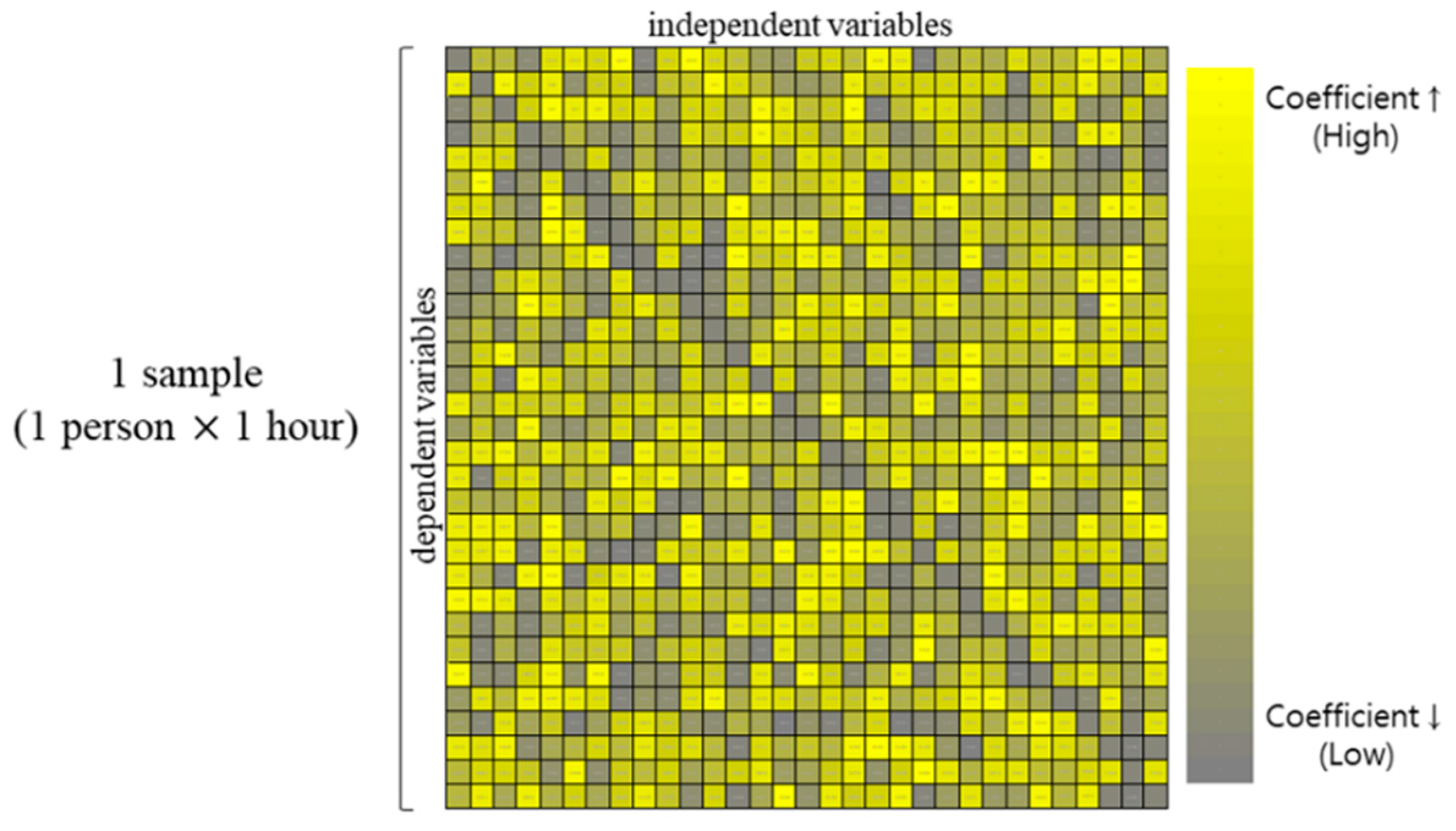
Figure 2.
A sample of standardized coefficient matrix. The standardized coefficient which is beta (β) indicates the influence of each independent variable on the dependent variable.
Figure 2.
A sample of standardized coefficient matrix. The standardized coefficient which is beta (β) indicates the influence of each independent variable on the dependent variable.
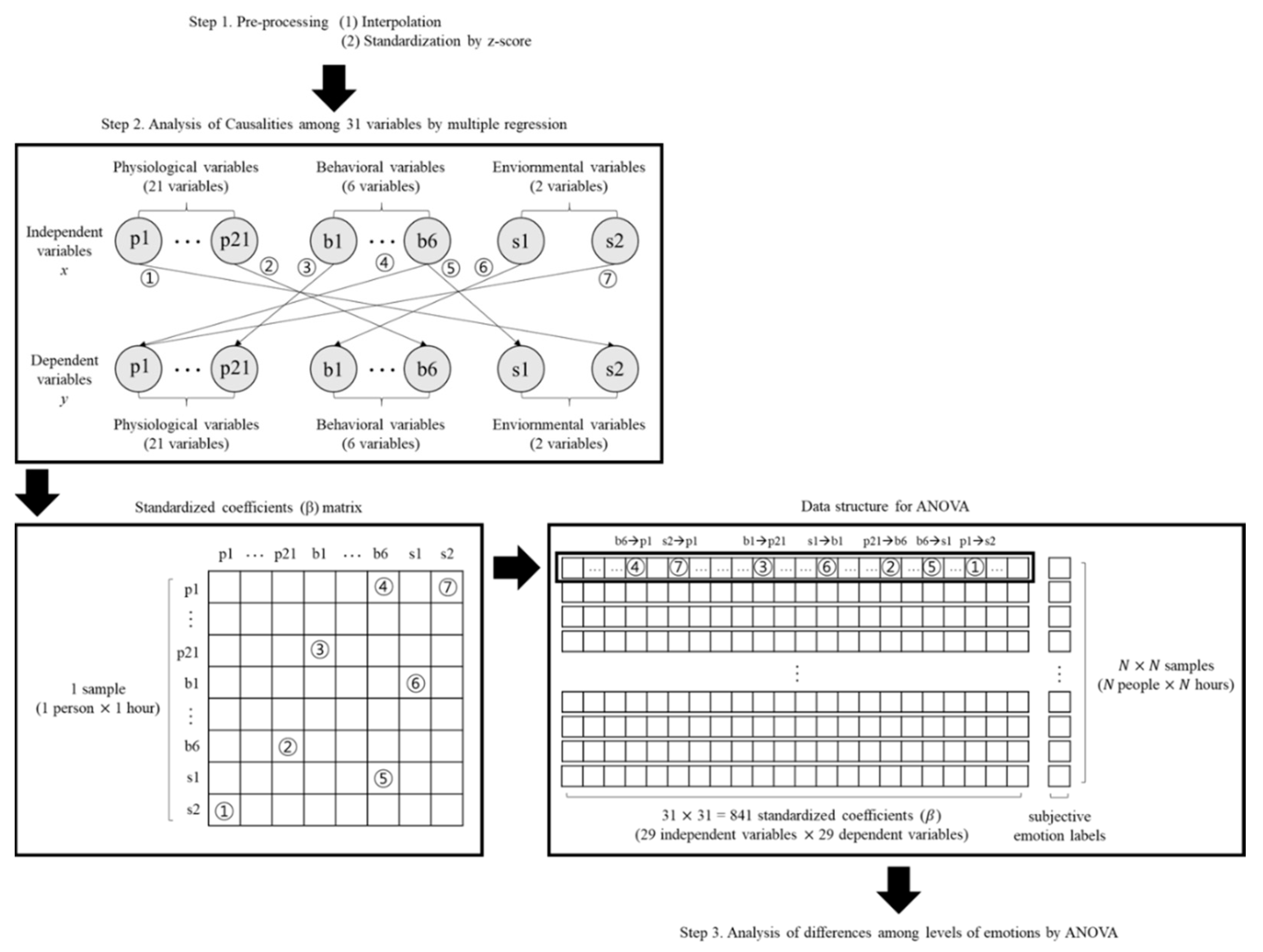
Figure 3.
Data structures of each analysis step. Standardized coefficients as results of multiple regression were formed as a matrix. Map the subjective emotion labels to the standardized coefficients matrix to form a data structure for ANOVA.
Figure 3.
Data structures of each analysis step. Standardized coefficients as results of multiple regression were formed as a matrix. Map the subjective emotion labels to the standardized coefficients matrix to form a data structure for ANOVA.
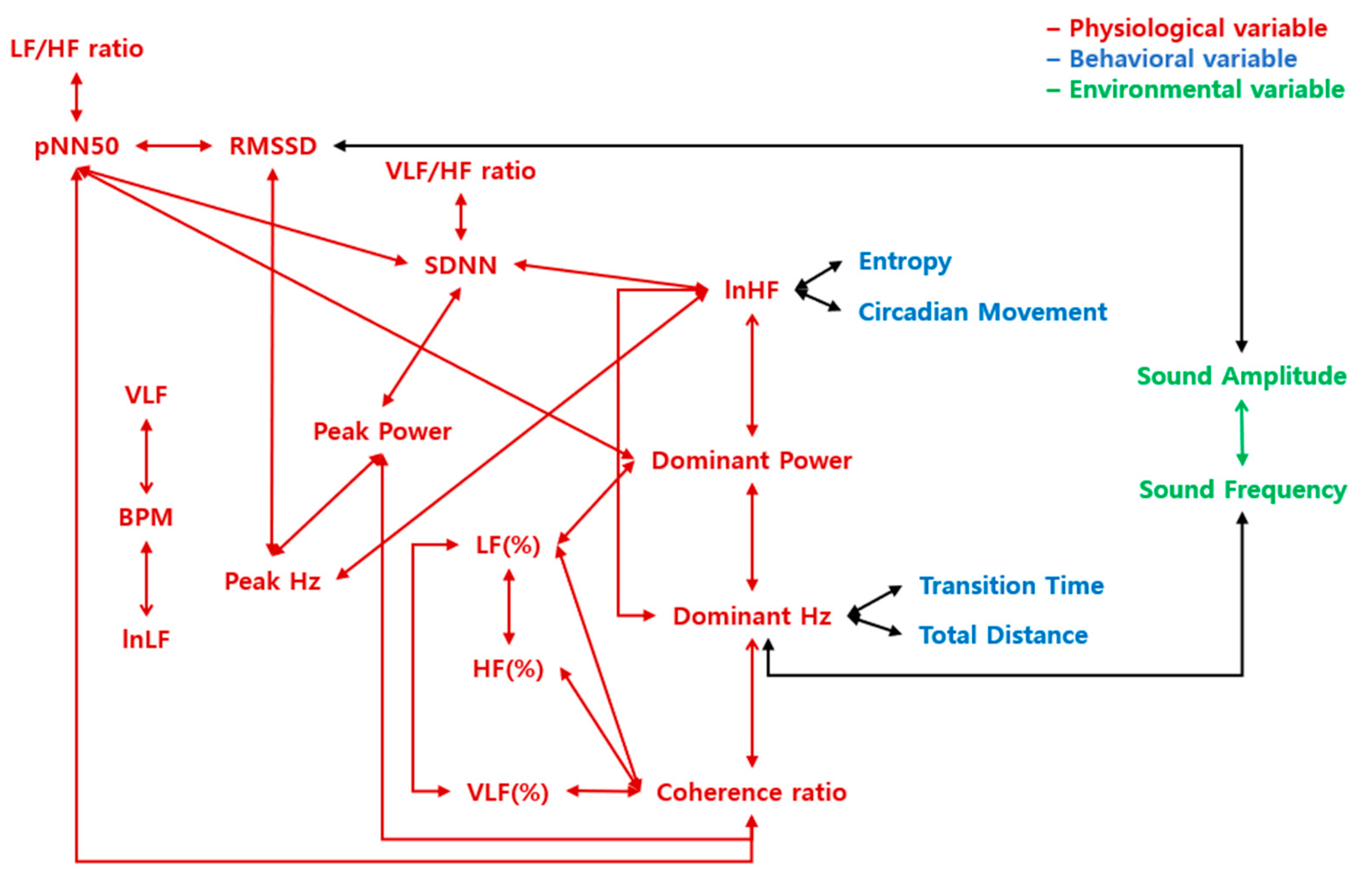
Figure 4.
A schematic representation of correlations that demonstrate the differences in arousal of emotions. The letters in red indicate physiological variables, blue indicate behavioral variables, and green indicate environmental variables. The arrows represent the correlation between the two variables. The red arrows represent the correlations within physiological variables, the green arrows represent the correlations within environmental variables, and the black arrows represent the correlations between the different construct variables.
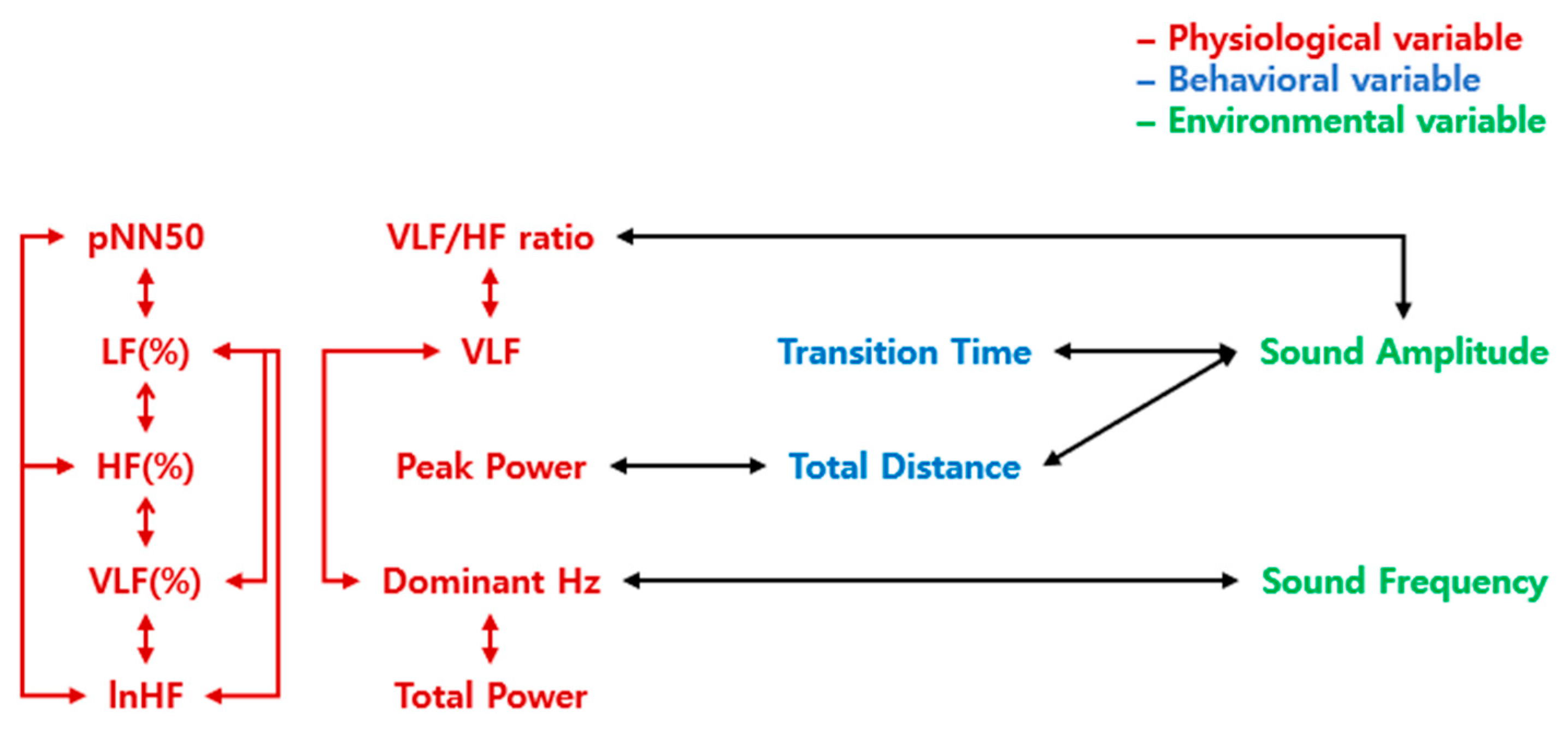
Figure 5.
A schematic representation of correlations that distinguish the differences in valence emotions. The letters in red indicate physiological variables, blue indicate behavioral variables, and green indicate environmental variables. The arrows represent the correlation between the two variables. The red arrows represent the correlations within physiological variables, the green arrows represent the correlations within environmental variables, and the black arrows represent the correlations between the different construct variables.
Table 1.
An example of the significant causalities analyzed by multiple regression among two weeks data for 79 participants. All assumptions of multiple regression were satisfied. There was no autocorrelation in the residuals (Durbin-Watson value = 2.264). Normality of residuals was satisfied (p-value of Kolmogorov-Smirnov test = 0.728). Homeogeneity of residuals was satisfied (p-value of Breusch-Pagan test = 0.499). Multiple regression was run to predict lnHF from location variance, circadian movement, transition time, total distance, total distance, pNN50, peak hz, and coherence ratio. Only those variables which were not affected by multicollinearity were entered in the multiple-regression (VIF < 10). A significant regression equation was found (F(25, 34) = 40.231, p < 0.000, Adj. = 0.943). Transition time was significant predictor of lnHF. Regression model degrees of freedom: 25, Residual degrees of freedom: 34, Autocorrelation Test - Durbin Watson: 2.264, Kolmogorov-Smirnov Test: Z = 0.089, p = 0.728, Breusch-Pagan Test: F = 0.994, p = 0.499.
| Dependent Variables | Tests | Statistics |
|---|
| lnHF | Multiple regression | Determining how well the model fits | Adj. R-square | 0.943 |
| F | 40.231 |
| Sig. | 0.000 |
| Statistical significance of the independent variables | Independent variables | Unstandardized coefficients (Beta) | p |
| (constant) | −10437988370.481 | 0.661 |
| Location Variance | 0.012 | 0.687 |
| Circadian Movement | 0.028 | 0.166 |
| Transition Time | −0.059 | 0.076 |
| Total Distance | 0.064 | 0.116 |
| pNN50 | 0.020 | 0.792 |
| Peak Hz | 0.050 | 0.115 |
| Coherence Ratio | 0.040 | 0.247 |
| Multicollinearity test | Independent variables | VIF |
| Location Variance | 2.759 |
| Circadian Movement | 3.673 |
| Transition Time | 7.764 |
| Total Distance | 8.050 |
| pNN50 | 8.528 |
| Peak Hz | 3.704 |
| Coherence Ratio | 4.322 |
Table 2.
Descriptive statistics of the standardized coefficients with significant differences between arousal levels.
Table 2.
Descriptive statistics of the standardized coefficients with significant differences between arousal levels.
| Variable | Descriptive Statistics of Standardized Coefficients |
|---|
| Independent | Dependent | Statistic | Arousal | Neutral | Relaxation |
|---|
| BPM | VLF | Mean | −5,745,442,617 | −17,308,431,507 | 8,428,219,435 |
| SD | 270,176,000,000 | 245,484,000,000 | 231,354,000,000 |
| pNN50 | Dominant Power | Mean | −0.423 | −0.613 | −0.659 |
| SD | 1.866 | 2.63 | 3.945 |
| RMSSD | pNN50 | Mean | 0.013 | 0.008 | 0.01 |
| SD | 0.05 | 0.041 | 0.046 |
| SDNN | pNN50 | Mean | 0.025 | 0.032 | 0.034 |
| SD | 0.071 | 0.099 | 0.089 |
| SDNN | lnHF | Mean | −0.055 | −0.05 | −0.141 |
| SD | 0.838 | 0.931 | 0.93 |
| SDNN | VLF/HF ratio | Mean | −0.001 | −0.003 | −0.007 |
| SD | 0.073 | 0.062 | 0.082 |
| SDNN | Peak Power | Mean | −0.045 | −0.089 | −0.056 |
| SD | 0.345 | 0.53 | 0.433 |
| LF(%) | VLF(%) | Mean | −0.001 | −0.003 | −0.006 |
| SD | 0.031 | 0.053 | 0.082 |
| LF(%) | HF(%) | Mean | −0.001 | −0.003 | −0.008 |
| SD | 0.04 | 0.068 | 0.098 |
| lnLF | BPM | Mean | 0.001 | 0 | −0.001 |
| SD | 0.022 | 0.017 | 0.022 |
| lnHF | Entropy | Mean | −1193.169 | −140,776.746 | 14,580.387 |
| SD | 37,241.047 | 3,206,125.223 | 642,719.545 |
| lnHF | Circadian Movement | Mean | 0 | 0.001 | 0 |
| SD | 0.006 | 0.016 | 0.004 |
| lnHF | Dominant Hz | Mean | −0.097 | −0.112 | −0.119 |
| SD | 0.236 | 0.249 | 0.254 |
| lnHF | Peak Hz | Mean | 0.032 | 0.04 | 0.041 |
| SD | 0.08 | 0.092 | 0.091 |
| LF/HF ratio | pNN50 | Mean | −0.004 | −0.006 | 0 |
| SD | 0.052 | 0.06 | 0.067 |
| Dominant Power | lnHF | Mean | −0.041 | 0.004 | 0.035 |
| SD | 0.902 | 0.853 | 0.872 |
| Dominant Hz | Dominant Power | Mean | −0.008 | −0.138 | −0.055 |
| SD | 0.791 | 2.046 | 1.176 |
| Dominant Hz | Coherence ratio | Mean | −0.042 | −0.06 | −0.064 |
| SD | 0.259 | 0.215 | 0.225 |
| Dominant Hz | Sound Frequency | Mean | −0.002 | −0.003 | 0.003 |
| SD | 0.077 | 0.051 | 0.044 |
| Peak Power | Coherence ratio | Mean | 0.156 | 0.127 | 0.111 |
| SD | 0.456 | 0.359 | 0.339 |
| Peak Hz | RMSSD | Mean | −0.075 | 0.2 | −0.013 |
| SD | 1.933 | 4.134 | 1.17 |
| Peak Hz | Peak Power | Mean | 0.043 | 0.119 | 0.216 |
| SD | 1.258 | 0.878 | 1.729 |
| Coherence ratio | pNN50 | Mean | 0.006 | −0.002 | 0.001 |
| SD | 0.077 | 0.08 | 0.076 |
| Coherence ratio | VLF(%) | Mean | −105,267,518.5 | −2,016,911,138 | −48,597,422.56 |
| SD | 15,299,232,245 | 17,846,539,923 | 20,110,510,824 |
| Coherence ratio | LF(%) | Mean | −132,068,389.2 | −2,021,703,780 | −84,532,472.78 |
| SD | 14,109,144,081 | 17,824,867,958 | 18,840,262,720 |
| Coherence ratio | HF(%) | Mean | −217,938,238.3 | −2,389,073,268 | −85,954,745.84 |
| SD | 16,032,965,209 | 21,954,646,140 | 22,568,564,779 |
| Coherence ratio | Dominant Hz | Mean | −0.065 | −0.074 | −0.093 |
| SD | 0.309 | 0.345 | 0.325 |
| Transition Time | Dominant Hz | Mean | −0.015 | −0.015 | 0.011 |
| SD | 0.259 | 0.175 | 0.194 |
| Total Distance | Dominant Hz | Mean | 0.009 | 0.019 | −0.003 |
| SD | 0.182 | 0.195 | 0.236 |
| Sound Amplitude | RMSSD | Mean | 0.005 | 0.376 | 0.02 |
| SD | 0.757 | 7.924 | 1.492 |
| Sound Amplitude | Sound Frequency | Mean | 0.062 | 0.078 | 0.094 |
| SD | 0.245 | 0.266 | 0.286 |
| Sound Frequency | Sound Amplitude | Mean | 0.075 | 0.086 | 0.109 |
| SD | 0.299 | 0.314 | 0.337 |
Table 3.
Descriptive statistics of the standardized coefficients with significant differences between valence levels.
Table 3.
Descriptive statistics of the standardized coefficients with significant differences between valence levels.
| Variable | Descriptive Statistics of Standardized Coefficients |
|---|
| Independent | Dependent | Statistic | Positive | Neutral | Negative |
|---|
| Total Distance | Peak Power | Mean | −0.033 | −0.128 | −0.01 |
| SD | 0.717 | 2.004 | 0.7510.751 |
| pNN50 | LF(%) | Mean | −118,639,038.5 | 1,079,730,567 | 1,891,445,746 |
| SD | 21,820,377,528 | 18,397,399,419 | 29,119,919,937 |
| pNN50 | HF(%) | Mean | −209,743,703.2 | 1,227,721,976 | 2,344,251,772 |
| SD | 25,563,848,513 | 21,374,411,771 | 35,526,468,774 |
| VLF(%) | LF(%) | Mean | −0.002 | −0.007 | −0.001 |
| SD | 0.041 | 0.081 | 0.036 |
| VLF(%) | HF(%) | Mean | −0.002 | −0.009 | −0.002 |
| SD | 0.052 | 0.104 | 0.046 |
| LF(%) | VLF(%) | Mean | −0.003 | −0.007 | −0.001 |
| SD | 0.055 | 0.088 | 0.029 |
| LF(%) | HF(%) | Mean | −0.003 | −0.009 | −0.001 |
| SD | 0.064 | 0.109 | 0.041 |
| HF(%) | VLF(%) | Mean | −0.002 | −0.006 | −0.001 |
| SD | 0.037 | 0.068 | 0.021 |
| HF(%) | LF(%) | Mean | −0.002 | −0.006 | −0.001 |
| SD | 0.036 | 0.066 | 0.022 |
| lnHF | VLF(%) | Mean | −6,230,158.347 | -808,663,867.5 | 139,285,674.2 |
| SD | 5,364,187,185 | 14,013,185,177 | 5,257,502,233 |
| lnHF | LF(%) | Mean | −5,812,633.013 | -910,997,723.4 | 128,324,064 |
| SD | 5,522,380,316 | 16,960,721,918 | 5,205,893,477 |
| lnHF | HF(%) | Mean | −19,292,545.01 | −1,142,833,043 | 160,581,520.7 |
| SD | 6,721,689,128 | 21,115,017,843 | 6,435,510,213 |
| VLF/HF ratio | VLF | Mean | −6,771,606,848 | 4806843674 | 5,214,155,475 |
| SD | 191,933,000,000 | 89,138,008,055 | 97,000,248,564 |
| VLF/HF ratio | Sound Amplitude | Mean | −0.001 | 0.007 | −0.002 |
| SD | 0.051 | 0.07 | 0.057 |
| Dominant Hz | VLF | Mean | 4,564,168,257 | 941,743,170 | −10,176,921,026 |
| SD | 93,659,975,658 | 111,036,000,000 | 224,181,000,000 |
| Dominant Hz | Total Power | Mean | −9,252,548,826 | 387775431.7 | 15,059,942,652 |
| SD | 190,801,000,000 | 222,377,000,000 | 381,999,000,000 |
| Sound Amplitude | Transition Time | Mean | 0.024 | −0.007 | 0.004 |
| SD | 0.327 | 0.395 | 0.227 |
| Sound Amplitude | Total Distance | Mean | −0.023 | 0.023 | 0.031 |
| SD | 0.49 | 0.481 | 0.789 |
| Sound Amplitude | VLF/HF ratio | Mean | −0.011 | 0.013 | 0.002 |
| SD | 0.285 | 0.141 | 0.304 |
| Sound Frequency | Dominant Hz | Mean | 0 | −0.01 | 0.008 |
| SD | 0.143 | 0.167 | 0.138 |
Table 4.
Results of one-way ANOVA show a significant difference between Arousal-Neutral-Relaxation among variables correlated with BPM analyzed by multiple regression. The difference between the two emotion levels was verified by independent t-test.
Table 4.
Results of one-way ANOVA show a significant difference between Arousal-Neutral-Relaxation among variables correlated with BPM analyzed by multiple regression. The difference between the two emotion levels was verified by independent t-test.
| Dependent variables | Tests | Statistics | lnLF |
|---|
| BPM | ANOVA | F | 3.173 |
| p | 0.042 |
| T-test | Arousal-Neutral | t | 1.487 |
| p | 0.137 |
| Neutral-Relaxation | t | 0.488 |
| p | 0.625 |
| Arousal-Relaxation | t | −2.358 |
| p | 0.018 |
Table 5.
Results of one-way ANOVA show a significant difference between Arousal-Neutral-Relaxation among variables correlated with RMSSD analyzed by multiple regression. The difference between the two emotion levels was verified by independent t-test.
Table 5.
Results of one-way ANOVA show a significant difference between Arousal-Neutral-Relaxation among variables correlated with RMSSD analyzed by multiple regression. The difference between the two emotion levels was verified by independent t-test.
| Dependent variables | Tests | Statistics | Peak Hz | Sound Amplitude |
|---|
| RMSSD | ANOVA | F | 4.067 | 3.466 |
| p | 0.017 | 0.031 |
| T-test | Arousal-Neutral | t | -2.346 | −2.023 |
| p | 0.019 | 0.043 |
| Neutral-Relaxation | t | 1.964 | 1.782 |
| p | 0.050 | 0.075 |
| Arousal-Relaxation | t | 1.143 | 0.401 |
| p | 0.253 | 0.688 |
Table 6.
Results of one-way ANOVA show a significant difference between Arousal-Neutral-Relaxation among variables correlated with pNN50 analyzed by multiple regression. The difference between the two emotion levels was verified by independent t-test.
Table 6.
Results of one-way ANOVA show a significant difference between Arousal-Neutral-Relaxation among variables correlated with pNN50 analyzed by multiple regression. The difference between the two emotion levels was verified by independent t-test.
| Dependent Variables | Tests | Statistics | SDNN | RMSSD | LF/HF ratio | Coherence Ratio |
|---|
| pNN50 | ANOVA | F | 5.367 | 4.233 | 3.496 | 3.946 |
| p | 0.005 | 0.015 | 0.030 | 0.019 |
| T-test | Arousal-Neutral | t | −2.200 | 2.625 | 0.969 | 2.502 |
| p | 0.028 | 0.009 | 0.332 | 0.012 |
| Neutral-Relaxation | t | −0.292 | −1.109 | −2.200 | −0.885 |
| p | 0.770 | 0.268 | 0.028 | 0.376 |
| Arousal-Relaxation | t | 3.257 | −2.004 | 1.994 | −2.092 |
| p | 0.001 | 0.045 | 0.046 | 0.036 |
Table 7.
Results of one-way ANOVA show a significant difference between Arousal-Neutral-Relaxation among variables correlated with VLF analyzed by multiple regression. The difference between the two emotion levels was verified by independent t-test.
Table 7.
Results of one-way ANOVA show a significant difference between Arousal-Neutral-Relaxation among variables correlated with VLF analyzed by multiple regression. The difference between the two emotion levels was verified by independent t-test.
| Dependent Variables | Tests | Statistics | BPM |
|---|
| VLF | ANOVA | F | 3.109 |
| p | 0.045 |
| T-test | Arousal-Neutral | t | 1.032 |
| p | 0.302 |
| Neutral-Relaxation | t | −2.518 |
| p | 0.012 |
| Arousal-Relaxation | t | 1.681 |
| p | 0.093 |
Table 8.
Results of one-way ANOVA show a significant difference between Arousal-Neutral-Relaxation among variables correlated with VLF(%) analyzed by multiple regression. The difference between the two emotion levels was verified by independent t-test.
Table 8.
Results of one-way ANOVA show a significant difference between Arousal-Neutral-Relaxation among variables correlated with VLF(%) analyzed by multiple regression. The difference between the two emotion levels was verified by independent t-test.
| Dependent Variables | Tests | Statistics | LF(%) | Coherence Ratio |
|---|
| VLF(%) | ANOVA | F | 3.597 | 3.813 |
| p | 0.027 | 0.022 |
| T-test | Arousal-Neutral | t | 1.022 | 2.793 |
| p | 0.307 | 0.005 |
| Neutral-Relaxation | t | 1.117 | −2.338 |
| p | 0.264 | 0.019 |
| Arousal-Relaxation | t | −2.604 | 0.096 |
| p | 0.009 | 0.924 |
Table 9.
Results of one-way ANOVA show a significant difference between Arousal-Neutral-Relaxation among variables correlated with LF(%) analyzed by multiple regression. The difference between the two emotion levels was verified by independent t-test.
Table 9.
Results of one-way ANOVA show a significant difference between Arousal-Neutral-Relaxation among variables correlated with LF(%) analyzed by multiple regression. The difference between the two emotion levels was verified by independent t-test.
| Dependent Variables | Tests | Statistics | Coherence Ratio |
|---|
| LF(%) | ANOVA | F | 4.166 |
| p | 0.016 |
| T-test | Arousal-Neutral | t | 2.905 |
| p | 0.004 |
| Neutral-Relaxation | t | −2.413 |
| p | 0.016 |
| Arousal-Relaxation | t | 0.086 |
| p | 0.931 |
Table 10.
Results of one-way ANOVA show a significant difference between Arousal-Neutral-Relaxation among variables correlated with HF(%) analyzed by multiple regression. The difference between the two emotion levels was verified by independent t-test.
Table 10.
Results of one-way ANOVA show a significant difference between Arousal-Neutral-Relaxation among variables correlated with HF(%) analyzed by multiple regression. The difference between the two emotion levels was verified by independent t-test.
| Dependent Variables | Tests | Statistics | LF(%) | Coherence Ratio |
|---|
| HF(%) | ANOVA | F | 3.375 | 4.056 |
| p | 0.034 | 0.017 |
| T-test | Arousal-Neutral | t | 1.023 | 2.841 |
| p | 0.306 | 0.005 |
| Neutral-Relaxation | t | 1.050 | −2.376 |
| p | 0.294 | 0.018 |
| Arousal-Relaxation | t | −2.550 | 0.204 |
| p | 0.011 | 0.838 |
Table 11.
Results of one-way ANOVA show a significant difference between Arousal-Neutral-Relaxation among variables correlated with lnHF analyzed by multiple regression. The difference between the two emotion levels was verified by independent t-test.
Table 11.
Results of one-way ANOVA show a significant difference between Arousal-Neutral-Relaxation among variables correlated with lnHF analyzed by multiple regression. The difference between the two emotion levels was verified by independent t-test.
| Dependent Variables | Tests | Statistics | SDNN | Dominant Power |
|---|
| lnHF | ANOVA | F | 4.967 | 3.343 |
| p | 0.007 | 0.035 |
| T-test | Arousal-Neutral | t | −0.150 | −1.178 |
| p | 0.881 | 0.239 |
| Neutral-Relaxation | t | 2.256 | −0.832 |
| p | 0.024 | 0.406 |
| Arousal-Relaxation | t | −2.901 | 2.556 |
| p | 0.004 | 0.011 |
Table 12.
Results of one-way ANOVA show a significant difference between Arousal-Neutral-Relaxation among variables correlated with VLF/HF ratio analyzed by multiple regression. The difference between the two emotion levels was verified by independent t-test.
Table 12.
Results of one-way ANOVA show a significant difference between Arousal-Neutral-Relaxation among variables correlated with VLF/HF ratio analyzed by multiple regression. The difference between the two emotion levels was verified by independent t-test.
| Dependent Variables | Tests | Statistics | SDNN |
|---|
| VLF/HF ratio | ANOVA | F | 3.417 |
| p | 0.033 |
| T-test | Arousal-Neutral | t | 0.474 |
| p | 0.636 |
| Neutral-Relaxation | t | 1.509 |
| p | 0.132 |
| Arousal-Relaxation | t | −2.475 |
| p | 0.013 |
Table 13.
Results of one-way ANOVA show a significant difference between Arousal-Neutral-Relaxation among variables correlated with Peak Power analyzed by multiple regression. The difference between the two emotion levels was verified by independent t-test.
Table 13.
Results of one-way ANOVA show a significant difference between Arousal-Neutral-Relaxation among variables correlated with Peak Power analyzed by multiple regression. The difference between the two emotion levels was verified by independent t-test.
| Dependent Variables | Tests | Statistics | SDNN | Peak Hz |
|---|
| Peak Power | ANOVA | F | 3.013 | 6.761 |
| p | 0.049 | 0.001 |
| T-test | Arousal-Neutral | t | 2.513 | −1.537 |
| p | 0.012 | 0.124 |
| Neutral-Relaxation | t | −1.600 | −1.476 |
| p | 0.110 | 0.140 |
| Arousal-Relaxation | t | −0.873 | 3.456 |
| p | 0.383 | 0.001 |
Table 14.
Results of one-way ANOVA show a significant difference between Arousal-Neutral-Relaxation among variables correlated with Peak Hz analyzed by multiple regression. The difference between the two emotion levels was verified by independent t-test.
Table 14.
Results of one-way ANOVA show a significant difference between Arousal-Neutral-Relaxation among variables correlated with Peak Hz analyzed by multiple regression. The difference between the two emotion levels was verified by independent t-test.
| Dependent Variables | Tests | Statistics | lnHF |
|---|
| Peak Hz | ANOVA | F | 5.202 |
| p | 0.006 |
| T-test | Arousal-Neutral | t | −2.246 |
| p | 0.025 |
| Neutral-Relaxation | t | −0.179 |
| p | 0.858 |
| Arousal-Relaxation | t | 3.058 |
| p | 0.002 |
Table 15.
Results of one-way ANOVA show a significant difference between Arousal-Neutral-Relaxation among variables correlated with Coherence ratio analyzed by multiple regression. The difference between the two emotion levels was verified by independent t-test.
Table 15.
Results of one-way ANOVA show a significant difference between Arousal-Neutral-Relaxation among variables correlated with Coherence ratio analyzed by multiple regression. The difference between the two emotion levels was verified by independent t-test.
| Dependent Variables | Tests | Statistics | Dominant Hz | Peak Power |
|---|
| Coherence ratio | ANOVA | F | 4.194 | 5.807 |
| p | 0.015 | 0.003 |
| T-test | Arousal-Neutral | t | 1.690 | 1.553 |
| p | 0.091 | 0.120 |
| Neutral-Relaxation | t | 0.466 | 1.090 |
| p | 0.641 | 0.276 |
| Arousal-Relaxation | t | −2.737 | −3.311 |
| p | 0.006 | 0.001 |
Table 16.
Results of one-way ANOVA show a significant difference between Arousal-Neutral-Relaxation among variables correlated with Dominant Power analyzed by multiple regression. The difference between the two emotion levels was verified by independent t-test.
Table 16.
Results of one-way ANOVA show a significant difference between Arousal-Neutral-Relaxation among variables correlated with Dominant Power analyzed by multiple regression. The difference between the two emotion levels was verified by independent t-test.
| Dependent Variables | Tests | Statistics | pNN50 | Dominant Hz |
|---|
| Dominant Power | ANOVA | F | 3.095 | 3.013 |
| p | 0.045 | 0.049 |
| T-test | Arousal-Neutral | t | 2.117 | 2.365 |
| p | 0.034 | 0.018 |
| Neutral-Relaxation | t | 0.296 | −1.278 |
| p | 0.767 | 0.201 |
| Arousal-Relaxation | t | −2.342 | −1.400 |
| p | 0.019 | 0.162 |
Table 17.
Results of one-way ANOVA show a significant difference between Arousal-Neutral-Relaxation among variables correlated with Dominant Hz analyzed by multiple regression. The difference between the two emotion levels was verified by independent t-test.
Table 17.
Results of one-way ANOVA show a significant difference between Arousal-Neutral-Relaxation among variables correlated with Dominant Hz analyzed by multiple regression. The difference between the two emotion levels was verified by independent t-test.
| Dependent Variables | Tests | Statistics | Transition Time | Total Distance | lnHF | Coherence Ratio |
|---|
| Dominant Hz | ANOVA | F | 6.946 | 3.524 | 3.559 | 3.252 |
| p | 0.001 | 0.030 | 0.029 | 0.039 |
| T-test | Arousal-Neutral | t | 0.014 | 0.014 | 1.407 | 0.626 |
| p | 0.989 | 0.989 | 0.159 | 0.531 |
| Neutral-Relaxation | t | −3.155 | −3.155 | 0.657 | 1.297 |
| p | 0.002 | 0.002 | 0.511 | 0.195 |
| Arousal-Relaxation | t | 3.326 | 3.326 | −2.642 | −2.570 |
| p | 0.001 | 0.001 | 0.008 | 0.010 |
Table 18.
Results of one-way ANOVA show a significant difference between Arousal-Neutral-Relaxation among variables correlated with Entropy analyzed by multiple regression. The difference between the two emotion levels was verified by independent t-test.
Table 18.
Results of one-way ANOVA show a significant difference between Arousal-Neutral-Relaxation among variables correlated with Entropy analyzed by multiple regression. The difference between the two emotion levels was verified by independent t-test.
| Dependent Variables | Tests | Statistics | lnHF |
|---|
| Entropy | ANOVA | F | 3.538 |
| p | 0.029 |
| T-test | Arousal-Neutral | t | 1.900 |
| p | 0.058 |
| Neutral-Relaxation | t | −1.914 |
| p | 0.056 |
| Arousal-Relaxation | t | 1.069 |
| p | 0.285 |
Table 19.
Results of one-way ANOVA show a significant difference between Arousal-Neutral-Relaxation among variables correlated with Circadian Movement analyzed by multiple regression. The difference between the two emotion levels was verified by independent t-test.
Table 19.
Results of one-way ANOVA show a significant difference between Arousal-Neutral-Relaxation among variables correlated with Circadian Movement analyzed by multiple regression. The difference between the two emotion levels was verified by independent t-test.
| Dependent Variables | Tests | Statistics | lnHF |
|---|
| Circadian Movement | ANOVA | F | 3.648 |
| p | 0.026 |
| T-test | Arousal-Neutral | t | −2.202 |
| p | 0.028 |
| Neutral-Relaxation | t | 1.621 |
| p | 0.105 |
| Arousal-Relaxation | t | 1.614 |
| p | 0.107 |
Table 20.
Results of one-way ANOVA show a significant difference between Arousal-Neutral-Relaxation among variables correlated with Sound Amplitude analyzed by multiple regression. The difference between the two emotion levels was verified by independent t-test.
Table 20.
Results of one-way ANOVA show a significant difference between Arousal-Neutral-Relaxation among variables correlated with Sound Amplitude analyzed by multiple regression. The difference between the two emotion levels was verified by independent t-test.
| Dependent Variables | Tests | Statistics | Sound Frequency |
|---|
| Sound Amplitude | ANOVA | F | 5.174 |
| p | 0.006 |
| T-test | Arousal-Neutral | t | −0.878 |
| p | 0.380 |
| Neutral-Relaxation | t | −1.571 |
| p | 0.116 |
| Arousal-Relaxation | t | 3.191 |
| p | 0.001 |
Table 21.
Results of one-way ANOVA show a significant difference between Arousal-Neutral-Relaxation among variables correlated with Sound Frequency analyzed by multiple regression. The difference between the two emotion levels was verified by independent t-test.
Table 21.
Results of one-way ANOVA show a significant difference between Arousal-Neutral-Relaxation among variables correlated with Sound Frequency analyzed by multiple regression. The difference between the two emotion levels was verified by independent t-test.
| Dependent variables | Tests | Statistics | Dominant Hz | Sound Amplitude |
|---|
| Sound Frequency | ANOVA | F | 3.314 | 6.380 |
| p | 0.036 | 0.002 |
| T-test | Arousal-Neutral | t | 0.359 | −1.420 |
| p | 0.720 | 0.156 |
| Neutral-Relaxation | t | −2.788 | −1.355 |
| p | 0.005 | 0.175 |
| Arousal-Relaxation | t | 2.141 | 3.574 |
| p | 0.032 | 0.000 |
Table 22.
Results of ANOVA show a significant difference between Positive-Neutral-Negative among variables correlated with VLF analyzed by multiple regression. The difference between the two emotion levels was verified by independent t-test.
Table 22.
Results of ANOVA show a significant difference between Positive-Neutral-Negative among variables correlated with VLF analyzed by multiple regression. The difference between the two emotion levels was verified by independent t-test.
| Dependent Variables | Tests | Statistics | VLF/HF Ratio | Dominant Hz |
|---|
| VLF | ANOVA | F | 3.238 | 4.067 |
| p | 0.039 | 0.017 |
| T-test | Positive-Neutral | t | −1.811 | 0.959 |
| p | 0.07 | 0.338 |
| Neutral-Negative | t | −0.099 | 1.409 |
| p | 0.921 | 0.159 |
| Positive-Negative | t | 1.953 | −2.698 |
| p | 0.051 | 0.007 |
Table 23.
Results of one-way ANOVA show a significant difference between Positive-Neutral-Negative among variables correlated with VLF(%) analyzed by multiple regression. The difference between the two emotion levels was verified by independent t-test.
Table 23.
Results of one-way ANOVA show a significant difference between Positive-Neutral-Negative among variables correlated with VLF(%) analyzed by multiple regression. The difference between the two emotion levels was verified by independent t-test.
| Dependent Variables | Tests | Statistics | LF(%) | HF(%) | lnHF |
|---|
| VLF(%) | ANOVA | F | 3.359 | 4.107 | 4.281 |
| p | 0.035 | 0.017 | 0.014 |
| T-test | Positive-Neutral | t | 1.82 | 2.166 | 2.37 |
| p | 0.069 | 0.03 | 0.018 |
| Neutral-Negative | t | −2.329 | −2.366 | −2.083 |
| p | 0.02 | 0.018 | 0.037 |
| Positive-Negative | t | 1.094 | 0.913 | 0.744 |
| p | 0.274 | 0.361 | 0.457 |
Table 24.
Results of one-way ANOVA show a significant difference between Positive-Neutral-Negative among variables correlated with LF(%) analyzed by multiple regression. The difference between the two emotion levels was verified by independent t-test.
Table 24.
Results of one-way ANOVA show a significant difference between Positive-Neutral-Negative among variables correlated with LF(%) analyzed by multiple regression. The difference between the two emotion levels was verified by independent t-test.
| Dependent Variables | Tests | Statistics | pNN50 | VLF(%) | HF(%) | lnHF |
|---|
| LF(%) | ANOVA | F | 3.001 | 3.872 | 3.952 | 4.002 |
| p | 0.05 | 0.021 | 0.019 | 0.018 |
| T-test | Positive-Neutral | t | −1.509 | 2.394 | 2.145 | 2.291 |
| p | 0.131 | 0.017 | 0.032 | 0.022 |
| Neutral-Negative | t | −0.75 | −1.997 | −2.315 | −1.931 |
| p | 0.453 | 0.046 | 0.021 | 0.054 |
| Positive-Negative | t | 2.243 | 0.185 | 0.861 | 0.674 |
| p | 0.025 | 0.853 | 0.389 | 0.5 |
Table 25.
Results of one-way ANOVA show a significant difference between Positive-Neutral-Negative among variables correlated with HF(%) analyzed by multiple regression. The difference between the two emotion levels was verified by independent t-test.
Table 25.
Results of one-way ANOVA show a significant difference between Positive-Neutral-Negative among variables correlated with HF(%) analyzed by multiple regression. The difference between the two emotion levels was verified by independent t-test.
| Dependent Variables | Tests | Statistics | pNN50 | VLF(%) | LF(%) | lnHF |
|---|
| HF(%) | ANOVA | F | 3.367 | 3.938 | 3.438 | 4.057 |
| p | 0.035 | 0.02 | 0.032 | 0.017 |
| T-test | Positive-Neutral | t | −1.548 | 2.415 | 1.941 | 2.294 |
| p | 0.122 | 0.016 | 0.052 | 0.022 |
| Neutral-Negative | t | −0.857 | −2.014 | −2.244 | −1.946 |
| p | 0.392 | 0.044 | 0.025 | 0.052 |
| Positive-Negative | t | 2.387 | 0.204 | 0.953 | 0.739 |
| p | 0.017 | 0.839 | 0.341 | 0.46 |
Table 26.
Results of one-way ANOVA show a significant difference between Positive-Neutral-Negative among variables correlated with VLF/HF ratio analyzed by multiple regression. The difference between the two emotion levels was verified by independent t-test.
Table 26.
Results of one-way ANOVA show a significant difference between Positive-Neutral-Negative among variables correlated with VLF/HF ratio analyzed by multiple regression. The difference between the two emotion levels was verified by independent t-test.
| Dependent Variables | Tests | Statistics | Sound Amplitude |
|---|
| VLF/HF ratio | ANOVA | F | 3.149 |
| p | 0.043 |
| T-test | Positive-Neutral | t | −2.552 |
| p | 0.011 |
| Neutral-Negative | t | 1.008 |
| p | 0.313 |
| Positive-Negative | t | 1.28 |
| p | 0.201 |
Table 27.
Results of one-way ANOVA show a significant difference between Positive-Neutral-Negative among variables correlated with Peak Power analyzed by multiple regression. The difference between the two emotion levels was verified by independent t-test.
Table 27.
Results of one-way ANOVA show a significant difference between Positive-Neutral-Negative among variables correlated with Peak Power analyzed by multiple regression. The difference between the two emotion levels was verified by independent t-test.
| Dependent Variables | Tests | Statistics | Total Distance |
|---|
| Peak Power | ANOVA | F | 3.186 |
| p | 0.041 |
| T-test | Positive-Neutral | t | 1.991 |
| p | 0.047 |
| Neutral-Negative | t | −1.81 |
| p | 0.07 |
| Positive-Negative | t | 0.858 |
| p | 0.391 |
Table 28.
Results of one-way ANOVA show a significant difference between Positive-Neutral-Negative among variables correlated with Dominant Hz analyzed by multiple regression. The difference between the two emotion levels was verified by independent t-test.
Table 28.
Results of one-way ANOVA show a significant difference between Positive-Neutral-Negative among variables correlated with Dominant Hz analyzed by multiple regression. The difference between the two emotion levels was verified by independent t-test.
| Dependent Variables | Tests | Statistics | Sound Frequency |
|---|
| Dominant Hz | ANOVA | F | 3.826 |
| p | 0.022 |
| T-test | Positive-Neutral | t | 1.784 |
| p | 0.075 |
| Neutral-Negative | t | −2.671 |
| p | 0.008 |
| Positive-Negative | t | 1.473 |
| p | 0.141 |
Table 29.
Results of one-way ANOVA show a significant difference between Positive-Neutral-Negative among variables correlated with Total Power analyzed by multiple regression. The difference between the two emotion levels was verified by independent t-test.
Table 29.
Results of one-way ANOVA show a significant difference between Positive-Neutral-Negative among variables correlated with Total Power analyzed by multiple regression. The difference between the two emotion levels was verified by independent t-test.
| Dependent Variables | Tests | Statistics | Dominant Hz |
|---|
| Total Power | ANOVA | F | 3.305 |
| p | 0.037 |
| T-test | Positive-Neutral | t | −1.26 |
| p | 0.208 |
| Neutral-Negative | t | −1.055 |
| p | 0.291 |
| Positive-Negative | t | 2.473 |
| p | 0.013 |
Table 30.
Results of one-way ANOVA show a significant difference between Positive-Neutral-Negative among variables correlated with Total Distance analyzed by multiple regression. The difference between the two emotion levels was verified by independent t-test.
Table 30.
Results of one-way ANOVA show a significant difference between Positive-Neutral-Negative among variables correlated with Total Distance analyzed by multiple regression. The difference between the two emotion levels was verified by independent t-test.
| Dependent Variables | Tests | Statistics | Sound Amplitude |
|---|
| Total Distance | ANOVA | F | 4.284 |
| p | 0.014 |
| T-test | Positive-Neutral | t | −2.509 |
| p | 0.012 |
| Neutral-Negative | t | −0.28 |
| p | 0.779 |
| Positive-Negative | t | 2.473 |
| p | 0.013 |
Table 31.
Results of one-way ANOVA show a significant difference between Positive-Neutral-Negative among variables correlated with Transition Time analyzed by multiple regression. The difference between the two emotion levels was verified by independent t-test.
Table 31.
Results of one-way ANOVA show a significant difference between Positive-Neutral-Negative among variables correlated with Transition Time analyzed by multiple regression. The difference between the two emotion levels was verified by independent t-test.
| Dependent Variables | Tests | Statistics | Sound Amplitude |
|---|
| Transition Time | ANOVA | F | 3.66 |
| p | 0.026 |
| T-test | Positive-Neutral | t | 2.333 |
| p | 0.02 |
| Neutral-Negative | t | −0.769 |
| p | 0.442 |
| Positive-Negative | t | −1.852 |
| p | 0.064 |
Table 32.
Results of one-way ANOVA show a significant difference between Positive-Neutral-Negative among variables correlated with Sound Amplitude analyzed by multiple regression. The difference between the two emotion levels was verified by independent t-test.
Table 32.
Results of one-way ANOVA show a significant difference between Positive-Neutral-Negative among variables correlated with Sound Amplitude analyzed by multiple regression. The difference between the two emotion levels was verified by independent t-test.
| Dependent Variables | Tests | Statistics | VLF/HF Ratio |
|---|
| Sound Amplitude | ANOVA | F | 6.852 |
| p | 0.001 |
| T-test | Positive-Neutral | t | −3.389 |
| p | 0.001 |
| Neutral-Negative | t | 2.918 |
| p | 0.004 |
| Positive-Negative | t | −0.374 |
| p | 0.708 |


