Automatic Identification and Intuitive Map Representation of the Epiretinal Membrane Presence in 3D OCT Volumes

 ,
,  ,
,  , and
, and 
Abstract
1. Introduction
2. Materials and Methods
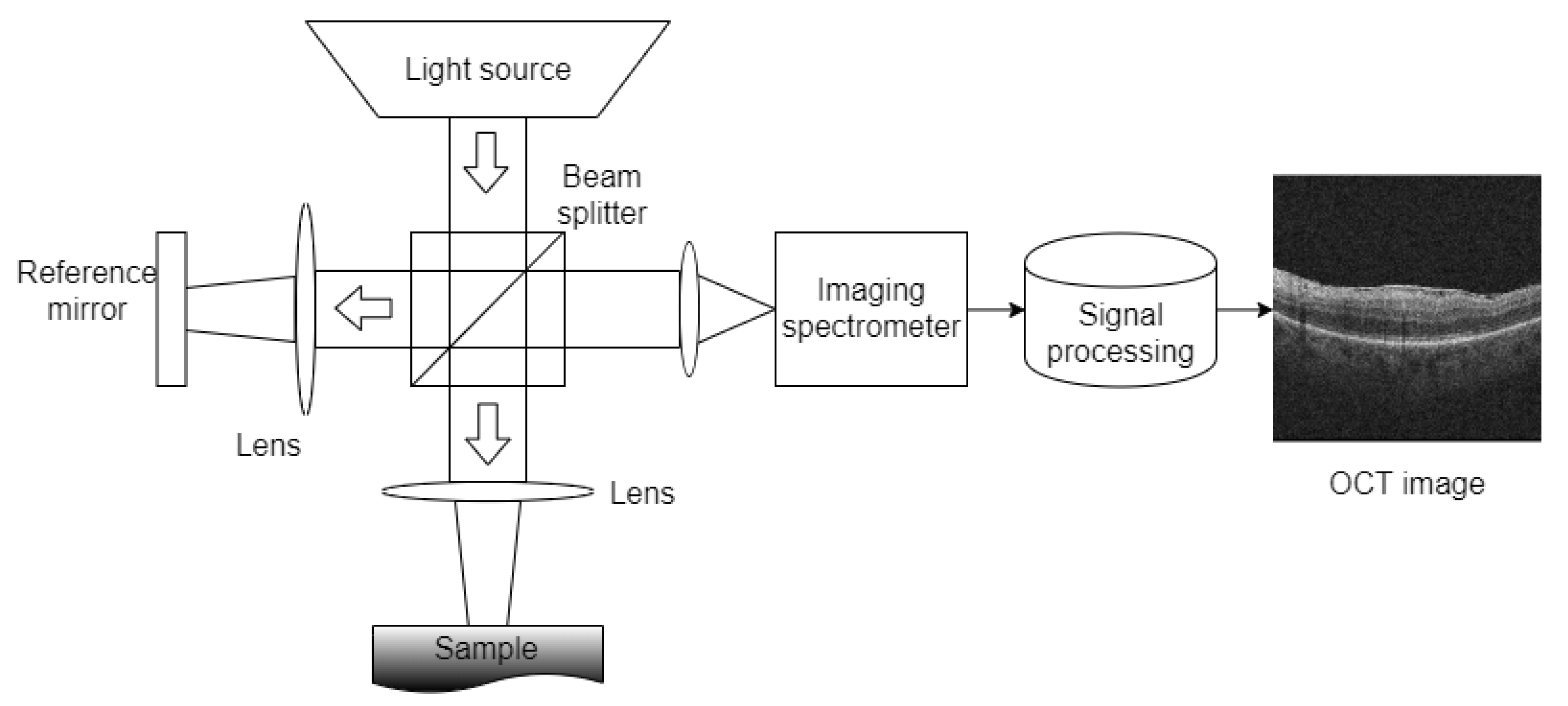
2.1. Acquisition
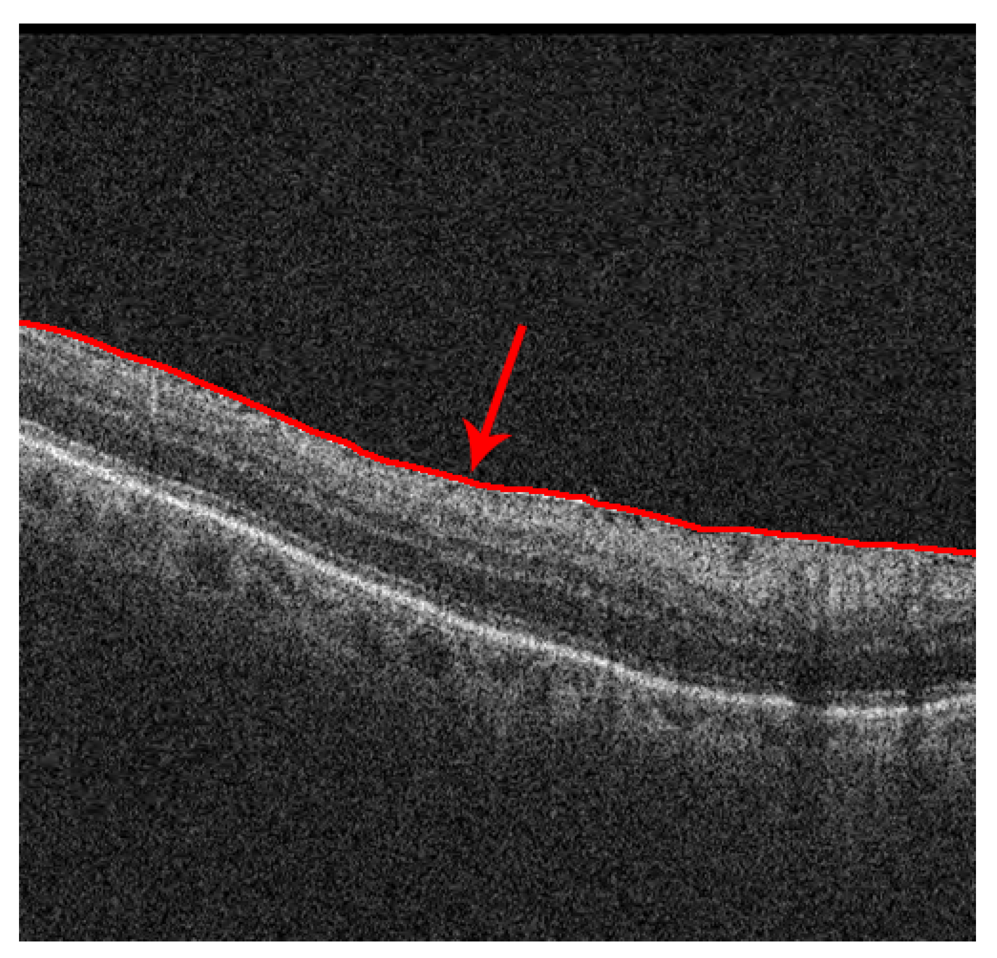
2.2. Identification of the Region of Interest
2.3. Feature Definition and Extraction
2.4. Feature Selection and Model Training
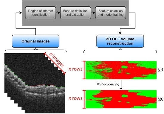
2.5. 3D OCT Volume Reconstruction and Map Generation
2.6. Post-Processing Map Refinement
3. Results
3.1. Feature Selection and Model Performance
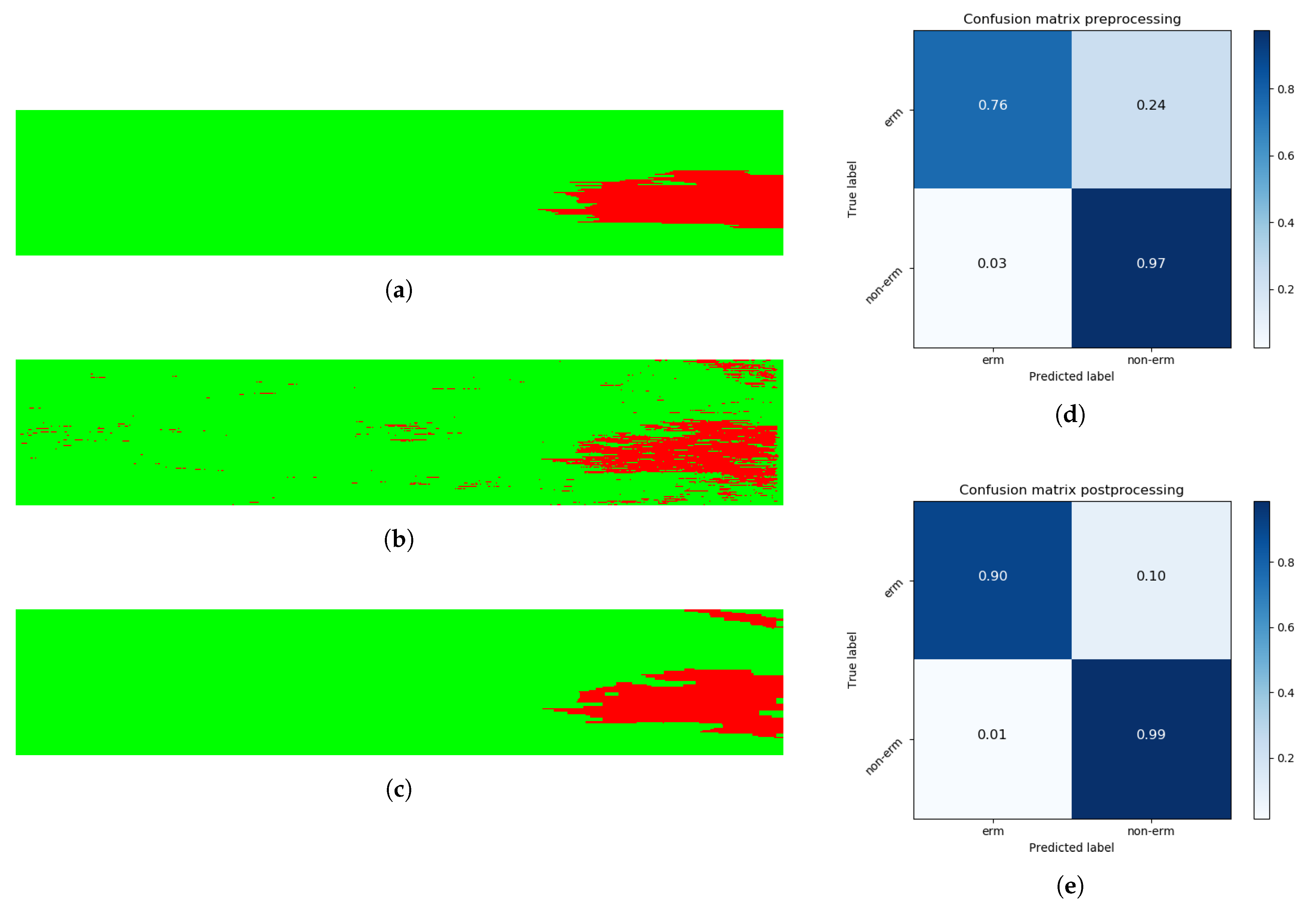
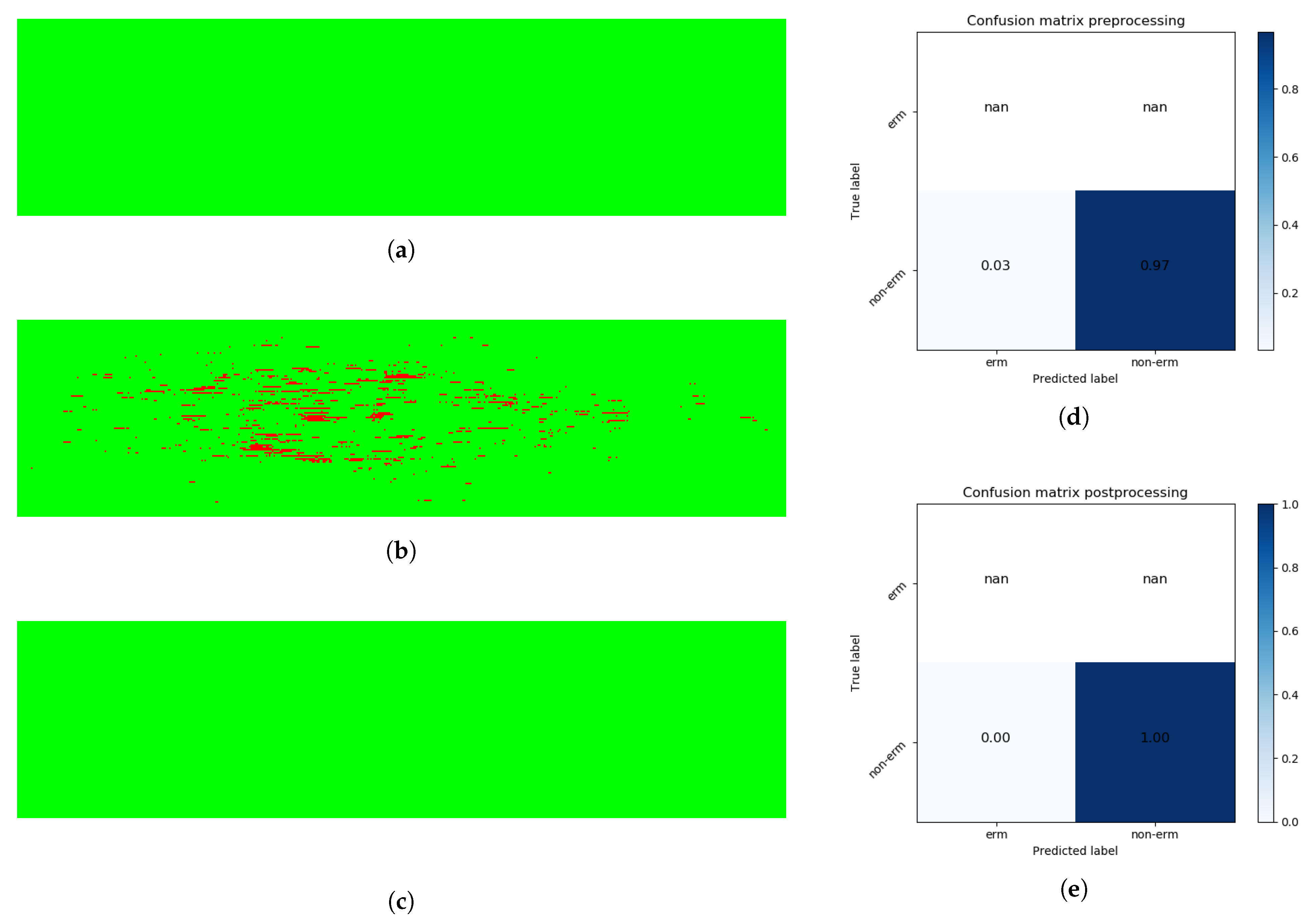
3.2. Pathological Map Generation and Final Post-Processing Stage
4. Discussion
5. Conclusions
Author Contributions
Funding
Conflicts of Interest
References
- Fernández, D.C.; Salinas, H.M.; Puliafito, C.A. Automated Detection of Retinal Layer Structures on Optical Coherence Tomography Images. Opt. Express 2005, 13, 10200–10216. [Google Scholar] [CrossRef] [PubMed]
- Kugelman, J.; Alonso-Caneiro, D.; Read, S.A.; Vincent, S.J.; Collins, M.J. Automatic Segmentation of OCT Retinal Boundaries Using Recurrent Neural Networks and Graph Search. Biomed. Opt. Express 2018, 9, 5759–5777. [Google Scholar] [CrossRef] [PubMed]
- Savastano, M.C.; Lumbroso, B.; Rispoli, M. In Vivo Characterization of Retinal Vascularization Morphology Using Optical Coherence Tomography Angiography. RETINA 2015, 35, 2196. [Google Scholar] [CrossRef] [PubMed]
- Margolis, R.; Spaide, R.F. A Pilot Study of Enhanced Depth Imaging Optical Coherence Tomography of the Choroid in Normal Eyes. Am. J. Ophthalmol. 2009, 147, 811–815. [Google Scholar] [CrossRef]
- Kelty, P.J.; Payne, J.F.; Trivedi, R.H.; Kelty, J.; Bowie, E.M.; Burger, B.M. Macular Thickness Assessment in Healthy Eyes Based on Ethnicity Using Stratus OCT Optical Coherence Tomography. Investig. Ophthalmol. Vis. Sci. 2008, 49, 2668–2672. [Google Scholar] [CrossRef]
- Savini, G.; Zanini, M.; Carelli, V.; Sadun, A.A.; Ross-Cisneros, F.N.; Barboni, P. Correlation between Retinal Nerve Fibre Layer Thickness and Optic Nerve Head Size: An Optical Coherence Tomography Study. Br. J. Ophthalmol. 2005, 89, 489–492. [Google Scholar] [CrossRef]
- Manjunath, V.; Taha, M.; Fujimoto, J.G.; Duker, J.S. Choroidal Thickness in Normal Eyes Measured Using Cirrus HD Optical Coherence Tomography. Am. J. Ophthalmol. 2010, 150, 325–329. [Google Scholar] [CrossRef]
- Ly, A.; Nivison-Smith, L.; Assaad, N.; Kalloniatis, M. Infrared Reflectance Imaging in Age-Related Macular Degeneration. Ophthalmic Physiol. Opt. 2016, 36, 303–316. [Google Scholar] [CrossRef]
- Watanabe, A.; Arimoto, S.; Nishi, O. Correlation between Metamorphopsia and Epiretinal Membrane Optical Coherence Tomography Findings. Ophthalmology 2009, 116, 1788–1793. [Google Scholar] [CrossRef]
- Wong, J.G.; Sachdev, N.; Beaumont, P.E.; Chang, A.A. Visual Outcomes Following Vitrectomy and Peeling of Epiretinal Membrane. Clin. Exp. Ophthalmol. 2005, 33, 373–378. [Google Scholar] [CrossRef]
- Flaxel, C.J.; Edwards, A.R.; Aiello, L.P.; Arrigg, P.G.; Beck, R.W.; Bressler, N.M.; Bressler, S.B.; Ferris, F.L.; Gupta, S.K.; Haller, J.A.; et al. Factors Associated with Visual Acuity Outcomes after Vitrectomy for Diabetic Macular Edema: Diabetic Retinopathy Clinical Research Network. Retin. (Phila. Pa.) 2010, 30, 1488–1495. [Google Scholar] [CrossRef] [PubMed]
- Ding, J.; Wong, T.Y. Current Epidemiology of Diabetic Retinopathy and Diabetic Macular Edema. Curr. Diabetes Rep. 2012, 12, 346–354. [Google Scholar] [CrossRef] [PubMed]
- Matthews, D.R.; Stratton, I.M.; Aldington, S.J.; Holman, R.R.; Kohner, E.M. Risks of Progression of Retinopathy and Vision Loss Related to Tight Blood Pressure Control in Type 2 Diabetes Mellitus: UKPDS 69. Arch. Ophthalmol. (Chic. Ill. 1960) 2004, 122, 1631–1640. [Google Scholar] [CrossRef]
- Sjølie, A.K.; Stephenson, J.; Aldington, S.; Kohner, E.; Janka, H.; Stevens, L.; Fuller, J.; Karamanos, B.; Tountas, C.; Kofinis, A.; et al. Retinopathy and vision loss in insulin-dependent diabetes in Europe: the EURODIAB IDDM Complications Study. Ophthalmology 1997, 104, 252–260. [Google Scholar] [CrossRef]
- Saaddine, J.B.; Honeycutt, A.A.; Narayan, K.M.V.; Zhang, X.; Klein, R.; Boyle, J.P. Projection of Diabetic Retinopathy and Other Major Eye Diseases Among People With Diabetes Mellitus: United States, 2005–2050. Arch. Ophthalmol. 2008, 126, 1740–1747. [Google Scholar] [CrossRef]
- Wild, S.; Roglic, G.; Green, A.; Sicree, R.; King, H. Global Prevalence of Diabetes: Estimates for the Year 2000 and Projections for 2030. Diabetes Care 2004, 27, 1047–1053. [Google Scholar] [CrossRef]
- Morrish, N.J.; Wang, S.L.; Stevens, L.K.; Fuller, J.H.; Keen, H.; WHO Multinational Study Group. Mortality and Causes of Death in the WHO Multinational Study of Vascular Disease in Diabetes. Diabetologia 2001, 44, S14. [Google Scholar] [CrossRef]
- Vidal, P.L.; de Moura, J.; Novo, J.; Penedo, M.G.; Ortega, M. Intraretinal Fluid Identification via Enhanced Maps Using Optical Coherence Tomography Images. Biomed. Opt. Express 2018, 9, 4730–4754. [Google Scholar] [CrossRef]
- ElTanboly, A.; Ghazaf, M.; Khalil, A.; Shalaby, A.; Mahmoud, A.; Switala, A.; El-Azab, M.; Schaal, S.; El-Baz, A. An Integrated Framework for Automatic Clinical Assessment of Diabetic Retinopathy Grade Using Spectral Domain OCT Images. In Proceedings of the 2018 IEEE 15th International Symposium on Biomedical Imaging (ISBI 2018), Washington, DC, USA, 4–7 April 2018; pp. 1431–1435. [Google Scholar] [CrossRef]
- Otani, T.; Kishi, S.; Maruyama, Y. Patterns of Diabetic Macular Edema with Optical Coherence Tomography. Am. J. Ophthalmol. 1999, 127, 688–693. [Google Scholar] [CrossRef]
- Panozzo, G.; Parolini, B.; Gusson, E.; Mercanti, A.; Pinackatt, S.; Bertoldo, G.; Pignatto, S. Diabetic Macular Edema: An OCT-Based Classification. Semin. Ophthalmol. 2004, 19, 13–20. [Google Scholar] [CrossRef]
- Hassan, B.; Hassan, T.; Li, B.; Ahmed, R.; Hassan, O. Deep Ensemble Learning Based Objective Grading of Macular Edema by Extracting Clinically Significant Findings from Fused Retinal Imaging Modalities. Sensors 2019, 19, 2970. [Google Scholar] [CrossRef]
- Stevenson, W.; Prospero Ponce, C.M.; Agarwal, D.R.; Gelman, R.; Christoforidis, J.B. Epiretinal Membrane: Optical Coherence Tomography-Based Diagnosis and Classification. Clin. Ophthalmol. (Auckl. N.Z.) 2016, 10, 527–534. [Google Scholar] [CrossRef]
- Hwang, J.U.; Sohn, J.; Moon, B.G.; Joe, S.G.; Lee, J.Y.; Kim, J.G.; Yoon, Y.H. Assessment of Macular Function for Idiopathic Epiretinal Membranes Classified by Spectral-Domain Optical Coherence Tomography. Investig. Ophthalmol. Vis. Sci. 2012, 53, 3562–3569. [Google Scholar] [CrossRef]
- Konidaris, V.; Androudi, S.; Alexandridis, A.; Dastiridou, A.; Brazitikos, P. Optical Coherence Tomography-Guided Classification of Epiretinal Membranes. Int. Ophthalmol. 2015, 35, 495–501. [Google Scholar] [CrossRef]
- Michalewski, J.; Michalewska, Z.; Cisiecki, S.; Nawrocki, J. Morphologically Functional Correlations of Macular Pathology Connected with Epiretinal Membrane Formation in Spectral Optical Coherence Tomography (SOCT). Graefe’S Arch. Clin. Exp. Ophthalmol. 2007, 245, 1623–1631. [Google Scholar] [CrossRef]
- Koizumi, H.; Spaide, R.F.; Fisher, Y.L.; Freund, K.B.; Klancnik, J.M.; Yannuzzi, L.A. Three-Dimensional Evaluation of Vitreomacular Traction and Epiretinal Membrane Using Spectral-Domain Optical Coherence Tomography. Am. J. Ophthalmol. 2008, 145, 509–517. [Google Scholar] [CrossRef]
- Falkner-Radler, C.I.; Glittenberg, C.; Hagen, S.; Benesch, T.; Binder, S. Spectral-Domain Optical Coherence Tomography for Monitoring Epiretinal Membrane Surgery. Ophthalmology 2010, 117, 798–805. [Google Scholar] [CrossRef]
- Shimozono, M.; Oishi, A.; Hata, M.; Matsuki, T.; Ito, S.; Ishida, K.; Kurimoto, Y. The Significance of Cone Outer Segment Tips as a Prognostic Factor in Epiretinal Membrane Surgery. Am. J. Ophthalmol. 2012, 153, 698–704. [Google Scholar] [CrossRef]
- Shiono, A.; Kogo, J.; Klose, G.; Takeda, H.; Ueno, H.; Tokuda, N.; Inoue, J.; Matsuzawa, A.; Kayama, N.; Ueno, S.; et al. Photoreceptor Outer Segment Length: A Prognostic Factor for Idiopathic Epiretinal Membrane Surgery. Ophthalmology 2013, 120, 788–794. [Google Scholar] [CrossRef]
- Wilkins, J.R.; Puliafito, C.A.; Hee, M.R.; Duker, J.S.; Reichel, E.; Coker, J.G.; Schuman, J.S.; Swanson, E.A.; Fujimoto, J.G. Characterization of Epiretinal Membranes Using Optical Coherence Tomography. Ophthalmology 1996, 103, 2142–2151. [Google Scholar] [CrossRef]
- Baamonde, S.; de Moura, J.; Novo, J.; Rouco, J.; Ortega, M. Feature Definition and Selection for Epiretinal Membrane Characterization in Optical Coherence Tomography Images. In Proceedings of the Image Analysis and Processing–ICIAP 2017, Catania, Italy, 11–15 September 2017; Battiato, S., Gallo, G., Schettini, R., Stanco, F., Eds.; Springer: Cham, Switzerland, 2017; pp. 456–466. [Google Scholar]
- Baamonde, S.; de Moura, J.; Novo, J.; Charlón, P.; Ortega, M. Automatic Identification and Characterization of the Epiretinal Membrane in OCT Images. Biomed. Opt. Express 2019, 10, 4018–4033. [Google Scholar] [CrossRef]
- González-López, A.; de Moura, J.; Novo, J.; Ortega, M.; Penedo, M.G. Robust Segmentation of Retinal Layers in Optical Coherence Tomography Images Based on a Multistage Active Contour Model. Heliyon 2019, 5, e01271. [Google Scholar] [CrossRef]
- Gawlik, K.; Hausser, F.; Paul, F.; Brandt, A.U.; Kadas, E.M. Active Contour Method for ILM Segmentation in ONH Volume Scans in Retinal OCT. Biomed. Opt. Express 2018, 9, 6497–6518. [Google Scholar] [CrossRef]
- Greene, C.S.; Penrod, N.M.; Kiralis, J.; Moore, J.H. Spatially Uniform ReliefF (SURF) for Computationally-Efficient Filtering of Gene-Gene Interactions. Biodata Min. 2009, 2, 5. [Google Scholar] [CrossRef]
- Xu, P. Review on Studies of Machine Learning Algorithms. J. Phys. Conf. Ser. 2019, 1187, 052103. [Google Scholar] [CrossRef]
- Gragera, A.; Suppakitpaisarn, V. Semimetric Properties of Sørensen-Dice and Tversky Indexes. In Proceedings of the WALCOM: Algorithms and Computation, Kathmandu, Nepal, 29–31 March 2016; Kaykobad, M., Petreschi, R., Eds.; Springer: Cham, Switzerland, 2016; pp. 339–350. [Google Scholar] [CrossRef]
- Han, X.; Fischl, B. Atlas Renormalization for Improved Brain MR Image Segmentation Across Scanner Platforms. IEEE Trans. Med. Imaging 2007, 26, 479–486. [Google Scholar] [CrossRef]


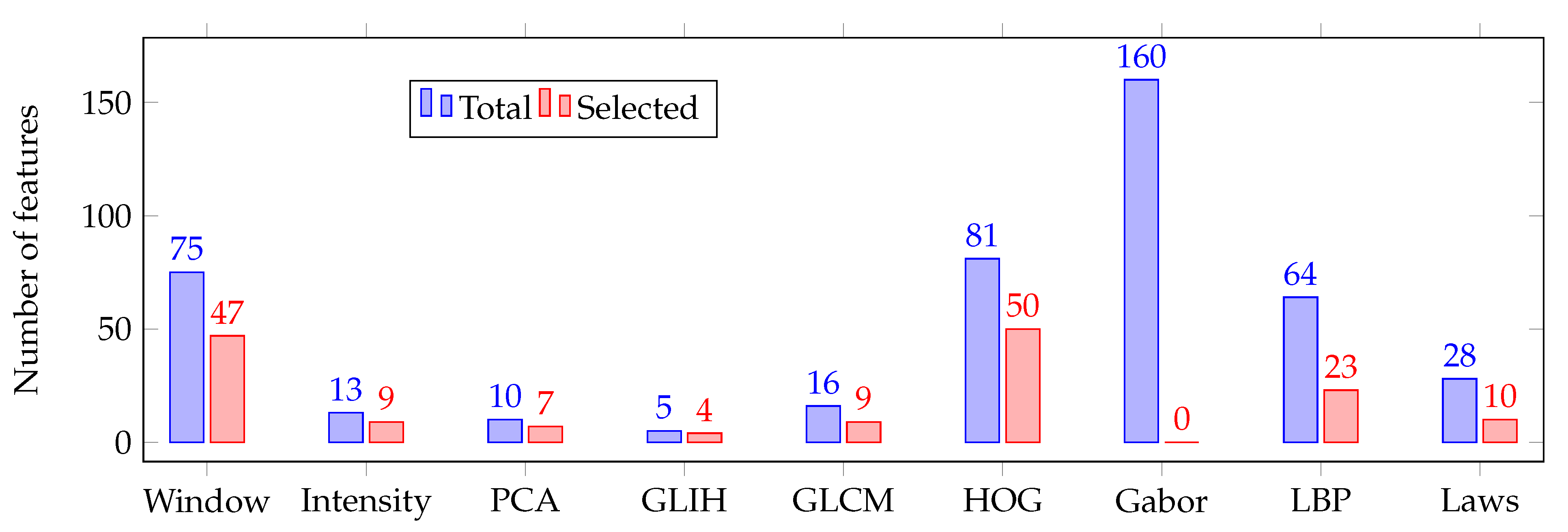
| Texture-Based Features | Principal Component Analysis (PCA) features | 10 |
| Gray-Level Co-occurrence Matrix (GLCM) | 16 | |
| Gabor features | 160 | |
| Local Binary Patterns | 64 | |
| Laws features | 28 | |
| Domain-Related Features | Window features | 75 |
| Intensity-Based Features | Intensity global features | 13 |
| Gray-Level Intensity Histogram (GLIH) | 5 | |
| Histogram of Oriented Gradients (HOG) | 81 |
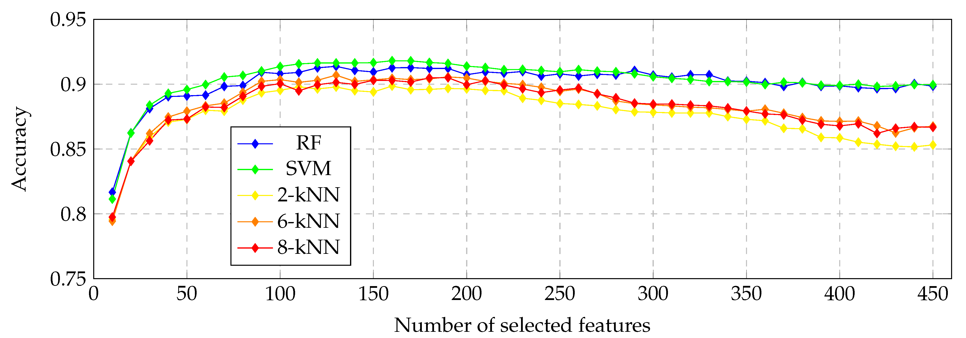
| Number of Features | 20 | 40 | 60 | 80 | 100 | 120 | 140 | 160 | 180 | 200 |
|---|---|---|---|---|---|---|---|---|---|---|
| RF | 0.862 | 0.890 | 0.891 | 0.899 | 0.908 | 0.912 | 0.910 | 0.913 | 0.912 | 0.907 |
| 2-kNN | 0.824 | 0.872 | 0.885 | 0.895 | 0.900 | 0.912 | 0.904 | 0.909 | 0.911 | 0.909 |
| 6-kNN | 0.840 | 0.872 | 0.882 | 0.891 | 0.900 | 0.900 | 0.903 | 0.905 | 0.900 | 0.899 |
| 8-kNN | 0.841 | 0.872 | 0.882 | 0.890 | 0.900 | 0.900 | 0.900 | 0.903 | 0.905 | 0.900 |
| SVM | 0.862 | 0.893 | 0.899 | 0.907 | 0.914 | 0.916 | 0.916 | 0.918 | 0.917 | 0.914 |
| Classifier | RF | 2-kNN | 6-kNN | 8-kNN | SVM |
|---|---|---|---|---|---|
| Number of features | 137 | 182 | 183 | 184 | 159 |
| Accuracy | 0.914 | 0.911 | 0.906 | 0.906 | 0.919 |
| Classification Stage | Post-Processing Stage | ||||||||
|---|---|---|---|---|---|---|---|---|---|
| Patient Class | Identifier | Sensitivity | Specificity | Dice | Jaccard | Sensitivity | Specificity | Dice | Jaccard |
| ERM | Mean | 0.7495 | 0.8944 | 0.6695 | 0.5148 | 0.8251 | 0.919 | 0.7799 | 0.6489 |
| Std. Dev. | ± 0.1648 | ± 0.0652 | ± 0.1101 | ± 0.1403 | ± 0.1545 | ± 0.0544 | ± 0.0924 | ± 0.1277 | |
| Non-ERM | Mean | - | 0.9880 | - | - | - | 0.9901 | - | - |
| Std. Dev. | - | ± 0.0115 | - | - | - | ± 0.0061 | - | - | |
© 2019 by the authors. Licensee MDPI, Basel, Switzerland. This article is an open access article distributed under the terms and conditions of the Creative Commons Attribution (CC BY) license (http://creativecommons.org/licenses/by/4.0/).
Share and Cite
Baamonde, S.; de Moura, J.; Novo, J.; Charlón, P.; Ortega, M. Automatic Identification and Intuitive Map Representation of the Epiretinal Membrane Presence in 3D OCT Volumes. Sensors 2019, 19, 5269. https://doi.org/10.3390/s19235269
Baamonde S, de Moura J, Novo J, Charlón P, Ortega M. Automatic Identification and Intuitive Map Representation of the Epiretinal Membrane Presence in 3D OCT Volumes. Sensors. 2019; 19(23):5269. https://doi.org/10.3390/s19235269
Chicago/Turabian StyleBaamonde, Sergio, Joaquim de Moura, Jorge Novo, Pablo Charlón, and Marcos Ortega. 2019. "Automatic Identification and Intuitive Map Representation of the Epiretinal Membrane Presence in 3D OCT Volumes" Sensors 19, no. 23: 5269. https://doi.org/10.3390/s19235269
APA StyleBaamonde, S., de Moura, J., Novo, J., Charlón, P., & Ortega, M. (2019). Automatic Identification and Intuitive Map Representation of the Epiretinal Membrane Presence in 3D OCT Volumes. Sensors, 19(23), 5269. https://doi.org/10.3390/s19235269