Rigorous Calibration of UAV-Based LiDAR Systems with Refinement of the Boresight Angles Using a Point-to-Plane Approach


Abstract
1. Introduction
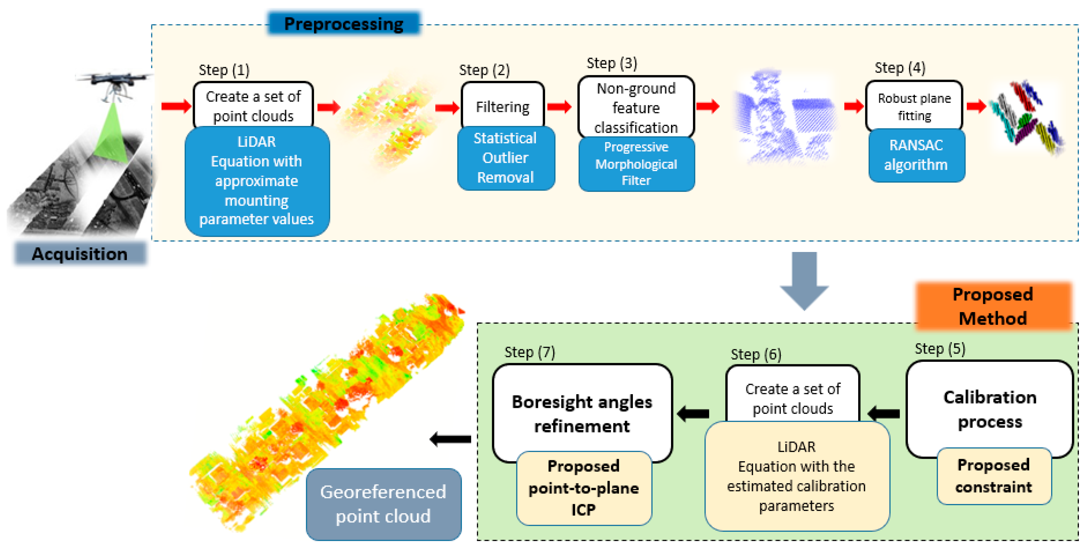
2. Data and Methods
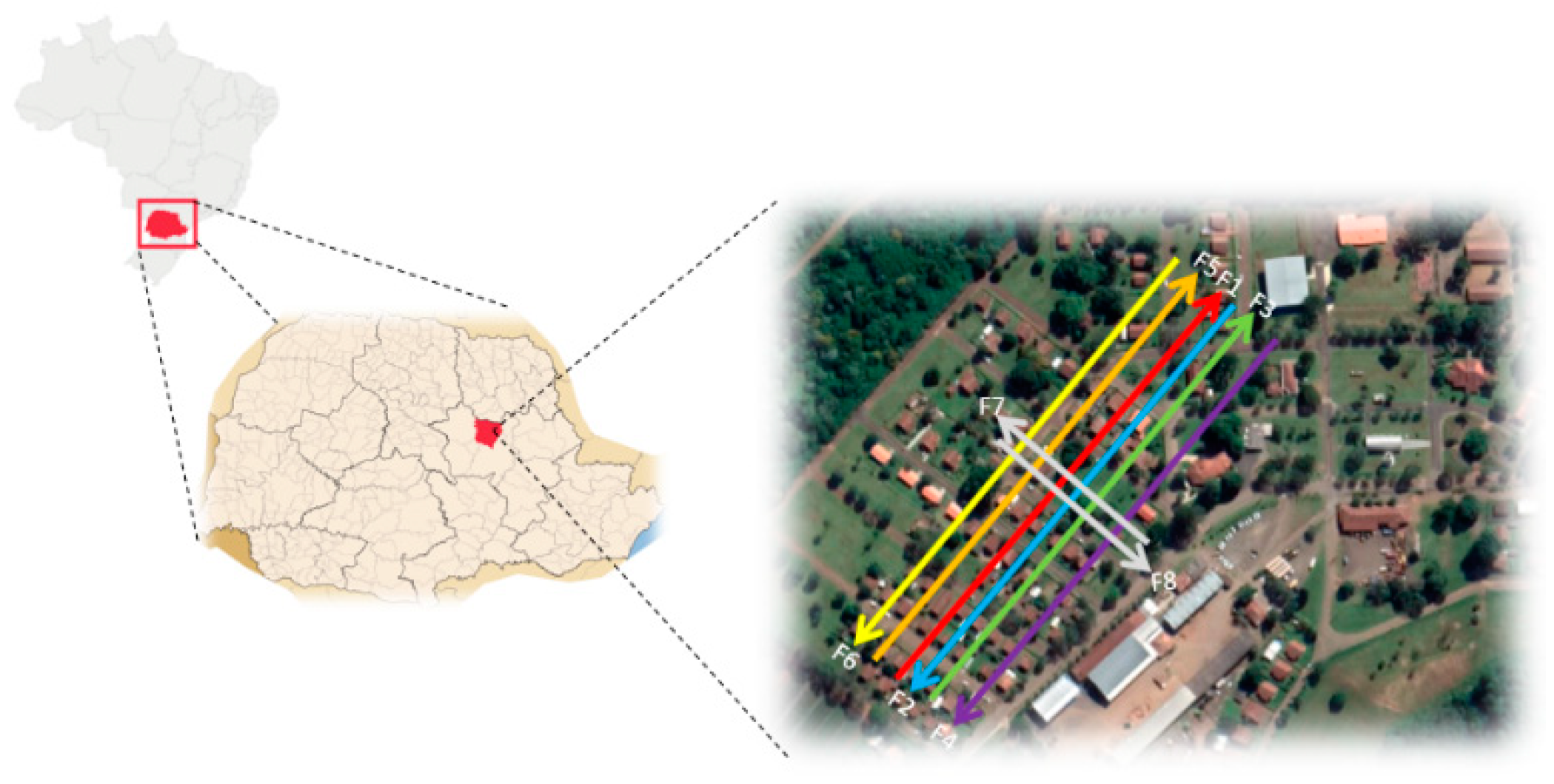
2.1. Study Area and Data Acquisition
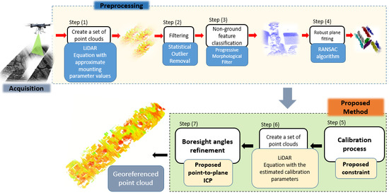
2.2. Method
2.2.1. Point Cloud Generation Using the LiDAR Equation
2.2.2. Point Cloud Processing
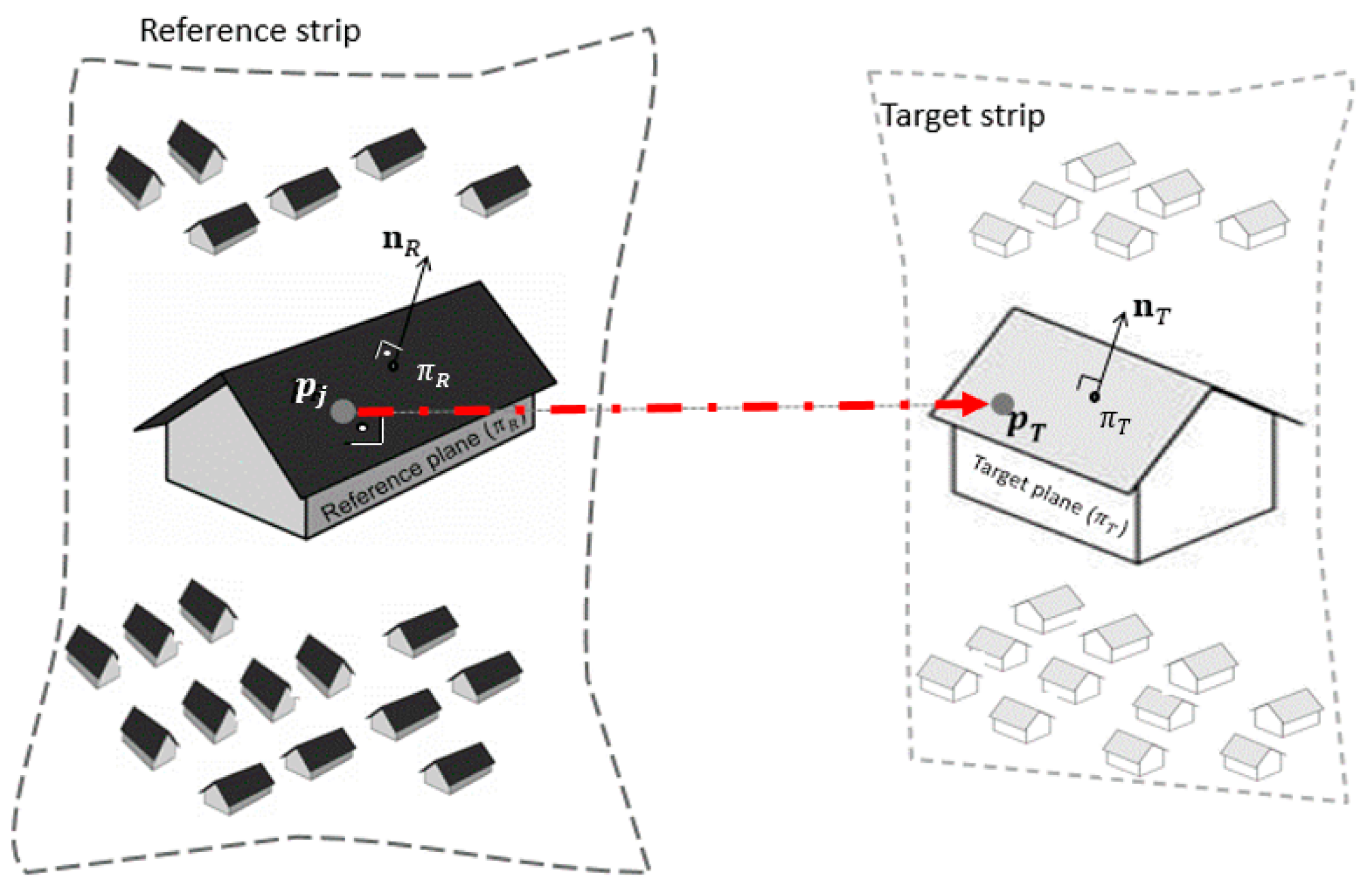
2.2.3. Estimation of the Calibration Parameters Using the Minimum Distance Criteria Constraint
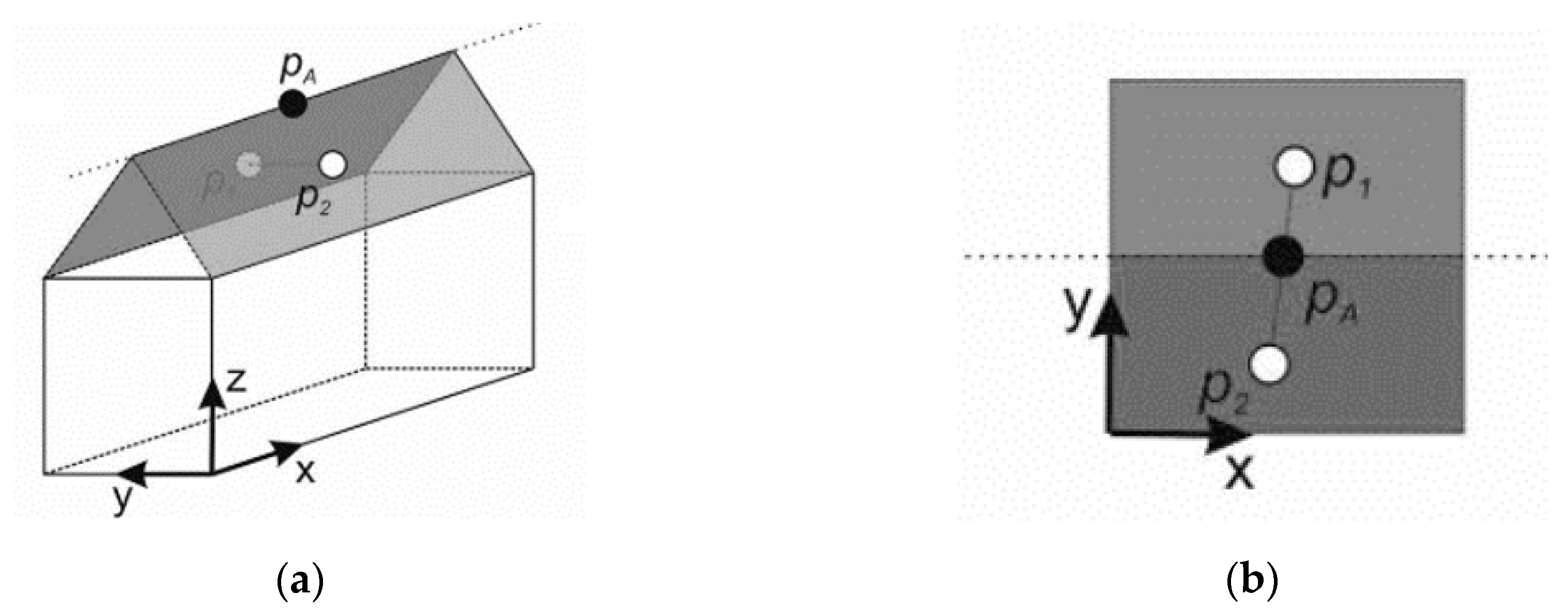
2.2.4. Point-to-Plane Matching Procedure
2.2.5. Boresight Angle Refinement Using a Point-to-Plane Corresponding Model
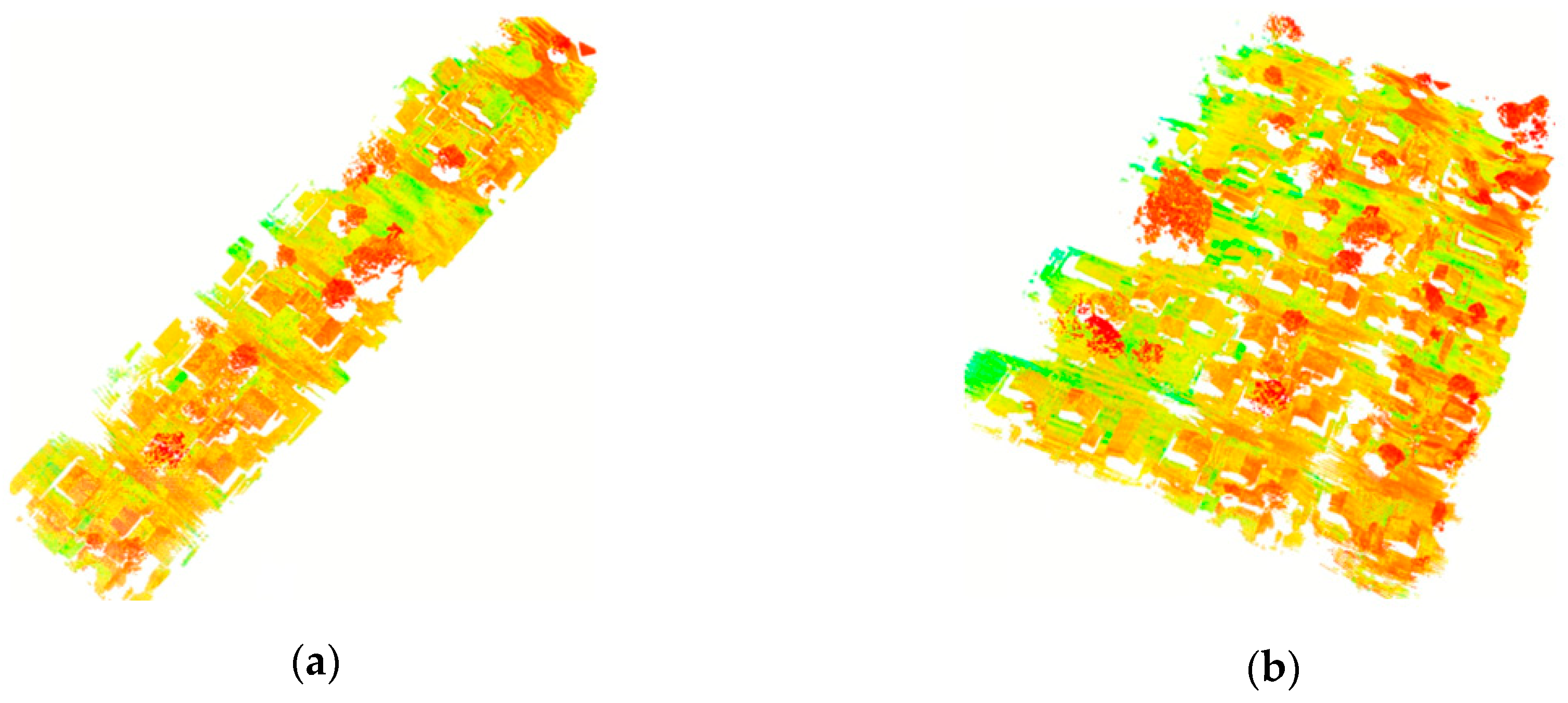
3. Results
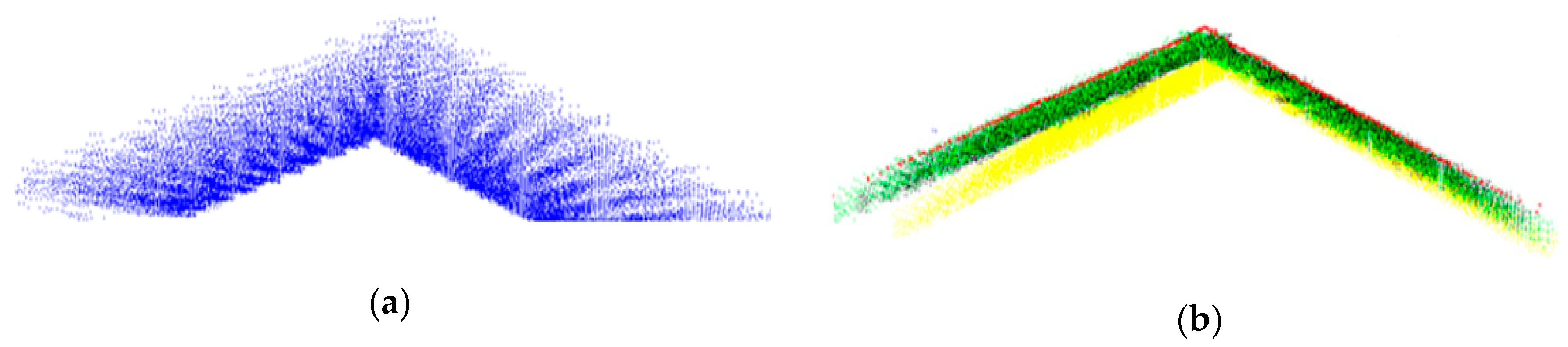
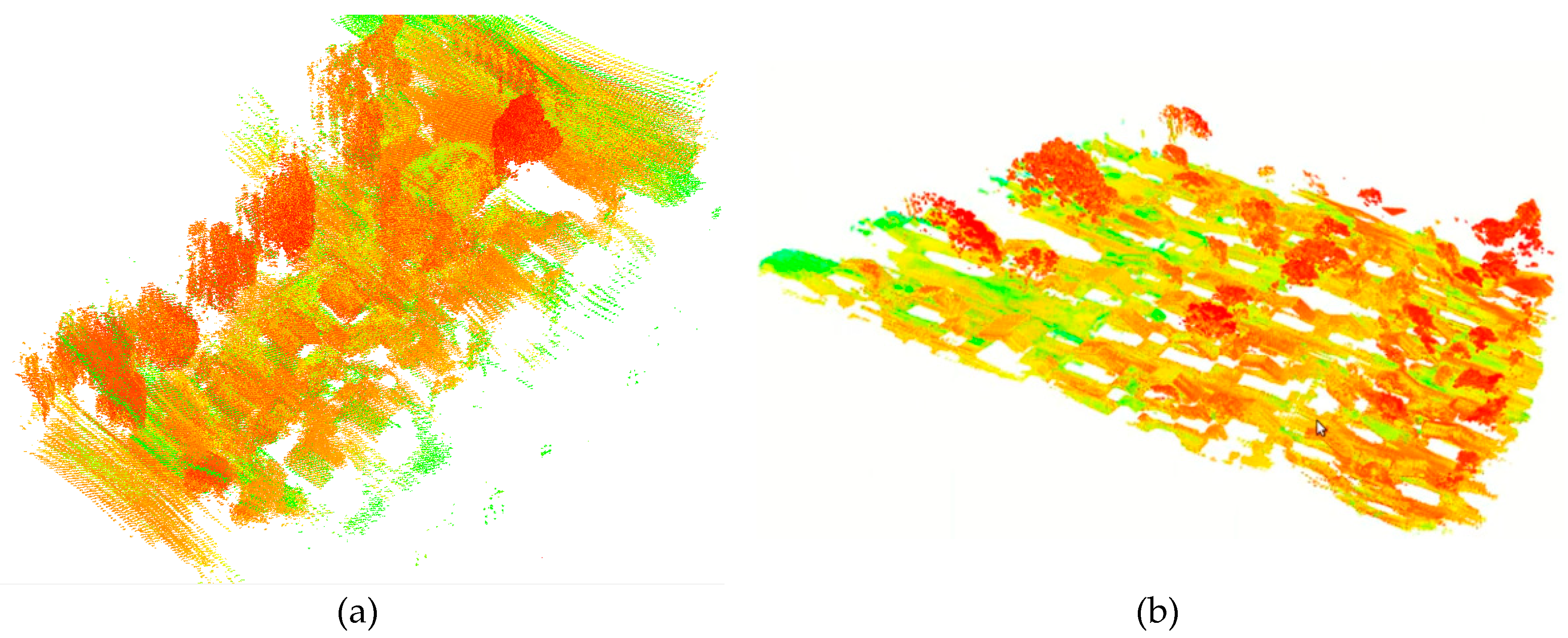
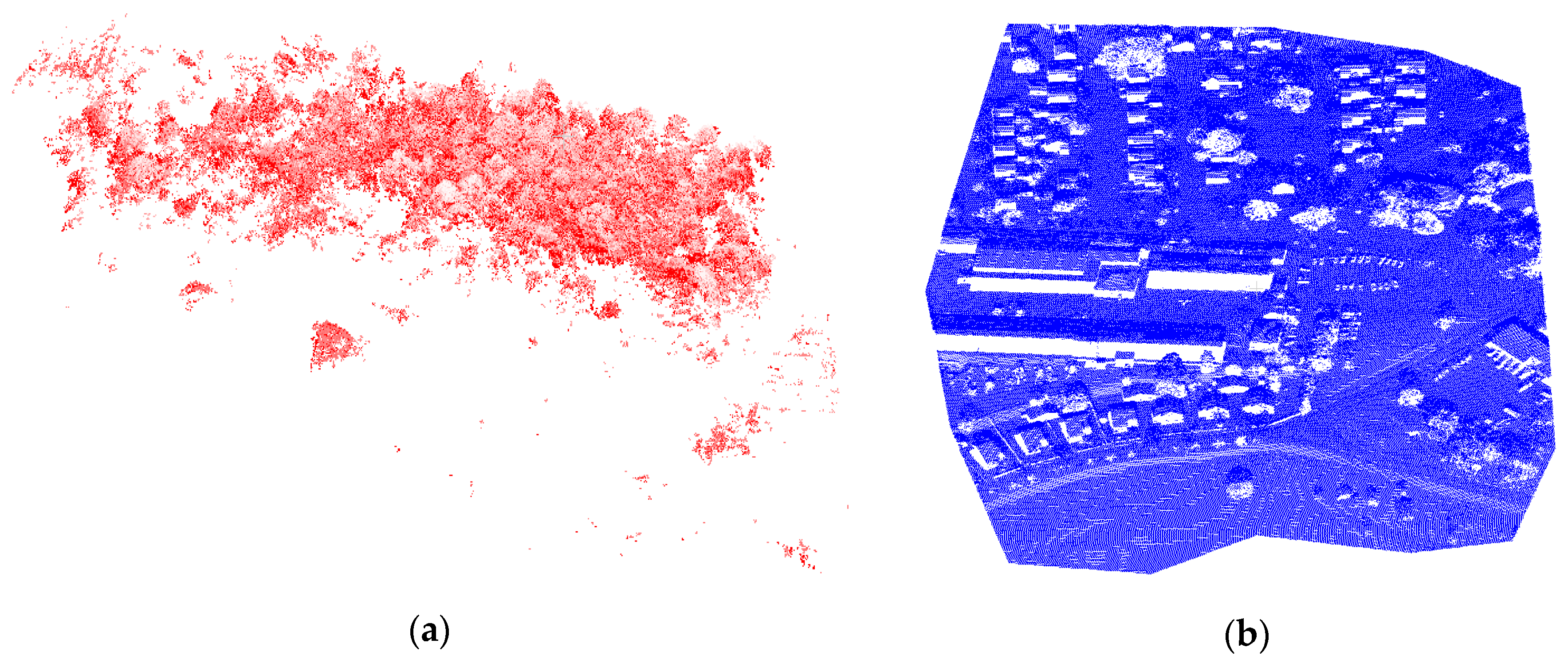
3.1. Gabled Roof Extraction
3.2. Benefits of the Proposed Rigorous Calibration Method
3.2.1. Estimation of the Calibration Parameters
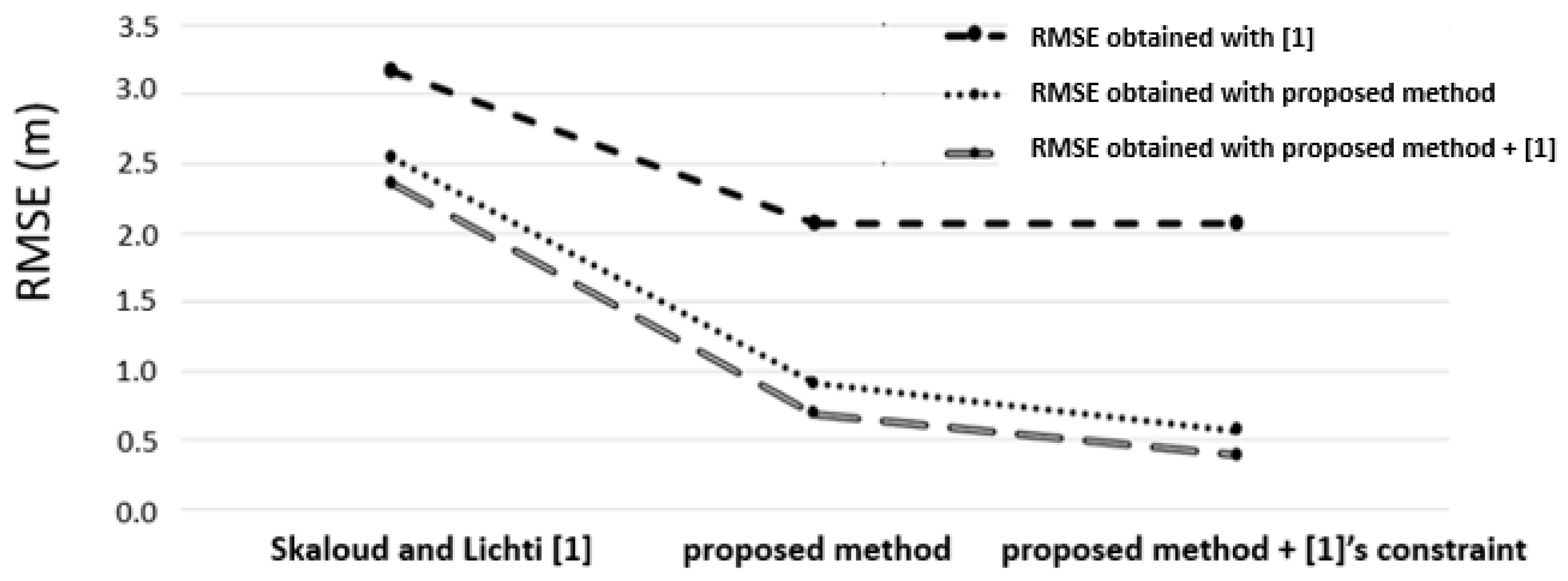
3.2.2. Refinement of the Boresight Angles
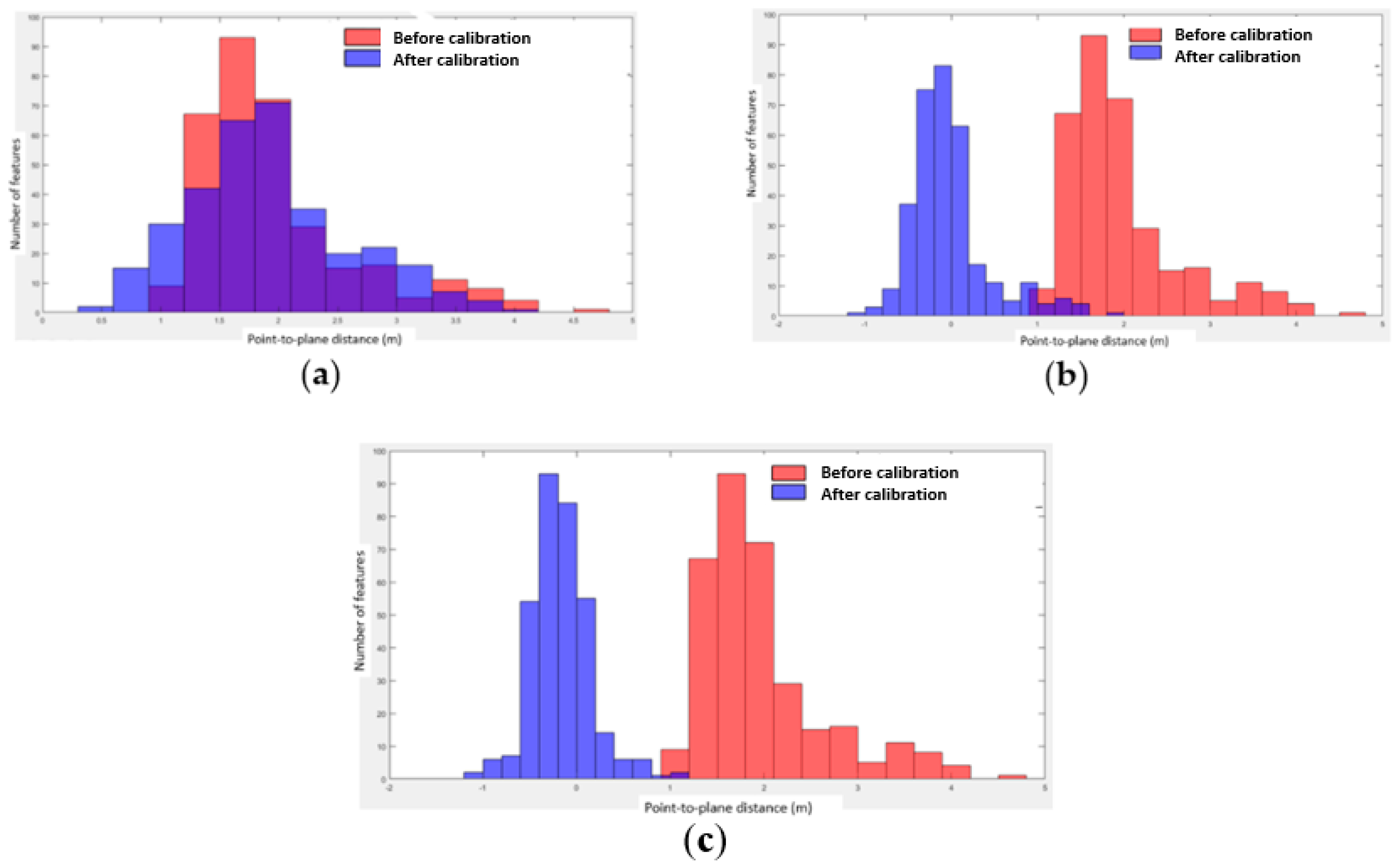
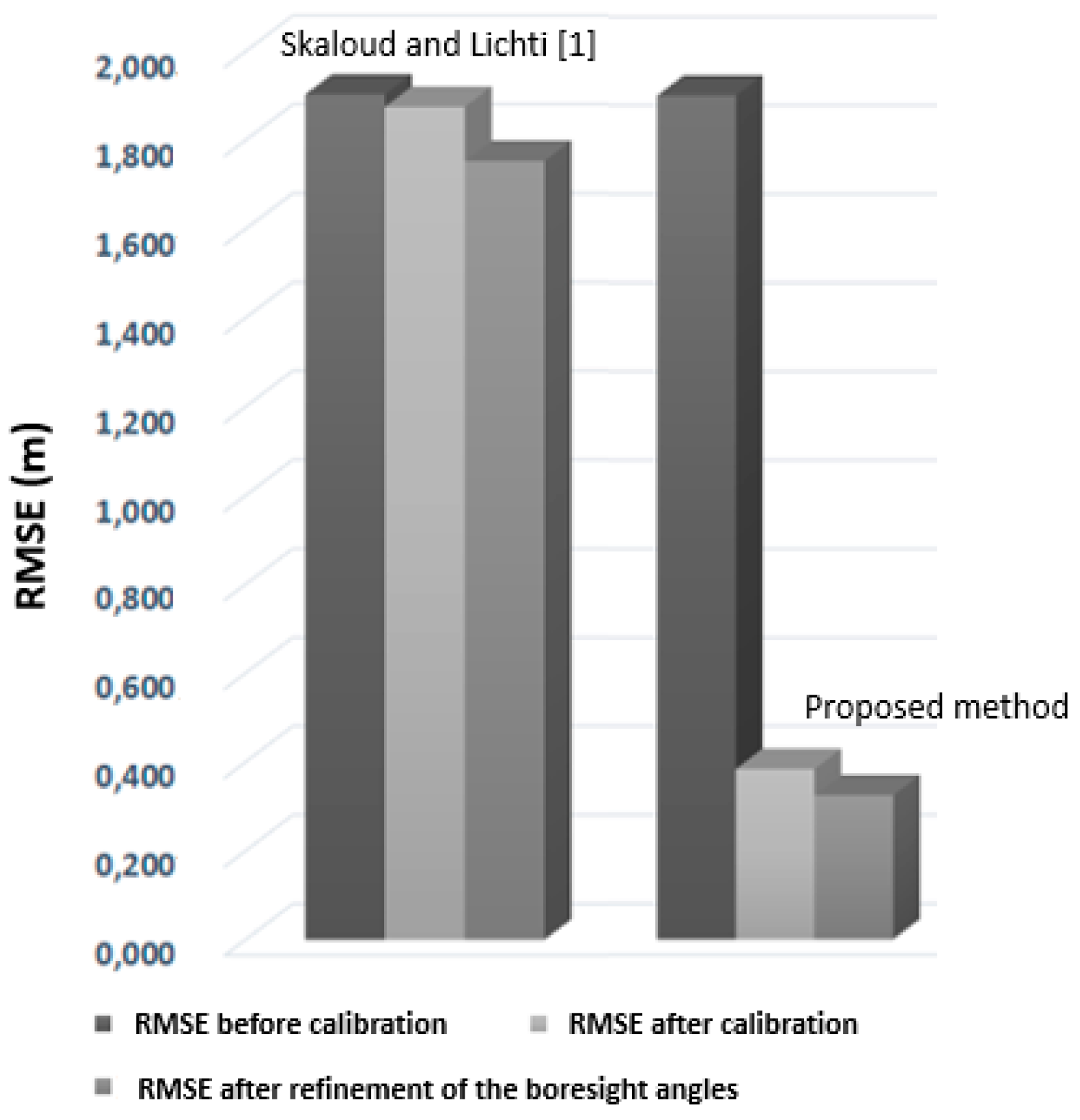
3.2.3. Accuracy Assessment
4. Discussion
4.1. The Influence of the Proposed Constraint
4.2. The Influence of the Proposed Refinement Approach
5. Conclusions
Author Contributions
Funding
Acknowledgments
Conflicts of Interest
References
- Chen, C.F.; Li, Y.; Zhao, N.; Yan, C. Robust interpolation of DEMs from LiDAR-derived elevation data. IEEE Trans. Geosci. Remote Sens. 2018, 56, 1059–1068. [Google Scholar] [CrossRef]
- Lin, Y.; Hyyppä, J.; Jaakkola, A. Mini-UAV-borne LIDAR for fine-scale mapping. IEEE Geosci. Remote Sens. Lett. 2011, 8, 426–430. [Google Scholar] [CrossRef]
- Kwan, M.P.; Ransberger, D.M. LiDAR assisted emergency response: Detection of transport network obstructions caused by major disasters. Comput. Environ. Urban Syst. 2010, 34, 179–188. [Google Scholar] [CrossRef]
- Hou, M.; Li, S.K.; Jiang, L.; Wu, Y.; Hu, Y.; Yang, S.; Zhang, X. A new method of gold foil damage detection in stone carving relics based on multi-temporal 3D LiDAR point clouds. ISPRS Int. J. Geo-Inf. 2016, 5, 60. [Google Scholar] [CrossRef]
- Guo, Q.; Su, T.; Zhao, X.; Wu, F.; Li, Y.; Liu, J.; Chen, L.; Xu, G. An integrated UAV-borne lidar system for 3D habitat mapping in three forest ecosystems across China. Int. J. Remote Sens. 2017, 38, 2954–2972. [Google Scholar] [CrossRef]
- Sankey, T.; Donager, J.; McVay, J.; Sankey, J.B. UAV lidar and hyperspectral fusion for forest monitoring in the southwestern USA. Remote Sens. Environ. 2017, 195, 30–43. [Google Scholar] [CrossRef]
- Wieser, M.; Mandlburger, G.; Hollaus, M.; Otepka, J.; Glira, P.; Pfeifer, N. A case study of UAS borne laser scanning for measurement of tree stem diameter. Remote Sens. 2017, 9, 1154. [Google Scholar] [CrossRef]
- Su, X.; Dong, S.; Liu, S.; Cracknell, A.P.; Zhang, Y.; Wang, X.; Liu, G. Using an unmanned aerial vehicle (UAV) to study wild yak in the highest desert in the world. Int. J. Remote Sens. 2018, 39, 5490–5503. [Google Scholar] [CrossRef]
- Khan, S.; Aragão, L.; Iriarte, J. A UAV–lidar system to map Amazonian rainforest and its ancient landscape transformations. Int. J. Remote Sens. 2017, 38, 2313–2330. [Google Scholar] [CrossRef]
- Teng, G.; Zhou, M.; Li, C.; Wu, H.; Li, W.; Meng, F.; Zhou, C.; Ma, L. Mini-UAV LiDAR for power line inspection. In Proceedings of the International Archives of the Photogrammetry, Remote Sensing and Spatial Information Sciences, Wuhan, China, 18–22 September 2017; pp. 297–300. [Google Scholar]
- Skaloud, J.; Lichti, D. Rigorous approach to bore-sight self-calibration in airborne laser scanning. ISPRS J. Photogram. Remote Sens. 2006, 61, 47–59. [Google Scholar] [CrossRef]
- Crombaghs, M.J.E.; Brugelmann, R.; de Min, E.J. On the Adjustment of Overlapping Strips of Laser Altimeter Height Data. In Proceedings of the International Archives of the Photogrammetry, Remote Sensing and Spatial Information Sciences, Amsterdam, The Netherlands, 16–22 July 2000; pp. 230–237. [Google Scholar]
- Glira, P.; Pfeifer, N.; Mandlburger, G. Rigorous strip adjustment of UAV-based laserscanning data including time-dependent correction of trajectory errors. Photogramm. Eng. Remote Sens. 2016, 82, 945–954. [Google Scholar] [CrossRef]
- Fritsch, G.; Kilian, J. Filtering and calibration of laser scanner measurements. In Proceedings of the International Archives of Photogrammetry and Remote Sensing, Munich, Germany, 5–9 September 1994; pp. 227–234. [Google Scholar]
- Kager, H.; Kraus, K. Height discrepancies between overlapping laser scanner strips. In Proceedings of the Optical 3D Measurements Techniques V, Vienna, Austria, 1–4 October 2001; pp. 227–234. [Google Scholar]
- Vosselman, G.; Maas, H.-G. Adjustment and filtering of raw laser altimetry data. In Proceedings of the OEEPE Workshop on Airborne Laser Systems and Interferometric SAR for Detailed Digital Elevation Models, Stockholm, Sweden, 1–3 March 2001; OEEPE Official Publication no. 40. pp. 62–72. [Google Scholar]
- Maas, H.-G. Methods for measuring height and planimetry discrepancies in airborne laserscanner data. Photogramm. Eng. Remote. Sens. 2002, 68, 933–940. [Google Scholar]
- Hodgson, M.E.; Bresnahan, P. Accuracy of Airborne Lidar-Derived Elevation: Empirical Assessment and Error Budget. Photogramm. Eng. Remote Sens. 2004, 70, 331–339. [Google Scholar] [CrossRef]
- Bretar, F.; Pierrot-Deseilligny, M.; Roux, M. Solving the strip adjustment problem of 3D airborne LiDAR data. In Proceedings of the IEEE IGARSS’04, Anchorage, Alaska, 20–24 September 2004. [Google Scholar]
- Csanyi, N.; Toth, C.K. Improvement of LiDAR data accuracy using LiDAR-Specific ground targets. Photogramm. Eng. Remote Sens. 2007, 73, 385–396. [Google Scholar] [CrossRef]
- Ressl, C.; Mandlburgera, G.; Pfeifer, N. Investigating adjustment of airborne laser scanning strips without usage of GNSS/IMU trajectory data. In Proceedings of the ISPRS Workshop, Paris, France, 1–2 September 2009; pp. 195–200. [Google Scholar]
- Latypov, D. Estimating relative LiDAR accuracy information from overlapping flight lines. ISPRS J. Photogramm. Remote Sens. 2002, 56, 236–245. [Google Scholar] [CrossRef]
- Vosselman, G. Strip offset estimation using linear features. In Proceedings of the 3rd International Workshop on Mapping Geo-Surfical Processes Using Laser Altimetry, Columbus, OH, USA, 7–9 October 2002; pp. 1–9. [Google Scholar]
- Filin, S.; Vosselman, G. Adjustment of airborne laser altimetry strips. Int. Arch. Photogramm. Remote Sens. Spat. Inform. Sci. 2004, 35, 285–289. [Google Scholar]
- Van der Sande, C.; Soudarissanane, S.; Khoshelham, K. Assessment of relative accuracy of AHN-2 laser scanning data using planar features. Sensors 2010, 10, 8198–8214. [Google Scholar] [CrossRef]
- Besl, P.; Mckay, N.D. A method for registration of 3–D shapes. IEEE Trans. Pattern Anal. Mach. Intell. 1992, 14, 239–256. [Google Scholar] [CrossRef]
- Chen, Y.; Medioni, G. Object modelling by registration of multiple range images. Image Vision Comput. 1992, 10, 145–155. [Google Scholar] [CrossRef]
- Filin, S. Recovery of systematic biases in laser altimetry data using natural surfaces. Photogramm. Eng. Remote Sens. 2003, 69, 1235–1242. [Google Scholar] [CrossRef]
- Habib, A.; Bang, K.I.; Kersting, A.P.; Chow, J. Alternative methodologies for LiDAR system calibration. Remote Sens. 2010, 874–907. [Google Scholar] [CrossRef]
- Glira, P.; Pfeifer, N.; Briese, C.; Ressl, C. A correspondence framework for ALS strip adjustment based on variants of the ICP algorithm. Photogram. Fernerk. Geoinform. 2015, 4, 275–289. [Google Scholar] [CrossRef]
- Kilian, J.; Haala, N.; Englich, M. Capture and evaluation of airborne laser scanner data. In Proceedings of the International Archives of the Photogrammetry, Remote Sensing and Spatial Information Sciences, Vienna, Austria, 12–18 July 1996; pp. 383–388. [Google Scholar]
- Kersting, A.P.; Habib, A.; Bang, K.I.; Skaloud, J. Automated approach for rigorous light detection and ranging system calibration without preprocessing and strict terrain coverage requirements. Optical Eng. 2012, 51, 100–120. [Google Scholar] [CrossRef]
- Ravi, R.; Shamseldin, T.; Elbahnasawy, M.; Lin, Y.J.; Habib, A. Bias Impact Analysis and Calibration of UAV-Based Mobile LiDAR System with Spinning Multi-Beam Laser Scanner. Appl. Sci. 2018, 8, 297. [Google Scholar] [CrossRef]
- Li, Z.; Tan, J.; Liu, H. Rigorous Boresight Self-Calibration of Mobile and UAV LiDAR Scanning Systems by Strip Adjustment. Remote Sens. 2019, 11, 442. [Google Scholar] [CrossRef]
- Rusinkiewicz., S.; Levoy, M. Efficient variants of the ICP algorithm. In Proceedings of the Third International Conference on 3–D Digital Imaging and Modeling IEEE, Quebec City, QC, Canada, 28 May–1 June 2001; pp. 145–152. [Google Scholar]
- Zhang, X.; Gao, R.; Sun, Q.; Cheng, J. An automated rectification method for unmanned aerial vehicle lidar point cloud data based on laser intensity. Remote Sens. 2019, 11, 811. [Google Scholar] [CrossRef]
- Velodyne. Velodyne VLP-16 User Manual. 2016. Available online: http://velodynelidar.com/docs/manuals/63243%20Rev%20B%20User%20Manual%20and%20Programming%20Guide,VLP-16.pdf (accessed on 17 September 2019).
- Applanix, APX-15 UAV, Single Board GNSS-Inertial Solution. 2016. Available online: https://www.applanix.com/downloads/products/specs/APX15_DS_NEW_0408_YW.pdf (accessed on 10 November 2018).
- Rusu, R.B.; Marton, Z.C.; Blodow, N.; Dolha, M.; Beetz, M. Towards 3D Point Cloud Based Object Maps for Household Environments. Robot. Auton. Syst. 2008, 56, 927–941. [Google Scholar] [CrossRef]
- Zhang, K.Q.; Chen, S.C.; Whitman, D.; Shyu, M.L.; Yan, J.H.; Zhang, C.C. A progressive morphological filter for removing non-ground measurements from airborne LiDAR data. IEEE Trans. Geosci. Remote Sens. 2003, 41, 872–882. [Google Scholar] [CrossRef]
- Fischler, M.A.; Bolles, R.C. Random sample consensus: A paradigm for model fitting with applications to image analysis and automated cartography. Comm. ACM 1981, 24, 42–65. [Google Scholar] [CrossRef]
- Rabbani, T.; van den Heuvel, F.; Vosselman, G. Segmentation of point clouds using smoothness constraint. Int. Arch. Photogramm. Remote Sens. Spat. Inform. Sci. 2006, 36, 248–253. [Google Scholar]
- Arya, S.; Mount, D.M.; Netanyahu, N.S.; Silverman, R.; Wu, A.Y. An optimal algorithm for approximate nearest neighbor searching fixed dimensions. J. ACM 1998, 45, 891–923. [Google Scholar] [CrossRef]
- Hoppe, H.; DeRose, T.; Duchamp, T.; McDonald, J.; Stuetzle, W. Surface reconstruction from unorganized points. In Proceedings of ACM SIGGRAPH ’92; ACM Press: New York, NY, USA, 1992; pp. 71–782. [Google Scholar]


| Pair of Strips | Overlap (%) | Flight Line Direction |
|---|---|---|
| F1-F2 | 100 | North–South |
| F2-F3 | 70 | North–South |
| F3-F4 | 50 | North–South |
| F2-F4 | 20 | North–North |
| F1-F5 | 70 | North–North |
| F5-F6 | 50 | North–South |
| F1-F6 | 20 | North–South |
| F7-F8 | 100 | West–East |
| PPF | ||
| Cell size = 1 m; base of the exponential window = 2 cells; increment step for windows = 2 m; slope = 5%; maximum threshold = 10 m | ||
| RANSAC | ||
| Minimum number of inliers = 15; tolerance = 10 cm; number of consensus = 10; angle minimum of the plane = 10 degrees, maximum angle of the plane = 80 degrees | ||
| RGF | ||
| Minimum size = 40; maximum size = 500; angular threshold = 1 degree; outlier removal ratio = 4 m | ||
| Scenario A | ||
| Scenario B | ||
| Scenario C | ||
| Calibration Parameters | Scenario A | Scenario B | Scenario C |
|---|---|---|---|
| (°) | 0.01870.0049 | 0.02850.0082 | –0.00120.0061 |
| (°) | –0.01550.0037 | 0.01080.0099 | 0.05070.0205 |
| (°) | 0.00080.0165 | 0.01350.0038 | 0.04460.0177 |
| Method | Average of the Errors (%) |
|---|---|
| [11] | 80 |
| Proposed method | 20 |
© 2019 by the authors. Licensee MDPI, Basel, Switzerland. This article is an open access article distributed under the terms and conditions of the Creative Commons Attribution (CC BY) license (http://creativecommons.org/licenses/by/4.0/).
Share and Cite
de Oliveira Junior, E.M.; dos Santos, D.R. Rigorous Calibration of UAV-Based LiDAR Systems with Refinement of the Boresight Angles Using a Point-to-Plane Approach. Sensors 2019, 19, 5224. https://doi.org/10.3390/s19235224
de Oliveira Junior EM, dos Santos DR. Rigorous Calibration of UAV-Based LiDAR Systems with Refinement of the Boresight Angles Using a Point-to-Plane Approach. Sensors. 2019; 19(23):5224. https://doi.org/10.3390/s19235224
Chicago/Turabian Stylede Oliveira Junior, Elizeu Martins, and Daniel Rodrigues dos Santos. 2019. "Rigorous Calibration of UAV-Based LiDAR Systems with Refinement of the Boresight Angles Using a Point-to-Plane Approach" Sensors 19, no. 23: 5224. https://doi.org/10.3390/s19235224
APA Stylede Oliveira Junior, E. M., & dos Santos, D. R. (2019). Rigorous Calibration of UAV-Based LiDAR Systems with Refinement of the Boresight Angles Using a Point-to-Plane Approach. Sensors, 19(23), 5224. https://doi.org/10.3390/s19235224