A Semi-Automated Object-Based Gully Networks Detection Using Different Machine Learning Models: A Case Study of Bowen Catchment, Queensland, Australia

 ,
,  ,
, 
 and
and 
Abstract
1. Introduction
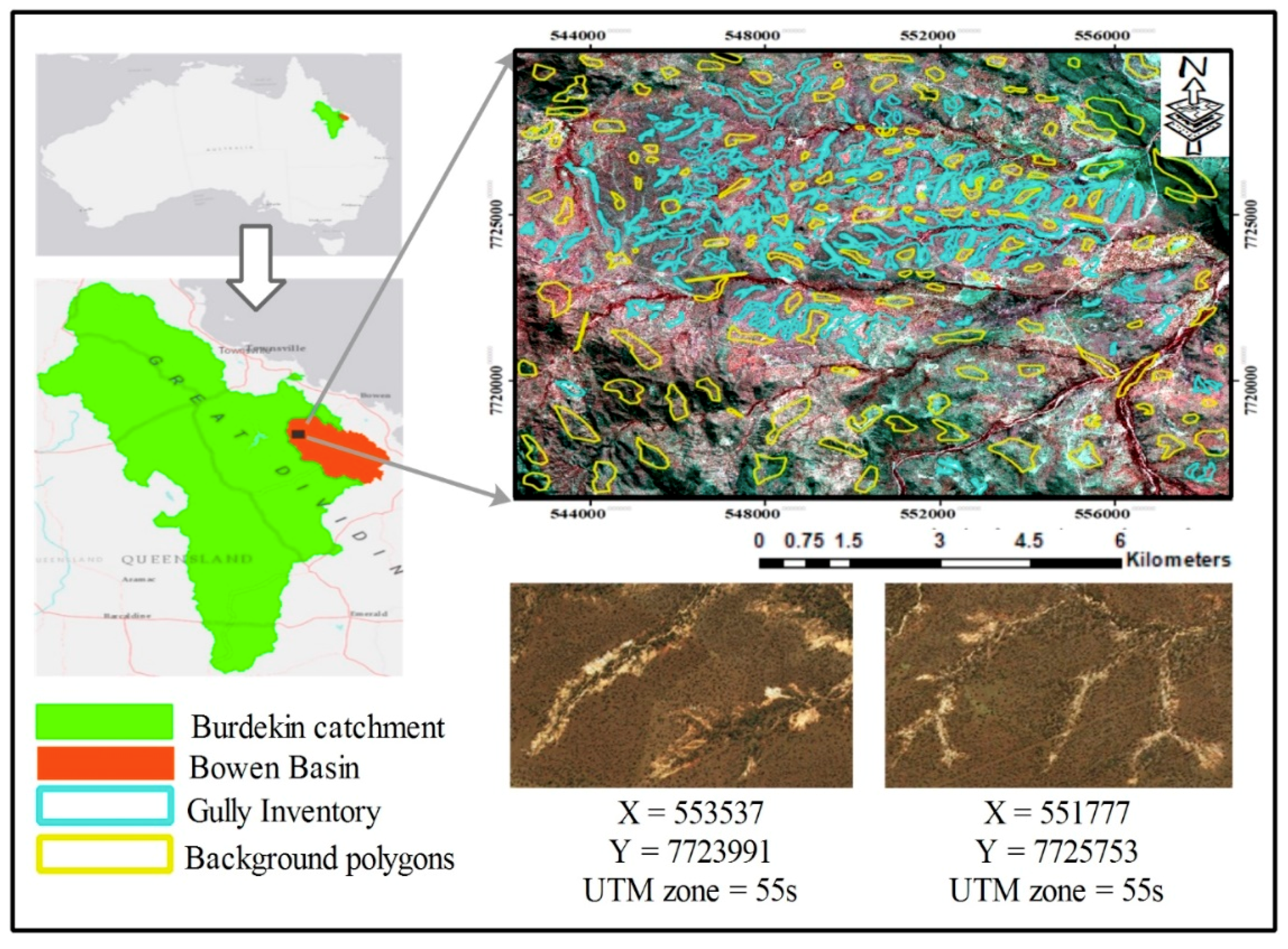
2. Study Area
3. Methodology
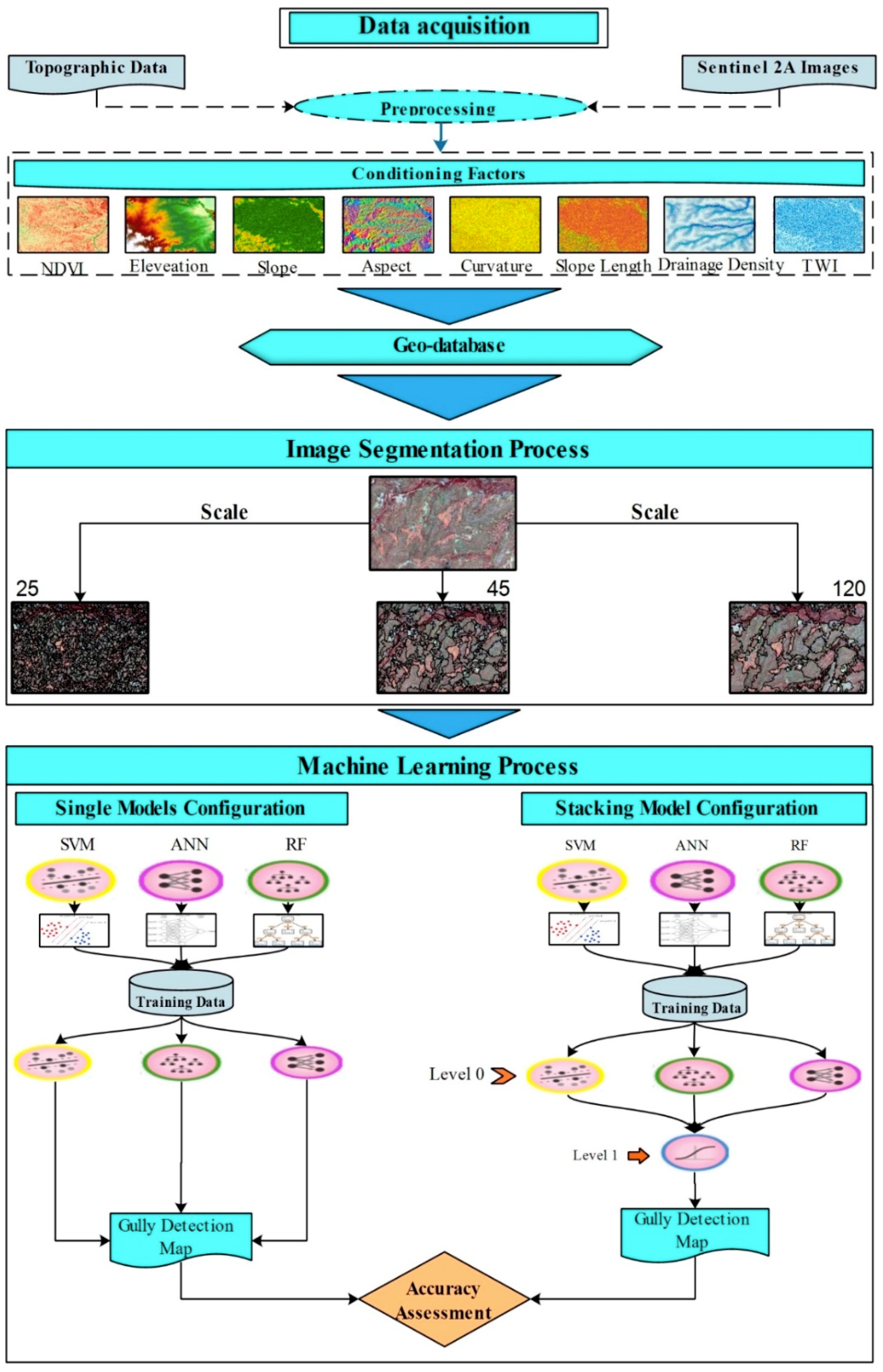
3.1. Overall Workflow
- Preparing Sentinel 2A images, spectral index, and conditioning factors for modelling
- Preparing training and validation for recognition of gully features by
- Running image segmentation using the ESP2 tool
- Assessing the accuracy of produced objects using different scale values
- Selecting the optimal scale value
- Training and testing the ML models based on a gully inventory map
- Selecting the best ML model based on the resulting maps
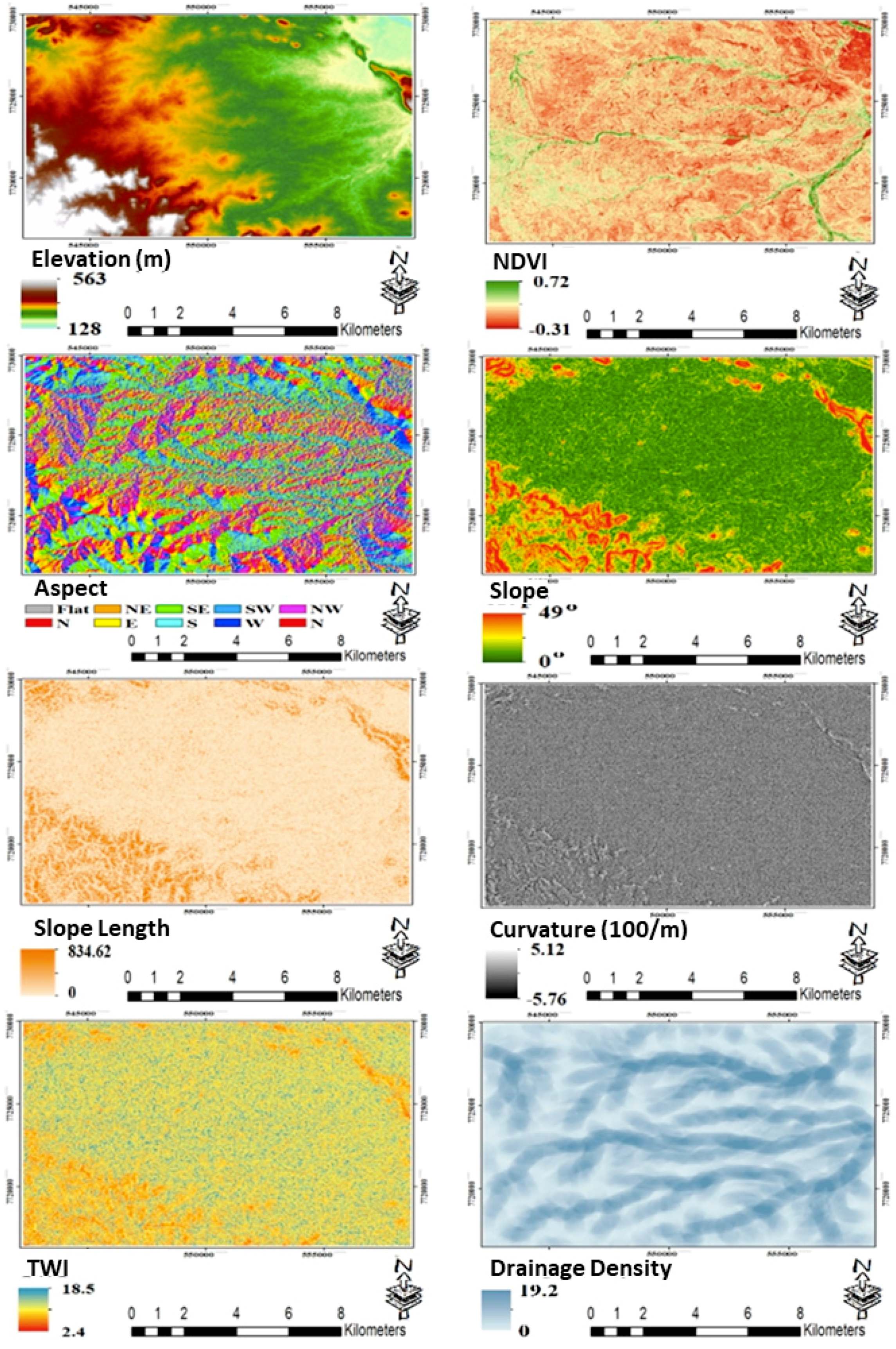
3.2. Datasets
3.3. Geographic Object-Based Image Analysis (GEOBIA)
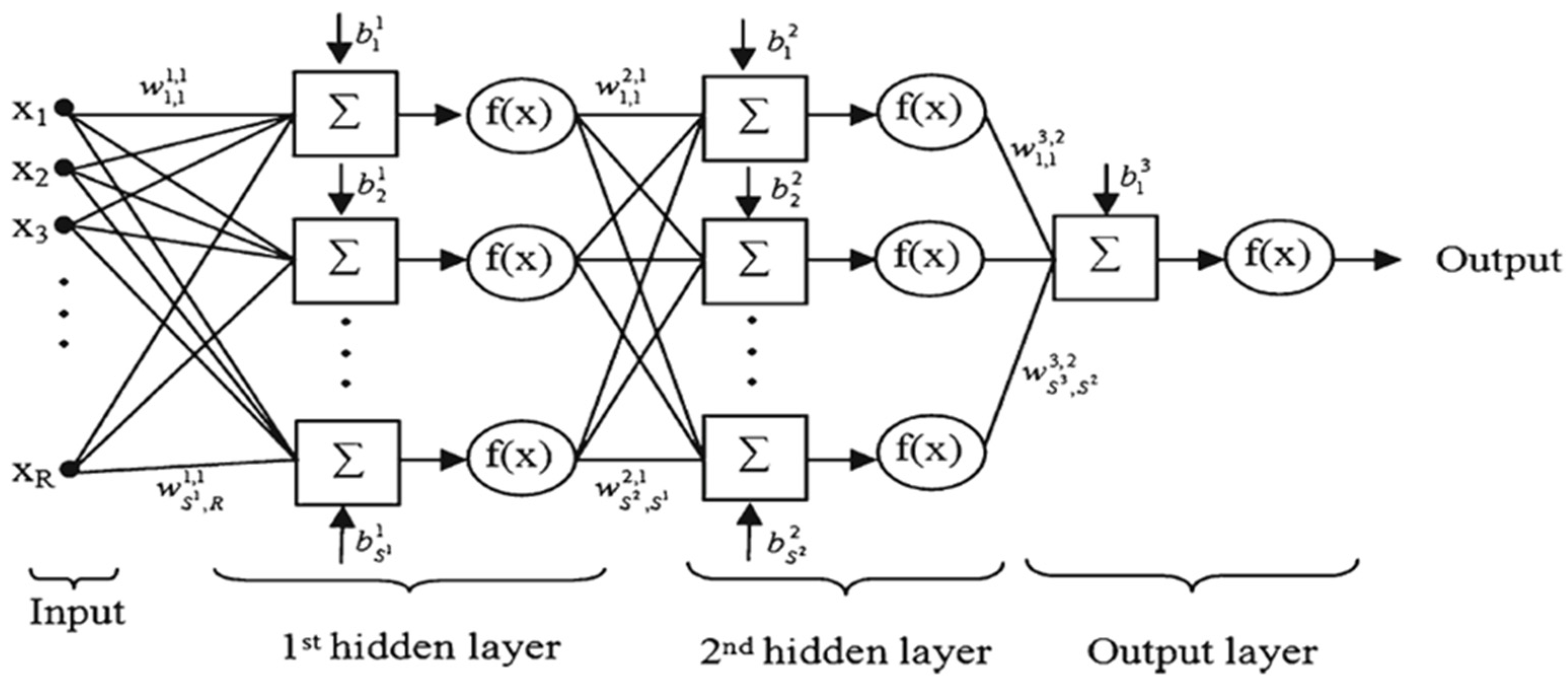
3.4. Artificial Neural Network (ANN)
3.5. Random Forest (RF)
3.6. Support Vector Machine (SVM)
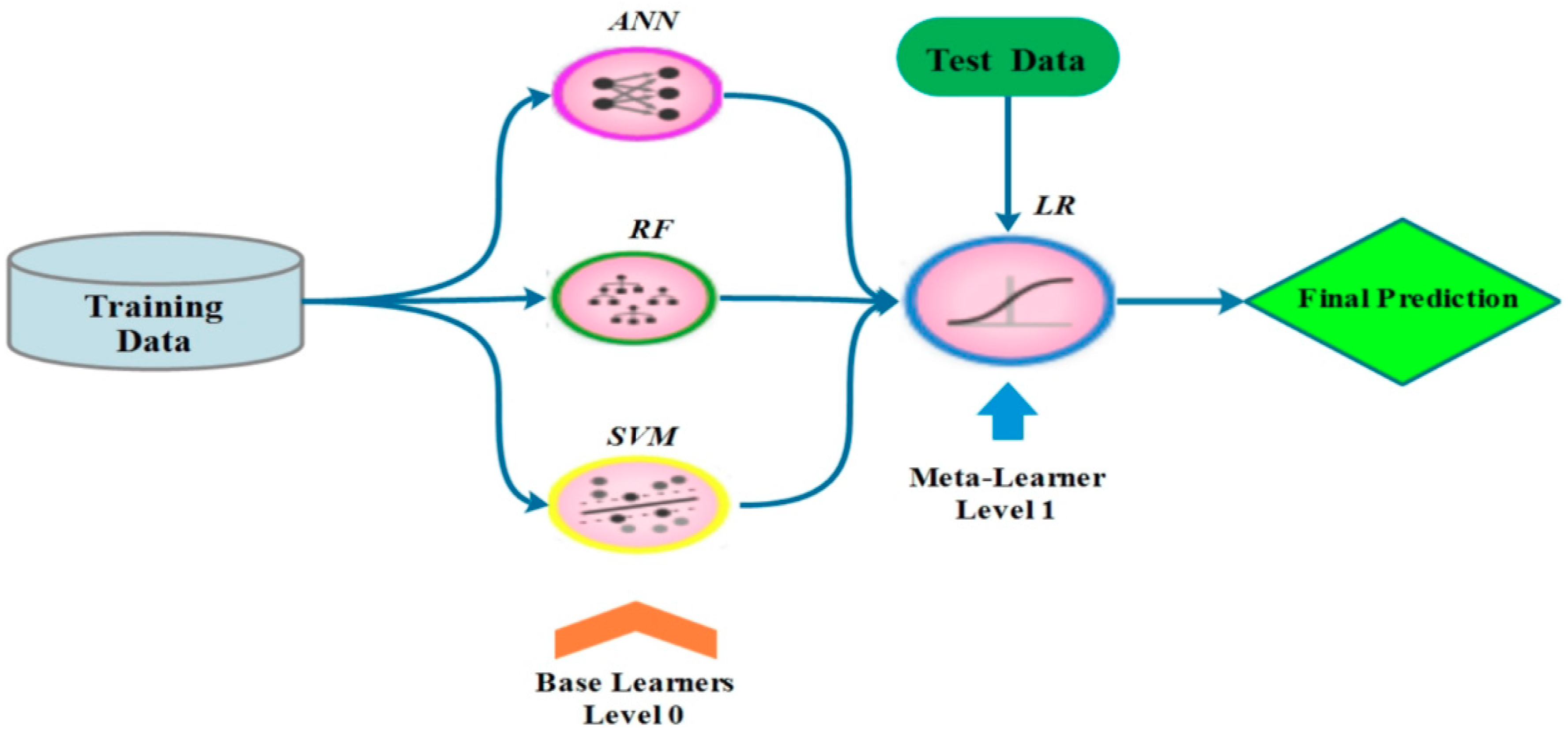
3.7. Stacking
- Specify and configure heterogeneous ML models
- Training the learners at level 0 using the training dataset and perform k-fold cross-validation on each of the ML models to collect the cross-validated predicted values of models
- Building an N × M matrix, in which N is cross-validated predicted values from each of the models and M is the learners. This matrix is named “level 1” data
- Fitting a meta-learner model to level-1 data matrix
- Make prediction using trained meta-learner based on the test data
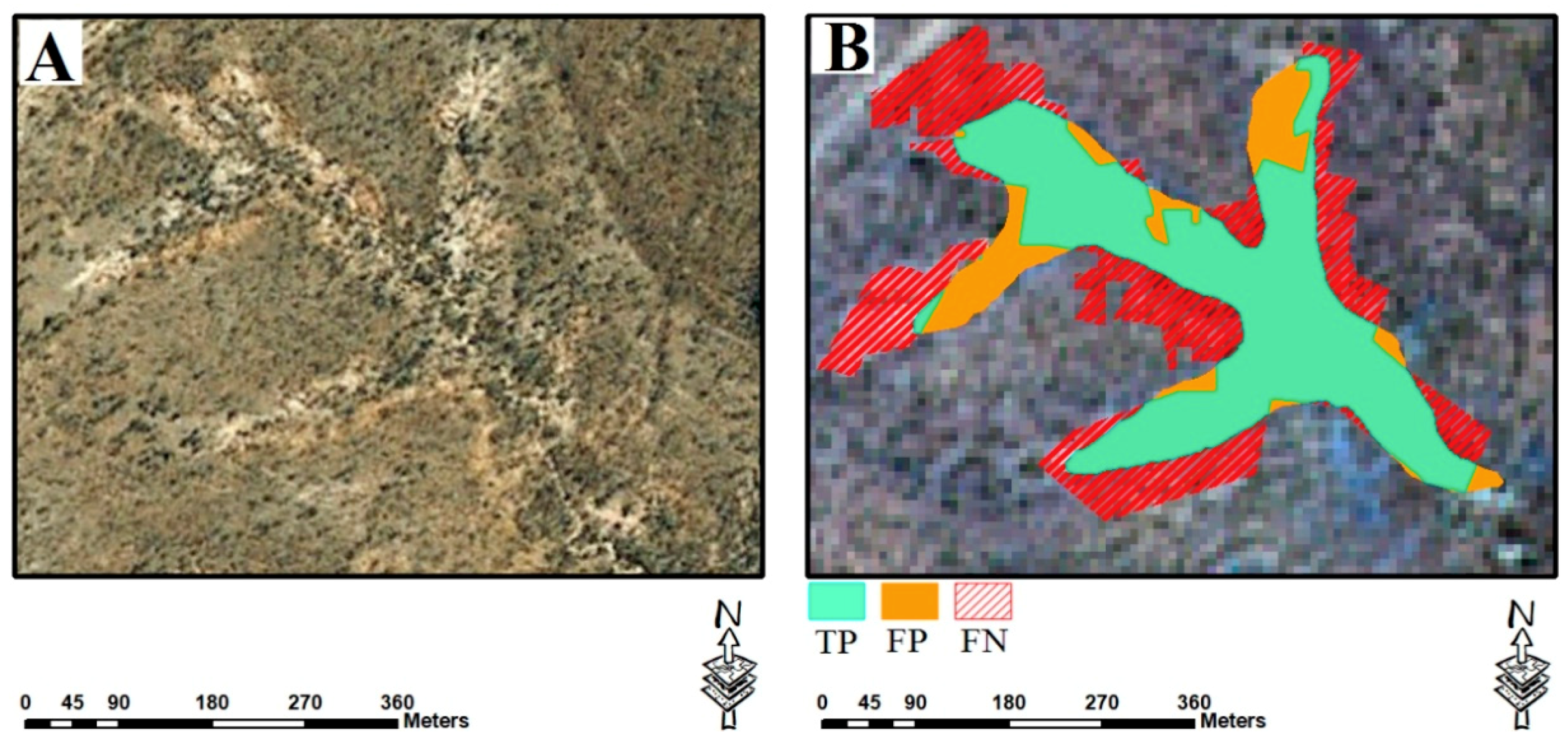
3.8. Accuracy Assessments
4. Results
4.1. Image Segmentation
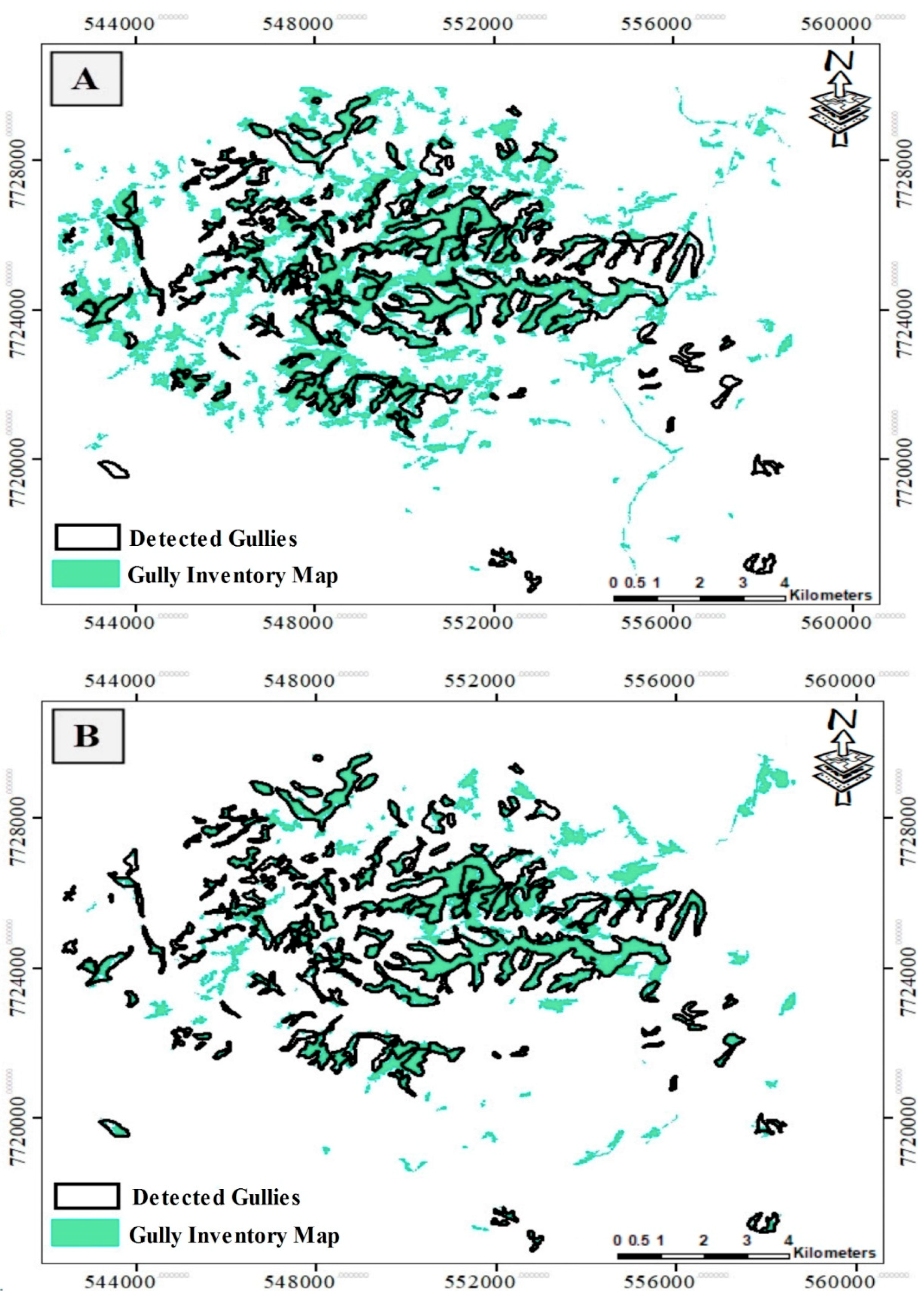
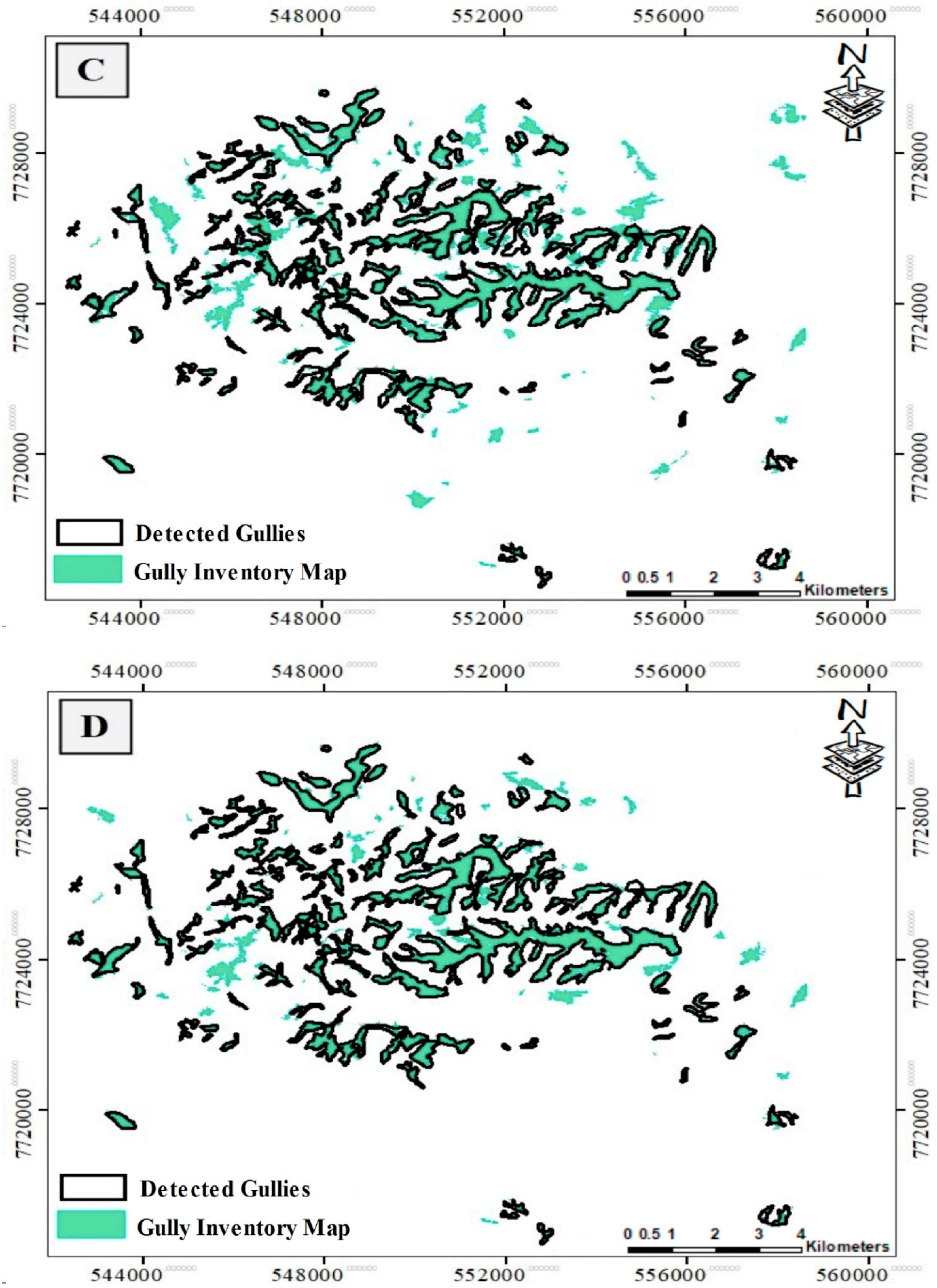
4.2. Gully Network Detection Using ML and Stacking Models
5. Discussion
6. Conclusions and Future Work
Author Contributions
Funding
Acknowledgments
Conflicts of Interest
References
- Mekonnen, M.; Keesstra, S.D.; Baartman, J.E.; Stroosnijder, L.; Maroulis, J. Reducing sediment connectivity through man-made and natural sediment sinks in the Minizr catchment, Northwest Ethiopia. Land Degrad. Dev. 2017, 28, 708–717. [Google Scholar] [CrossRef]
- Tien Bui, D.; Shirzadi, A.; Shahabi, H.; Chapi, K.; Omidavr, E.; Pham, B.T.; Talebpour Asl, D.; Khaledian, H.; Pradhan, B.; Panahi, M.; et al. A Novel Ensemble Artificial Intelligence Approach for Gully Erosion Mapping in a Semi-Arid Watershed (Iran). Sensors 2019, 19, 2444. [Google Scholar] [CrossRef] [PubMed]
- Valentin, C.; Poesen, J.; Li, Y. Gully erosion: Impacts, factors and control. Catena 2005, 63, 132–153. [Google Scholar] [CrossRef]
- Nyssen, J.; Poesen, J.; Moeyersons, J.; Luyten, E.; Veyret-Picot, M.; Deckers, J.; Haile, M.; Govers, G. Impact of road building on gully erosion risk: A case study from the northern Ethiopian highlands. Earth Surf. Process. Landf. J. Br. Geomorphol. Res. Group 2002, 27, 1267–1283. [Google Scholar] [CrossRef]
- Poesen, J.; Nachtergaele, J.; Verstraeten, G.; Valentin, C. Gully erosion and environmental change: Importance and research needs. Catena 2003, 50, 91–133. [Google Scholar] [CrossRef]
- Li, H.; Cruse, R.M.; Bingner, R.L.; Gesch, K.R.; Zhang, X. Evaluating ephemeral gully erosion impact on Zea mays L. yield and economics using AnnAGNPS. Soil Tillage Res. 2016, 155, 157–165. [Google Scholar] [CrossRef]
- Desta, L.; Adunga, B. A Field Guide on Gully Prevention and Control Nile Basin Initiative, Eastern Nile Subsidiary Action Program (ENSAP); Eastern Nile Watershed Management Project; Eastern Nile, Technical Regional Office (ENTRO): Addis Ababa, Ethiopia, 2012. [Google Scholar]
- Billi, P.; Dramis, F. Geomorphological investigation on gully erosion in the Rift Valley and the northern highlands of Ethiopia. Catena 2003, 50, 353–368. [Google Scholar] [CrossRef]
- Zgłobicki, W.; Baran-Zgłobicka, B.; Gawrysiak, L.; Telecka, M. The impact of permanent gullies on present-day land use and agriculture in loess areas (E. Poland). Catena 2015, 126, 28–36. [Google Scholar]
- Takken, I.; Croke, J.; Lane, P. Thresholds for channel initiation at road drain outlets. Catena 2008, 75, 257–267. [Google Scholar] [CrossRef]
- Ionita, I.; Fullen, M.A.; Zgłobicki, W.; Poesen, J. Gully Erosion as a Natural and Human-Induced Hazard; Springer: Berlin/Heidelberg, Germany, 2015. [Google Scholar]
- Saxton, N.E.; Olley, J.M.; Smith, S.; Ward, D.P.; Rose, C.W. Gully erosion in sub-tropical south-east Queensland, Australia. Geomorphology 2012, 173, 80–87. [Google Scholar] [CrossRef]
- Kinsey-Henderson, A.E.; Post, D.A.; Prosser, I.P. Modelling sources of sediment at sub-catchment scale: An example from the Burdekin Catchment, North Queensland, Australia. Math. Comput. Simul. 2005, 69, 90–102. [Google Scholar] [CrossRef]
- Brodie, J.; Waterhouse, J.; Schaffelke, B.; Kroon, F.; Thorburn, P.; Rolfe, J.; Johnson, J.; Fabricius, K.; Lewis, S.; Devlin, M. Land use impacts on Great Barrier Reef water quality and ecosystem condition. In Reef Water Quality Protection Plan Secretariat; Reef Water Quality Protection Plan Secretariat: Brisbane, Australia, 2013. [Google Scholar]
- Fabricius, K.E. Effects of terrestrial runoff on the ecology of corals and coral reefs: Review and synthesis. Mar. Pollut. Bull. 2005, 50, 125–146. [Google Scholar] [CrossRef] [PubMed]
- De’ath, G.; Fabricius, K. Water quality as a regional driver of coral biodiversity and macroalgae on the Great Barrier Reef. Ecol. Appl. 2010, 20, 840–850. [Google Scholar] [CrossRef] [PubMed]
- Kroon, F.J.; Kuhnert, P.M.; Henderson, B.L.; Wilkinson, S.N.; Kinsey-Henderson, A.; Abbott, B.; Brodie, J.E.; Turner, R.D. River loads of suspended solids, nitrogen, phosphorus and herbicides delivered to the Great Barrier Reef lagoon. Mar. Pollut. Bull. 2012, 65, 167–181. [Google Scholar] [CrossRef] [PubMed]
- Bainbridge, Z.T. Tracing the Sources, Transport and Dispersal of Suspended Sediment from the Burdekin River Catchment into the Great Barrier Reef Lagoon; James Cook University: Douglas, Australia, 2015. [Google Scholar]
- Wilkinson, S.N.; Hancock, G.J.; Bartley, R.; Hawdon, A.A.; Keen, R.J. Using sediment tracing to assess processes and spatial patterns of erosion in grazed rangelands, Burdekin River basin, Australia. Agric. Ecosyst. Environ. 2013, 180, 90–102. [Google Scholar] [CrossRef]
- Conoscenti, C.; Angileri, S.; Cappadonia, C.; Rotigliano, E.; Agnesi, V.; Märker, M. Gully erosion susceptibility assessment by means of GIS-based logistic regression: A case of Sicily (Italy). Geomorphology 2014, 204, 399–411. [Google Scholar] [CrossRef]
- Kornejady, A.; Heidari, K.; Nakhavali, M. Assessment of landslide susceptibility, semi-quantitative risk and management in the Ilam dam basin, Ilam, Iran. Environ. Resour. Res. 2015, 3, 85–109. [Google Scholar]
- Dube, F.; Nhapi, I.; Murwira, A.; Gumindoga, W.; Goldin, J.; Mashauri, D. Potential of weight of evidence modelling for gully erosion hazard assessment in Mbire District–Zimbabwe. Phys. Chem. Earth Parts A/B/C 2014, 67, 145–152. [Google Scholar] [CrossRef]
- Rahmati, O.; Haghizadeh, A.; Pourghasemi, H.R.; Noormohamadi, F. Gully erosion susceptibility mapping: The role of GIS-based bivariate statistical models and their comparison. Nat. Hazards 2016, 82, 1231–1258. [Google Scholar] [CrossRef]
- Gómez-Gutiérrez, Á.; Conoscenti, C.; Angileri, S.E.; Rotigliano, E.; Schnabel, S. Using topographical attributes to evaluate gully erosion proneness (susceptibility) in two mediterranean basins: Advantages and limitations. Nat. Hazards 2015, 79, 291–314. [Google Scholar] [CrossRef]
- Kuhnert, P.M.; Henderson, A.K.; Bartley, R.; Herr, A. Incorporating uncertainty in gully erosion calculations using the random forests modelling approach. Environmetrics 2010, 21, 493–509. [Google Scholar] [CrossRef]
- Pourghasemi, H.R.; Yousefi, S.; Kornejady, A.; Cerdà, A. Performance assessment of individual and ensemble data-mining techniques for gully erosion modeling. Sci. Total Environ. 2017, 609, 764–775. [Google Scholar] [CrossRef] [PubMed]
- Ghorbanzadeh, O.; Blaschke, T. Optimizing Sample Patches Selection of CNN to Improve the mIOU on Landslide Detection. Available online: https://pdfs.semanticscholar.org/022f/b2150b1a0bbf2051b48a9eacf104423d3400.pdf?_ga=2.190701539.919042809.1573265293-1274004429.1559794368 (accessed on 8 November 2019).
- Ghorbanzadeh, O.; Rostamzadeh, H.; Blaschke, T.; Gholaminia, K.; Aryal, J. A new GIS-based data mining technique using an adaptive neuro-fuzzy inference system (ANFIS) and k-fold cross-validation approach for land subsidence susceptibility mapping. Nat. Hazards 2018, 94, 497–517. [Google Scholar] [CrossRef]
- Bui, D.T.; Tuan, T.A.; Klempe, H.; Pradhan, B.; Revhaug, I. Spatial prediction models for shallow landslide hazards: A comparative assessment of the efficacy of support vector machines, artificial neural networks, kernel logistic regression, and logistic model tree. Landslides 2016, 13, 361–378. [Google Scholar]
- Chen, W.; Shahabi, H.; Shirzadi, A.; Li, T.; Guo, C.; Hong, H.; Li, W.; Pan, D.; Hui, J.; Ma, M. A novel ensemble approach of bivariate statistical-based logistic model tree classifier for landslide susceptibility assessment. Geocarto Int. 2018, 33, 1398–1420. [Google Scholar] [CrossRef]
- Ghorbanzadeh, O.; Moslem, S.; Blaschke, T.; Duleba, S. Sustainable urban transport planning considering different stakeholder groups by an interval-AHP decision support model. Sustainability 2018, 11, 9. [Google Scholar] [CrossRef]
- Ghorbanzadeh, O.; Feizizadeh, B.; Blaschke, T. Multi-criteria risk evaluation by integrating an analytical network process approach into GIS-based sensitivity and uncertainty analyses. Geomat. Nat. Hazards Risk 2018, 9, 127–151. [Google Scholar] [CrossRef]
- Pirnazar, M.; Karimi, A.Z.; Feizizadeh, B.; Ostad-Ali-Askari, K.; Eslamian, S.; Hasheminasab, H.; Ghorbanzadeh, O.; Hamedani, M.H. Assessing flood hazard using GIS based multi-criteria decision making approach; study area: East-Azerbaijan province (Kaleybar Chay Basin). J. Flood Eng. 2017, 8, 203–223. [Google Scholar]
- Vrieling, A.; Rodrigues, S.; Bartholomeus, H.; Sterk, G. Automatic identification of erosion gullies with ASTER imagery in the Brazilian Cerrados. Int. J. Remote Sens. 2007, 28, 2723–2738. [Google Scholar] [CrossRef]
- Karami, A.; Khoorani, A.; Noohegar, A.; Shamsi, S.R.F.; Moosavi, V. Gully erosion mapping using object-based and pixel-based image classification methods. Environ. Eng. Geosci. 2015, 21, 101–110. [Google Scholar] [CrossRef]
- Mararakanye, N.; Nethengwe, N.S. Gully features extraction using remote sensing techniques. S. Afr. J. Geomat. 2012, 1, 109–118. [Google Scholar]
- d’Oleire-Oltmanns, S.; Marzolff, I.; Tiede, D.; Blaschke, T. Detection of gully-affected areas by applying object-based image analysis (OBIA) in the region of Taroudannt, Morocco. Remote Sens. 2014, 6, 8287–8309. [Google Scholar] [CrossRef]
- Shruthi, R.B.; Kerle, N.; Jetten, V.; Abdellah, L.; Machmach, I. Quantifying temporal changes in gully erosion areas with object oriented analysis. Catena 2015, 128, 262–277. [Google Scholar] [CrossRef]
- Francipane, A.; Mussomè, F.; Cipolla, G.; Noto, L. Object-based image analysis technique for gully mapping using topographic data at very high resolution (VHR). In Proceedings of the EGU General Assembly Conference Abstracts, Vienna, Austria, 23–28 April 2017; p. 17281. [Google Scholar]
- Abdi, O. Climate-Triggered Insect Defoliators and Forest Fires Using Multitemporal Landsat and TerraClimate Data in NE Iran: An Application of GEOBIA TreeNet and Panel Data Analysis. Sensors 2019, 19, 3965. [Google Scholar] [CrossRef]
- Blaschke, T. Object based image analysis for remote sensing. ISPRS J. Photogramm. Remote Sens. 2010, 65, 2–16. [Google Scholar] [CrossRef]
- Blaschke, T.; Piralilo, S.T. The Near-Decomposability Paradigm Re-Interpreted for Place-Based GIS; Konferenzbeitrag: Heidelberg, Germany, 2018. [Google Scholar]
- Blaschke, T.; Hay, G.J.; Kelly, M.; Lang, S.; Hofmann, P.; Addink, E.; Feitosa, R.Q.; Van der Meer, F.; Van der Werff, H.; Van Coillie, F. Geographic object-based image analysis–towards a new paradigm. ISPRS J. Photogramm. Remote Sens. 2014, 87, 180–191. [Google Scholar] [CrossRef]
- Kadir, T.; Brady, M. Saliency, scale and image description. Int. J. Comput. Vis. 2001, 45, 83–105. [Google Scholar] [CrossRef]
- Drăguţ, L.; Csillik, O.; Eisank, C.; Tiede, D. Automated parameterisation for multi-scale image segmentation on multiple layers. ISPRS J. Photogramm. Remote Sens. 2014, 88, 119–127. [Google Scholar] [CrossRef]
- Gonçalves, J.; Pôças, I.; Marcos, B.; Mücher, C.A.; Honrado, J.P. SegOptim—A new R package for optimizing object-based image analyses of high-spatial resolution remotely-sensed data. Int. J. Appl. Earth Obs. Geoinf. 2019, 76, 218–230. [Google Scholar] [CrossRef]
- Rokach, L. Ensemble-based classifiers. Artif. Intell. Rev. 2010, 33, 1–39. [Google Scholar] [CrossRef]
- Zabihi, M.; Mirchooli, F.; Motevalli, A.; Darvishan, A.K.; Pourghasemi, H.R.; Zakeri, M.A.; Sadighi, F. Spatial modelling of gully erosion in Mazandaran Province, northern Iran. Catena 2018, 161, 1–13. [Google Scholar] [CrossRef]
- Conoscenti, C.; Agnesi, V.; Angileri, S.; Cappadonia, C.; Rotigliano, E.; Märker, M. A GIS-based approach for gully erosion susceptibility modelling: A test in Sicily, Italy. Environ. Earth Sci. 2013, 70, 1179–1195. [Google Scholar] [CrossRef]
- Liu, K.; Ding, H.; Tang, G.; Song, C.; Liu, Y.; Jiang, L.; Zhao, B.; Gao, Y.; Ma, R. Large-scale mapping of gully-affected areas: An approach integrating Google Earth images and terrain skeleton information. Geomorphology 2018, 314, 13–26. [Google Scholar] [CrossRef]
- Geyik, M. FAO Watershed Management Field Manual: Gully Control; Food and Agriculture Organization of the United Nations: Rome, Italy, 1986. [Google Scholar]
- Arabameri, A.; Pradhan, B.; Pourghasemi, H.; Rezaei, K.; Kerle, N. Spatial modelling of gully erosion using GIS and R programing: A comparison among three data mining algorithms. Appl. Sci. 2018, 8, 1369. [Google Scholar] [CrossRef]
- Rahmati, O.; Tahmasebipour, N.; Haghizadeh, A.; Pourghasemi, H.R.; Feizizadeh, B. Evaluation of different machine learning models for predicting and mapping the susceptibility of gully erosion. Geomorphology 2017, 298, 118–137. [Google Scholar] [CrossRef]
- Wang, T.; He, F.; Zhang, A.; Gu, L.; Wen, Y.; Jiang, W.; Shao, H. A quantitative study of gully erosion based on object-oriented analysis techniques: A case study in Beiyanzikou catchment of Qixia, Shandong, China. Sci. World J. 2014, 2014, 417325. [Google Scholar] [CrossRef]
- Veress, M.; Németh, I.; Schläffer, R. The effects of flash floods on gully erosion and alluvial fan accumulation in the Kőszeg Mountains. In Geomorphological Impacts of Extreme Weather; Springer: Berlin/Heidelberg, Germany, 2013; pp. 301–311. [Google Scholar]
- Blaschke, T.; Feizizadeh, B.; Hölbling, D. Object-based image analysis and digital terrain analysis for locating landslides in the Urmia Lake Basin, Iran. IEEE J. Sel. Top. Appl. Earth Obs. Remote Sens. 2014, 7, 4806–4817. [Google Scholar] [CrossRef]
- Tavakkoli Piralilou, S.; Shahabi, H.; Jarihani, B.; Ghorbanzadeh, O.; Blaschke, T.; Gholamnia, K.; Meena, S.R.; Aryal, J. Landslide Detection Using Multi-Scale Image Segmentation and Different Machine Learning Models in the Higher Himalayas. Remote Sens. 2019, 11, 2575. [Google Scholar] [CrossRef]
- Ghorbanzadeh, O.; Blaschke, T.; Gholamnia, K.; Meena, S.R.; Tiede, D.; Aryal, J. Evaluation of Different Machine Learning Methods and Deep-Learning Convolutional Neural Networks for Landslide Detection. Remote Sens. 2019, 11, 196. [Google Scholar] [CrossRef]
- Garrett, J. Where and Why Artificial Neural Networks Are Applicable in Civil Engineering. J. Comput. Civil Eng. 1994, 8, 129–130. [Google Scholar] [CrossRef]
- Lee, S.; Ryu, J.H.; Min, K.; Won, J.S. Landslide susceptibility analysis using GIS and artificial neural network. Earth Surf. Process. Landf. J. Br. Geomorphol. Res. Group 2003, 28, 1361–1376. [Google Scholar] [CrossRef]
- Ghorbanzadeh, O.; Blaschke, T.; Aryal, J.; Gholaminia, K. A new GIS-based technique using an adaptive neuro-fuzzy inference system for land subsidence susceptibility mapping. J. Spat. Sci. 2018, 1–17. [Google Scholar] [CrossRef]
- Zare, M.; Pourghasemi, H.R.; Vafakhah, M.; Pradhan, B. Landslide susceptibility mapping at Vaz Watershed (Iran) using an artificial neural network model: A comparison between multilayer perceptron (MLP) and radial basic function (RBF) algorithms. Arab. J. Geosci. 2013, 6, 2873–2888. [Google Scholar] [CrossRef]
- Pradhan, B.; Lee, S. Landslide risk analysis using artificial neural network model focussing on different training sites. Int. J. Phys. Sci. 2009, 4, 1–15. [Google Scholar]
- Bagheri, V.; Uromeihy, A.; Razifard, M. Evaluation of MLP and RBF methods for hazard zonation of landslides triggered by the Twin Ahar-Varzeghan earthquakes. Geotech. Geol. Eng. 2017, 35, 2163–2190. [Google Scholar] [CrossRef]
- Kalantar, B.; Pradhan, B.; Naghibi, S.A.; Motevalli, A.; Mansor, S. Assessment of the effects of training data selection on the landslide susceptibility mapping: A comparison between support vector machine (SVM), logistic regression (LR) and artificial neural networks (ANN). Geomat. Nat. Hazards Risk 2018, 9, 49–69. [Google Scholar] [CrossRef]
- Stumpf, A.; Kerle, N. Object-oriented mapping of landslides using Random Forests. Remote Sens. Environ. 2011, 115, 2564–2577. [Google Scholar] [CrossRef]
- Arabameri, A.; Pradhan, B.; Rezaei, K. Gully erosion zonation mapping using integrated geographically weighted regression with certainty factor and random forest models in GIS. J. Environ. Manag. 2019, 232, 928–942. [Google Scholar] [CrossRef]
- Shruthi, R.B.; Kerle, N.; Jetten, V.; Stein, A. Object-based gully system prediction from medium resolution imagery using Random Forests. Geomorphology 2014, 216, 283–294. [Google Scholar] [CrossRef]
- Breiman, L. Random forests. Mach. Learn. 2001, 45, 5–32. [Google Scholar] [CrossRef]
- Gislason, P.O.; Benediktsson, J.A.; Sveinsson, J.R. Random forests for land cover classification. Pattern Recognit. Lett. 2006, 27, 294–300. [Google Scholar] [CrossRef]
- Pedregosa, F.; Varoquaux, G.; Gramfort, A.; Michel, V.; Thirion, B.; Grisel, O.; Blondel, M.; Prettenhofer, P.; Weiss, R.; Dubourg, V. Scikit-learn: Machine learning in Python. J. Mach. Learn. Res. 2011, 12, 2825–2830. [Google Scholar]
- Vapnik, V. The Nature of Statistical Learning Theory; Springer: New York, NY, USA, 1995. [Google Scholar]
- Brenning, A. Spatial prediction models for landslide hazards: Review, comparison and evaluation. Nat. Hazards Earth Syst. Sci. 2005, 5, 853–862. [Google Scholar] [CrossRef]
- Ballabio, C.; Sterlacchini, S. Support vector machines for landslide susceptibility mapping: The Staffora River Basin case study, Italy. Math. Geosci. 2012, 44, 47–70. [Google Scholar] [CrossRef]
- Kavzoglu, T.; Sahin, E.K.; Colkesen, I. Landslide susceptibility mapping using GIS-based multi-criteria decision analysis, support vector machines, and logistic regression. Landslides 2014, 11, 425–439. [Google Scholar] [CrossRef]
- Van der Laan, M.J.; Polley, E.C.; Hubbard, A.E. Super learner. Stat. Appl. Genet. Mol. Biol. 2007, 6. [Google Scholar] [CrossRef]
- Lee, S.; Oh, H.-J. Ensemble-based landslide susceptibility maps in Jinbu area, Korea. In Terrigenous Mass Movements; Springer: Berlin/Heidelberg, Germany, 2012; pp. 193–220. [Google Scholar]
- Aguilar, M.; Saldaña, M.; Aguilar, F. GeoEye-1 and WorldView-2 pan-sharpened imagery for object-based classification in urban environments. Int. J. Remote Sens. 2013, 34, 2583–2606. [Google Scholar] [CrossRef]
- Labib, S.; Harris, A. The potentials of Sentinel-2 and LandSat-8 data in green infrastructure extraction, using object based image analysis (OBIA) method. Eur. J. Remote Sens. 2018, 51, 231–240. [Google Scholar] [CrossRef]
- Kaplan, G.; Avdan, U. Object-based water body extraction model using Sentinel-2 satellite imagery. Eur. J. Remote Sens. 2017, 50, 137–143. [Google Scholar] [CrossRef]
- Lisita, A.; Sano, E.E.; Durieux, L. Identifying potential areas of Cannabis sativa plantations using object-based image analysis of SPOT-5 satellite data. Int. J. Remote Sens. 2013, 34, 5409–5428. [Google Scholar] [CrossRef]
- Lahousse, T.; Chang, K.; Lin, Y. Landslide mapping with multi-scale object-based image analysis—A case study in the Baichi watershed, Taiwan. Nat. Hazards Earth Syst. Sci. 2011, 11, 2715–2726. [Google Scholar] [CrossRef]
- Moosavi, V.; Talebi, A.; Shirmohammadi, B. Producing a landslide inventory map using pixel-based and object-oriented approaches optimized by Taguchi method. Geomorphology 2014, 204, 646–656. [Google Scholar] [CrossRef]
- Dou, J.; Chang, K.-T.; Chen, S.; Yunus, A.; Liu, J.-K.; Xia, H.; Zhu, Z. Automatic case-based reasoning approach for landslide detection: Integration of object-oriented image analysis and a genetic algorithm. Remote Sens. 2015, 7, 4318–4342. [Google Scholar] [CrossRef]
- Pradhan, B.; Seeni, M.I.; Nampak, H. Integration of LiDAR and QuickBird data for automatic landslide detection using object-based analysis and random forests. In Laser Scanning Applications in Landslide Assessment; Springer: Berlin/Heidelberg, Germany, 2017; pp. 69–81. [Google Scholar]
- Bunn, M.D.; Leshchinsky, B.A.; Olsen, M.J.; Booth, A. A Simplified, Object-Based Framework for Efficient Landslide Inventorying Using LIDAR Digital Elevation Model Derivatives. Remote Sens. 2019, 11, 303. [Google Scholar] [CrossRef]
- Comert, R.; Avdan, U.; Gorum, T.; Nefeslioglu, H.A. Mapping of shallow landslides with object-based image analysis from unmanned aerial vehicle data. Eng. Geol. 2019, 260, 105264. [Google Scholar] [CrossRef]


| Scale | Shape | Compactness | Layer Weights | OPI | OMI | OFI | ||||
|---|---|---|---|---|---|---|---|---|---|---|
| Blue | Green | Red | NIR | NDVI | ||||||
| 25 | 0.5 | 0.5 | 1 | 1 | 1 | 2 | 2 | 0.94 | 0.70 | 0.83 |
| 45 | 0.5 | 0.5 | 0.92 | 0.95 | 0.94 | |||||
| 120 | 0.5 | 0.5 | 0.79 | 1.40 | 1.14 | |||||
| TP (ha) | FP (ha) | FN (ha) | Precision | Recall | F1 Measure | |
|---|---|---|---|---|---|---|
| SVM | 1237 | 599 | 512 | 0.67 | 0.71 | 0.69 |
| ANN | 1375 | 486 | 374 | 0.74 | 0.79 | 0.76 |
| RF | 1566 | 374 | 183 | 0.81 | 0.90 | 0.85 |
| Stacking | 1664 | 325 | 85 | 0.84 | 0.95 | 0.89 |
© 2019 by the authors. Licensee MDPI, Basel, Switzerland. This article is an open access article distributed under the terms and conditions of the Creative Commons Attribution (CC BY) license (http://creativecommons.org/licenses/by/4.0/).
Share and Cite
Shahabi, H.; Jarihani, B.; Tavakkoli Piralilou, S.; Chittleborough, D.; Avand, M.; Ghorbanzadeh, O. A Semi-Automated Object-Based Gully Networks Detection Using Different Machine Learning Models: A Case Study of Bowen Catchment, Queensland, Australia. Sensors 2019, 19, 4893. https://doi.org/10.3390/s19224893
Shahabi H, Jarihani B, Tavakkoli Piralilou S, Chittleborough D, Avand M, Ghorbanzadeh O. A Semi-Automated Object-Based Gully Networks Detection Using Different Machine Learning Models: A Case Study of Bowen Catchment, Queensland, Australia. Sensors. 2019; 19(22):4893. https://doi.org/10.3390/s19224893
Chicago/Turabian StyleShahabi, Hejar, Ben Jarihani, Sepideh Tavakkoli Piralilou, David Chittleborough, Mohammadtaghi Avand, and Omid Ghorbanzadeh. 2019. "A Semi-Automated Object-Based Gully Networks Detection Using Different Machine Learning Models: A Case Study of Bowen Catchment, Queensland, Australia" Sensors 19, no. 22: 4893. https://doi.org/10.3390/s19224893
APA StyleShahabi, H., Jarihani, B., Tavakkoli Piralilou, S., Chittleborough, D., Avand, M., & Ghorbanzadeh, O. (2019). A Semi-Automated Object-Based Gully Networks Detection Using Different Machine Learning Models: A Case Study of Bowen Catchment, Queensland, Australia. Sensors, 19(22), 4893. https://doi.org/10.3390/s19224893