Surface Heterogeneity-Involved Estimation of Sample Size for Accuracy Assessment of Land Cover Product from Satellite Imagery

Abstract
1. Introduction
2. Study Area and Data
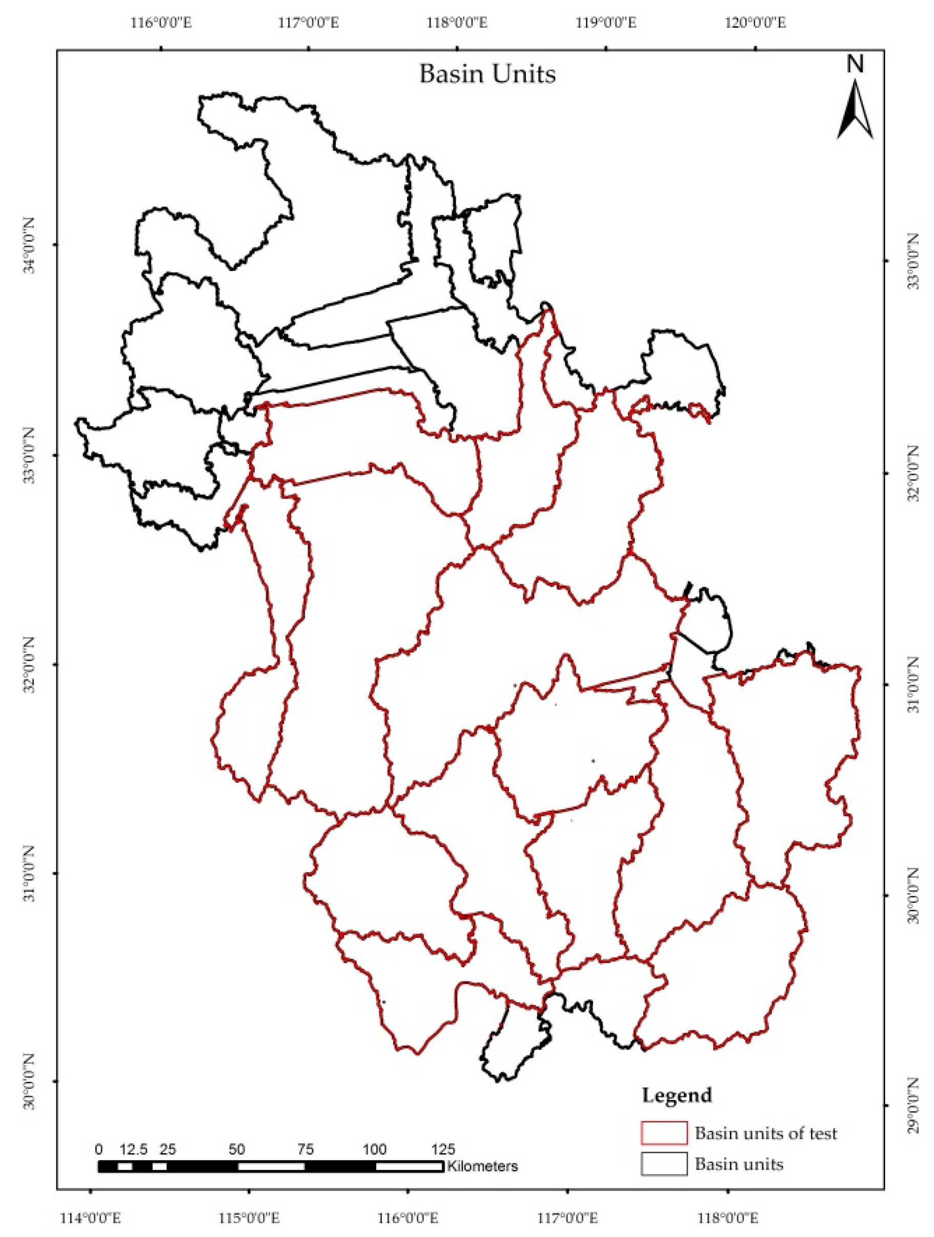
2.1. Study Area
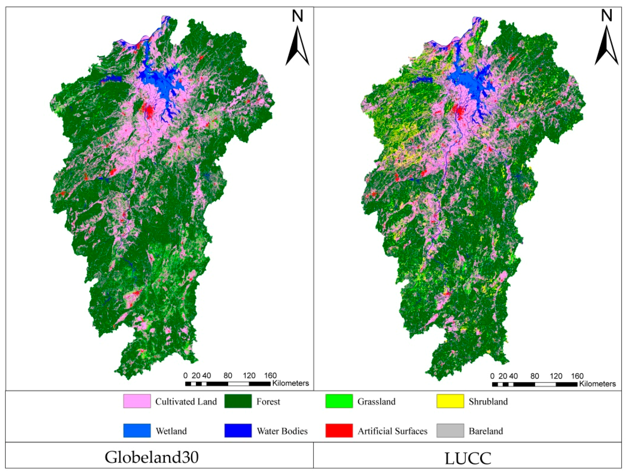
2.2. Data Sources
2.3. Data Processing
2.3.1. Classification System Transformation
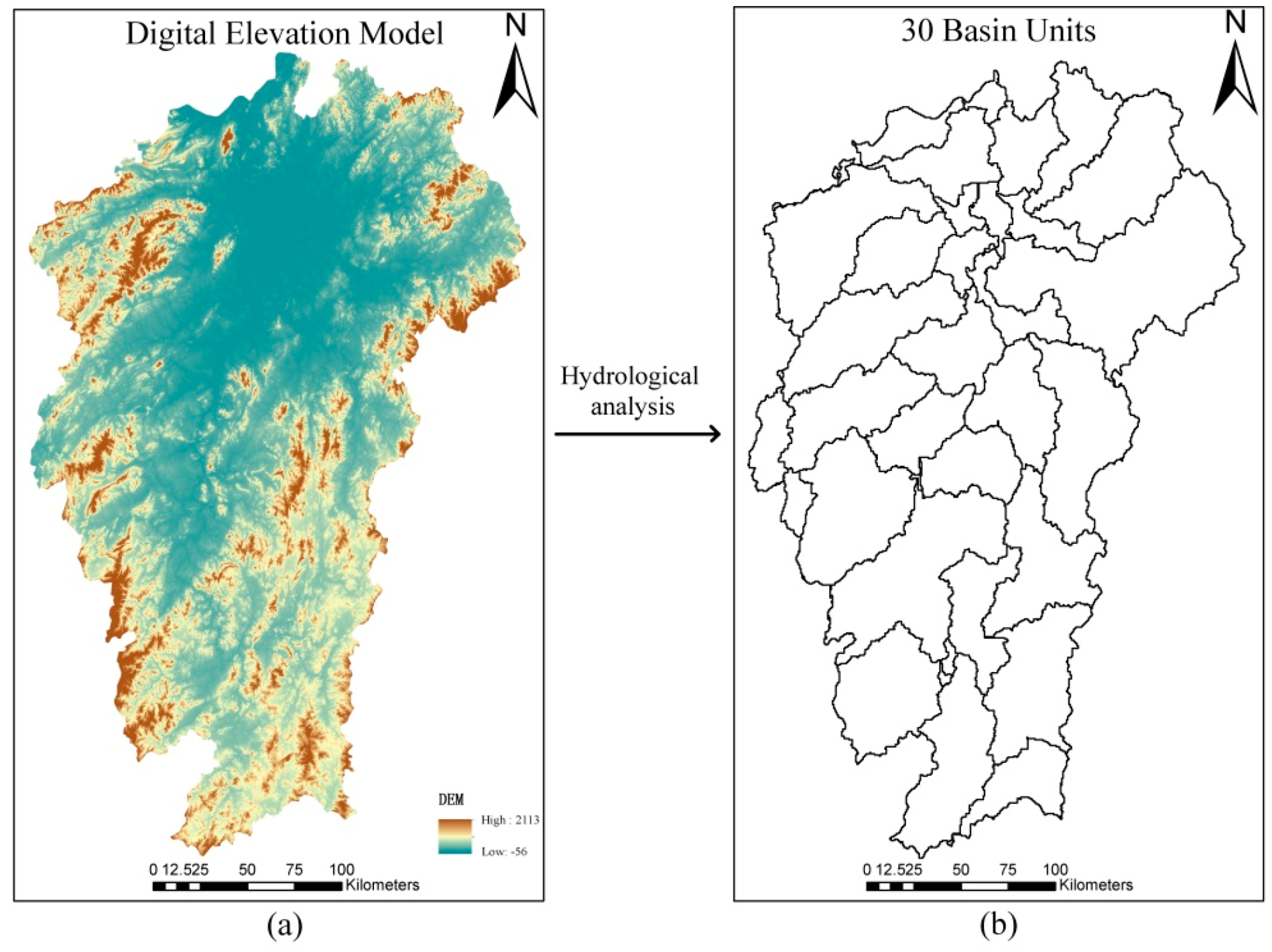
2.3.2. Digital Elevation Model (DEM) Processing
3. Methodology
3.1. Sample Size Determination from Probability Statistical Model
3.2. Determination of Variables in a Multi-Level Linear Model
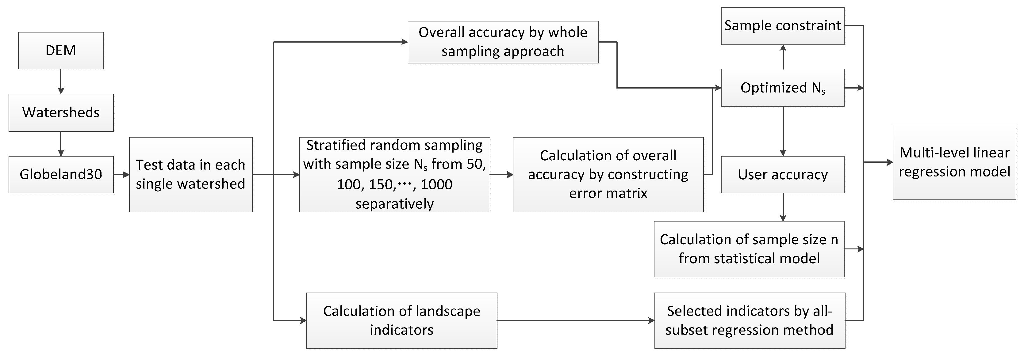
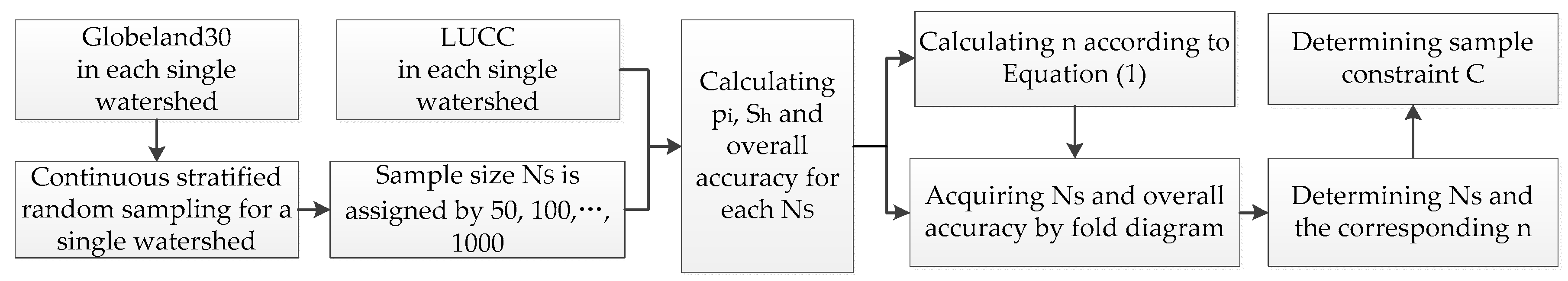
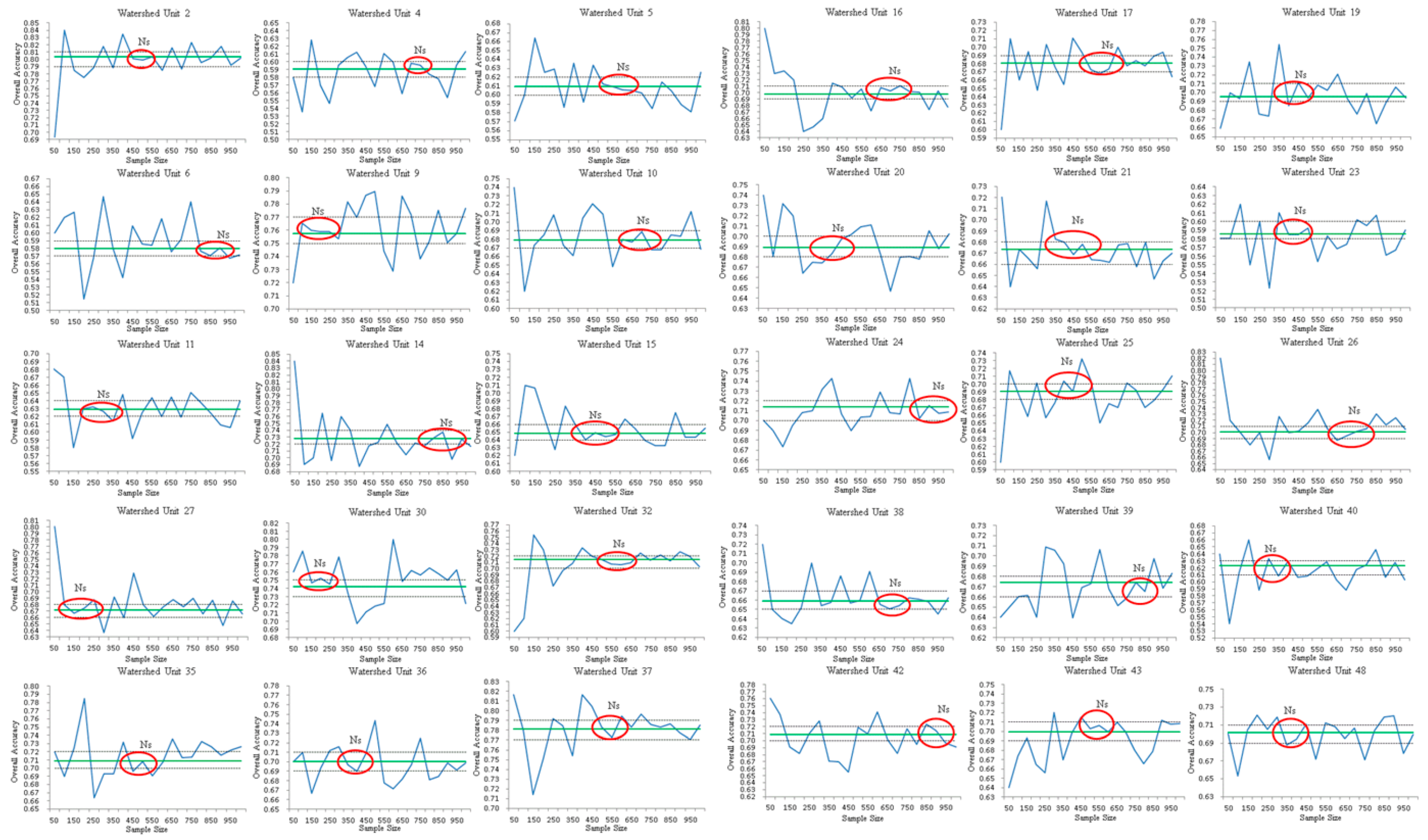
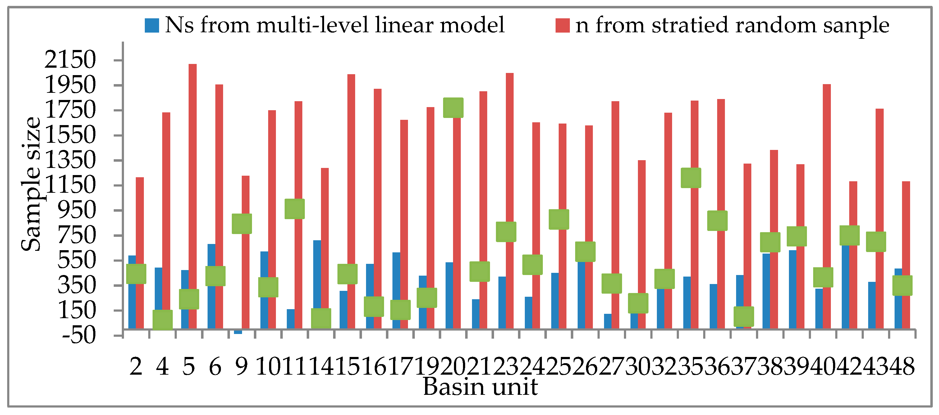
3.2.1. Determining NS, n, and C
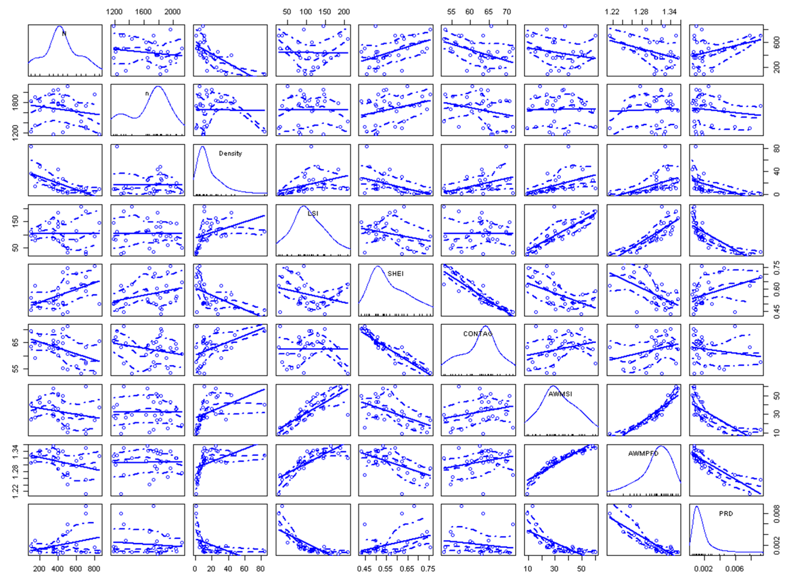
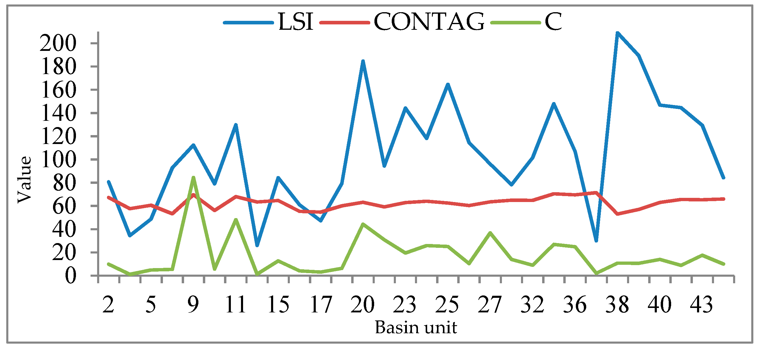
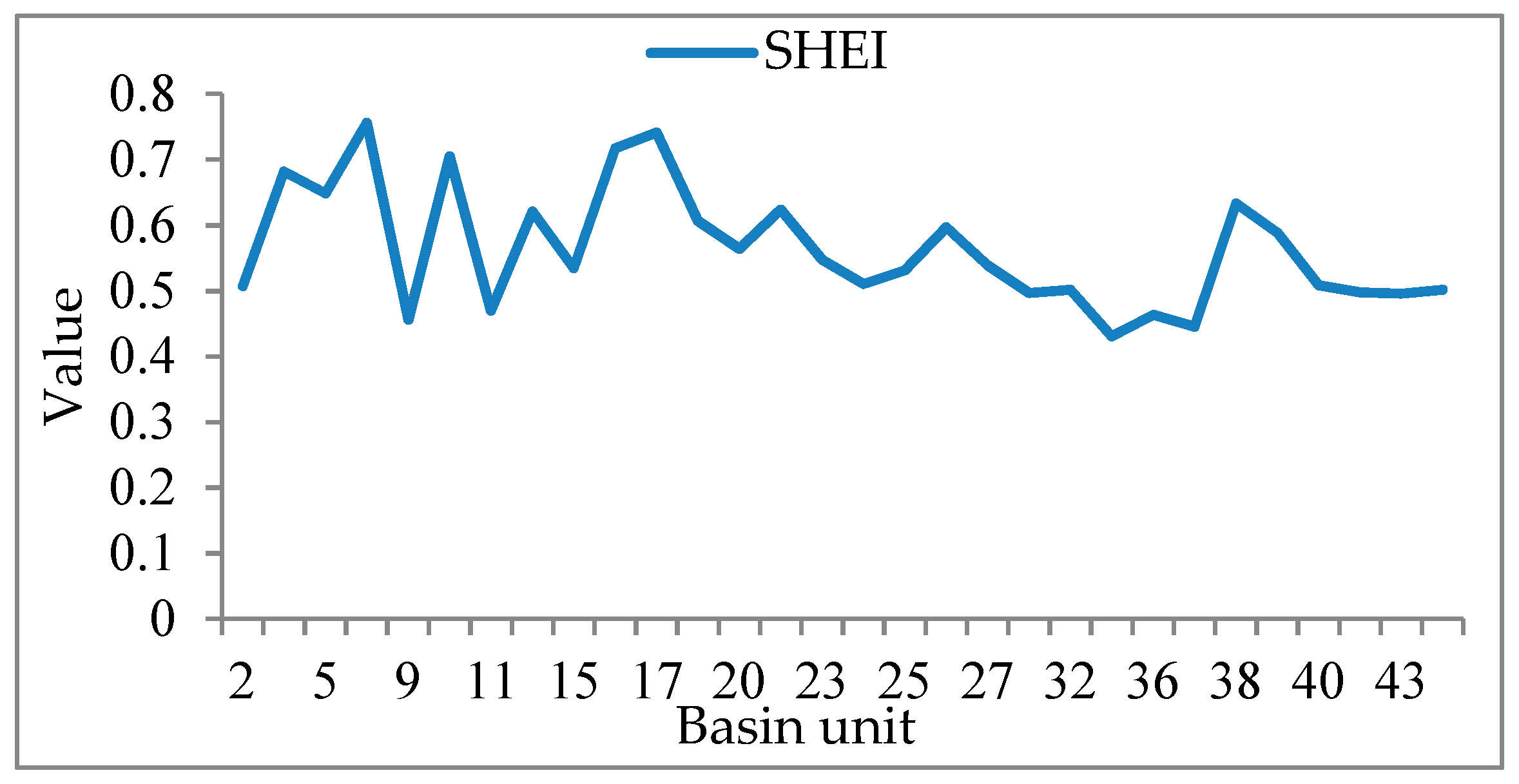
3.2.2. Selection of Landscape Indicators
3.2.3. Regression Analysis
4. Result and Analysis
4.1. Multi-Level Regression
4.2. Model Verification
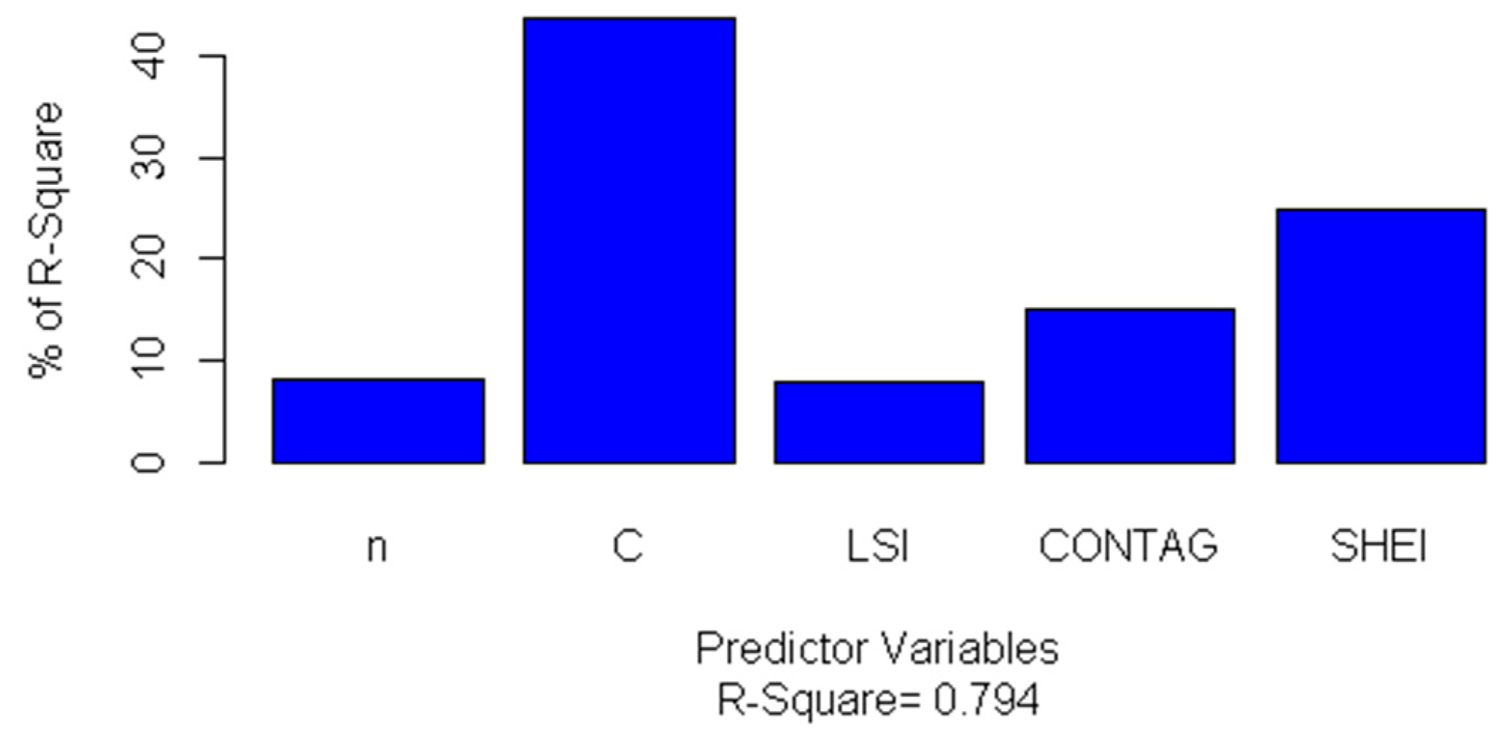
4.3. Relative Importance of Predictor Variables
4.4. Analysis
5. Conclusions
Author Contributions
Funding
Conflicts of Interest
References
- Maria, B.; Monia, M.; Eman, H.; Jun, C.; Ran, L. The First Comprehensive Accuracy Assessment of GlobeLand30 at a National Level: Methodology and Results. Remote Sens. 2015, 7, 4191–4212. [Google Scholar]
- Gallego Pinilla, F.J. Comparing CORINE Land Cover with a more detailed database in Arezzo (Italy). Towards Agric.-Environ. Indic. 2001, 1, 118–125. [Google Scholar]
- Ren, H.; Cai, G.; Zhao, G.; Li, Z. Accuracy assessment of the globeland30 dataset in jiangxi province. ISPRS Int. Arch. Photogramm. Remote Sens. Spat. Inf. Sci. 2018, 3, 1481–1487. [Google Scholar] [CrossRef]
- Chen, J.; Jin, C.; Liao, A.; Xin, C.; Chen, L.; Chen, X.; He, C.; Gang, H.; Shu, P.; Miao, L. Global land cover mapping at 30 m resolution: A POK-based operational approach. ISPRS J. Photogramm. Remote Sens. 2015, 103, 7–27. [Google Scholar] [CrossRef]
- Global Urban Footprint. Available online: http://www.dlr.de/eoc/en/desktopdefault.aspx/tabid-9628/16557_read-40454/ (accessed on 5 August 2018).
- Esch, T.; Heldens, W.; Hirne, A.; Keil, M.; Marconcini, M.; Roth, A.; Zeidler, J.; Dech, S.; Strano, E. Breaking new ground in mapping human settlements from space—The Global Urban Footprint. ISPRS J. Photogramm. Remote Sens. 2017, 134, 30–42. [Google Scholar] [CrossRef]
- Ban, Y.; Gong, P.; Giri, C. Global land cover mapping using Earth observation satellite data: Recent progresses and challenges. ISPRS J. Photogramm. Remote Sens. 2015, 103, 1–6. [Google Scholar] [CrossRef]
- Yang, Y.; Xiao, P.; Feng, X.; Li, H. Accuracy assessment of seven global land cover datasets over China. ISPRS J. Photogramm. Remote Sens. 2017, 125, 156–173. [Google Scholar] [CrossRef]
- Friedl, M.A.; Mciver, D.K.; Hodges, J.C.F.; Zhang, X.Y.; Muchoney, D.; Strahler, A.H.; Woodcock, C.E.; Gopal, S.; Schneider, A.; Cooper, A. Global land cover mapping from MODIS: Algorithms and early results. Remote Sens. Environ. 2002, 83, 287–302. [Google Scholar] [CrossRef]
- Mayaux, P.; Eva, H.; Gallego, J.; Strahler, A.H.; Herold, M.; Agrawal, S.; Naumov, S.; De Miranda, E.E.; Di Bella, C.M.; Ordoyne, C. Validation of the global land cover 2000 map. IEEE Trans. Geosci. Remote Sens. 2006, 44, 1728–1739. [Google Scholar] [CrossRef]
- Tsendbazar, N.E.; Bruin, S.D.; Herold, M. Assessing global land cover reference datasets for different user communities. ISPRS J. Photogramm. Remote Sens. 2014, 103, 93–114. [Google Scholar] [CrossRef]
- Foody, G. Harshness in image classification accuracy assessment. Int. J. Remote Sens. 2008, 29, 3137–3158. [Google Scholar] [CrossRef]
- Herold, M.; Mayaux, P.; Woodcock, C.E.; Baccini, A.; Schmullius, C. Some challenges in global land cover mapping: An assessment of agreement and accuracy in existing 1 km datasets. Remote Sens. Environ. 2008, 112, 2538–2556. [Google Scholar] [CrossRef]
- Curran, P.J.; Williamson, H.D. Sample size for ground and remotely sensed data. Remote Sens. Environ. 1986, 20, 31–41. [Google Scholar] [CrossRef]
- Foody, G.M. Sample size determination for image classification accuracy assessment and comparison. Int. J. Remote Sens. 2009, 30, 5273–5291. [Google Scholar] [CrossRef]
- Martínez-Abraín, A. Are there any differences? A non-sensical question in ecology. Acta Oecol. 2007, 32, 203–206. [Google Scholar] [CrossRef]
- Hay, A.M. Sampling Designs to Test Land-use Map Accuracy. Photogramm. Eng. Remote Sens. 1979, 45, 529–533. [Google Scholar]
- Congalton, R.G. A review of assessing the accuracy of classifications of remotely sensed data. Remote Sens. Environ. 1991, 37, 270–279. [Google Scholar] [CrossRef]
- Liu, H. Sampling Method with Remote Sensing for Monitoring of Cultivated Land Changes on Large Scale. Trans. Chin. Soc. Agric. Eng. 2001, 17, 168–171. [Google Scholar]
- Stehman, S.; Selkowitz, D. A spatially stratified, multi-stage cluster sampling design for assessing accuracy of the Alaska (USA) National Land Cover Database (NLCD). Int. J. Remote Sens. 2010, 31, 1877–1896. [Google Scholar] [CrossRef]
- Ridder, R.M. Options and Recommendations for a Global Remote Sensing Survey of Forests; Forest Resources Assessment Programme Working Paper 141; FAO: Rome, Italy, 2007. [Google Scholar]
- Stehman, S.V.; Olofsson, P.; Woodcock, C.E.; Herold, M.; Friedl, M.A. A global land-cover validation data set, II: Augmenting a stratified sampling design to estimate accuracy by region and land-cover class. Int. J. Remote Sens. 2012, 33, 6975–6993. [Google Scholar] [CrossRef]
- Stehman, S.V. Impact of sample size allocation when using stratified random sampling to estimate accuracy and area of land-cover change. Remote Sens. Lett. 2012, 3, 111–120. [Google Scholar] [CrossRef]
- Fitzpatrick-Lins, K. Comparison of sampling procedures and data analysis for land-use and land-cover map. Photogramm. Eng. Remote Sens. 1981, 47, 343–351. [Google Scholar]
- Congalton, R.G.; Green, K. Assessing the Accuracy of Remotely Sensed Data—Principles and Practice, 2nd ed.; Lewis Publishers: New York, NY, USA, 1999. [Google Scholar]
- Tong, X.; Wang, Z.; Xie, H.; Dan, L.; Jiang, Z.; Li, J.; Li, J. Designing a two-rank acceptance sampling plan for quality inspection of geospatial data products. Comput. Geosci. 2011, 37, 1570–1583. [Google Scholar] [CrossRef]
- Olofsson, P.; Foody, G.M.; Herold, M.; Stehman, S.V.; Woodcock, C.E.; Wulder, M.A. Good practices for estimating area and assessing accuracy of land change. Remote Sens. Environ. 2014, 148, 42–57. [Google Scholar] [CrossRef]
- Stehman, S.V.; Wickham, J.D. Pixels, blocks of pixels, and polygons: Choosing a spatial unit for thematic accuracy assessment. Remote Sens. Environ. 2011, 115, 3044–3055. [Google Scholar] [CrossRef]
- Yin, S.; Chen, X.; Chuanqing, W.U.; Yao, Y.; Wang, X. Spatial-temporal analysis on the variations of the vegetation in Jiangxi Province based on NDVI time series. J. Huazhong Norm. Univ. 2013, 47, 129–135. [Google Scholar]
- Zhao, G.; Cai, G.; Mingyi, D.U. Accuracy Assessment for Land Cover Remote Sensing Mapping Product Based on Landscape Shape Index. Beijing Surv. Mapp. 2017, 1, 271–277. [Google Scholar]
- Chen, J.; Chen, J.; Gong, P.; Liao, A.P.; Chao-Ying, H.E. Higher Resolution Global Land Cover Mapping. Geomat. World 2011, 2, 12–14. [Google Scholar]
- Wang, S.; Liu, J.; Zhang, Z.; Zhou, Q.; Wang, C. Spatial Pattern Change of Land Use in China in Recent 10 Years. Acta Geogr. Sin. 2002, 57, 523–530. [Google Scholar]
- Wang, S.; Liu, J.; Zhang, Z.; Zhou, Q.; Wang, C. Study on spatial pattern and change of land use in recent ten years, China. In Proceedings of the IEEE International Geoscience and Remote Sensing Symposium, Toronto, ON, Canada, 24–28 June 2002; pp. 2369–2371. [Google Scholar]
- Ma, J.; Sun, Q.; Xiao, P.; Wen, B. Accuracy Assessment and Comparative Analysis of GlobeLand30 Dataset in Henan Province. J. Geogr.-Inf. Sci. 2016, 18, 1563–1572. [Google Scholar]
- Huang, Y.; Liao, S. Regional accuracy assessments of the first global land cover dataset at 30-meter resolution: A case study of Henan province. Geogr. Res. 2016, 35, 1433–1446. [Google Scholar]
- Mao, N.; Liu, W.; Wang, H.; Dai, H. Arcgis 10 Tutorial: From Beginner to Master; Surveying and Mapping Publisher: Beijing, China, 2012. [Google Scholar]
- Yi, W.; Yang, P. Determination of drainage area threshold for extraction of DEM-based digital drainage network. Jiangxi Hydraul. Sci. Technol. 2008, 34, 259–262. [Google Scholar]
- Zongmei, L.I.; Zhouqin, M.A.; Nie, Q.; Man, W.; Huang, Y. Method of Ecological Watershed Partitioning. J. China Hydrol. 2017, 37, 27–30. [Google Scholar]
- Stehman, S.V.; Zhang, J.; Foody, G.M. Sampling designs for accuracy assessment of land cover. Int. J. Remote Sens. 2009, 30, 5243–5272. [Google Scholar] [CrossRef]
- Cakir, H.I.; Khorram, S.; Nelson, S.A.C. Correspondence analysis for detecting land cover change. Remote Sens. Environ. 2006, 102, 306–317. [Google Scholar] [CrossRef]
- Olofsson, P.; Kuemmerle, T.; Griffiths, P.; Knorn, J.; Baccini, A.; Gancz, V.; Blujdea, V.; Houghton, R.A.; Abrudan, I.V.; Woodcock, C.E. Carbon implications of forest restitution in post-socialist Romania. Environ. Res. Lett. 2011, 6, 45–202. [Google Scholar] [CrossRef]
- Badjana, H.M.; Olofsson, P.; Woodcock, C.E.; Helmschrot, J.; Wala, K.; Akpagana, K. Mapping and estimating land change between 2001 and 2013 in a heterogeneous landscape in West Africa: Loss of forestlands and capacity building opportunities. Int. J. Appl. Earth Obs. Geoinf. 2017, 63, 15–23. [Google Scholar] [CrossRef]
- Cochran, W.G. Sampling Techniques; John Wiley & Sons.: New York, NY, USA, 1977. [Google Scholar]
- Olofsson, P.; Foody, G.M.; Stehman, S.V.; Woodcock, C.E. Making better use of accuracy data in land change studies: Estimating accuracy and area and quantifying uncertainty using stratified estimation. Remote Sens. Environ. 2013, 129, 122–131. [Google Scholar] [CrossRef]
- Chen, J.; Chen, J.; Hao, W.; Hou, D.Y.; Zhang, W.W.; Zhang, J.; Zhou, X.G.; Chen, L.J. A landscape shape index-based sampling approach for land cover accuracy assessment. Sci. China Earth Sci. 2016, 59, 1–12. [Google Scholar] [CrossRef]
- Crews-Meyer, K.; Hudson, P.; Colditz, R.R. Landscape Complexity and Remote Classification in Eastern Coastal Mexico: Applications of Landsatâ-7 ETM+ Data. Geocarto Int. 2004, 19, 45–56. [Google Scholar] [CrossRef]
- Neel, M.C.; Mcgarigal, K.; Cushman, S.A. Behavior of class-level landscape metrics across gradients of class aggregation and area. Landsc. Ecol. 2003, 19, 435–455. [Google Scholar] [CrossRef]
- Huang, D.; Ke, C.; Wang, Z.; Shuang, L.; Information, S.O.; University, S.O. Accuracy assessment method for remote sensing image classification results based on spatial sampling theory. Comput. Appl. Softw. 2016, 33, 190–194. [Google Scholar]
- Sun, W.; Du, B.; Xiong, S. Quantifying Sub-Pixel Surface Water Coverage in Urban Environments Using Low-Albedo Fraction from Landsat Imagery. Remote Sens. 2017, 9, 428. [Google Scholar] [CrossRef]
- Sun, W.; Halevy, A.; Benedetto, J.J.; Czaja, W.; Li, W.; Liu, C.; Shi, B.; Wang, R. Nonlinear Dimensionality Reduction via the ENH-LTSA Method for Hyperspectral Image Classification. IEEE J. Sel. Top. Appl. Earth Obs. Remote Sens. 2014, 7, 375–388. [Google Scholar] [CrossRef]
- Cai, G.; Du, M.; Gao, Y. City block-based assessment of land cover components’ impacts on the urban thermal environment. Remote Sens. Appl. Soc. Environ. 2019, 13, 85–96. [Google Scholar] [CrossRef]
- Kabacoff, R. R in Action: Data Analysis and Graphics with R, 2nd ed.; Manning Publications: Shelter Island, NY, USA, 2011. [Google Scholar]
- Kohavi, R. A Study of Cross-Validation and Bootstrap for Accuracy Estimation and Model Selection. Int. Jt Conf. Artif. Intell. 1995, 2, 1137–1143. [Google Scholar]
- Johnson, J.W. Factors Affecting Relative Weights: The Influence of Sampling and Measurement Error. Organ. Res. Methods 2004, 7, 283–299. [Google Scholar] [CrossRef]


| Globeland30 | Land Use/Cover Change (LUCC) | ||
|---|---|---|---|
| Index | Class Name | Index | Class Name |
| 10 | Cultivated Land | 11 | Paddy Land |
| 12 | Dry Land | ||
| 20 | Forest | 21 | Forest |
| 23 | Woods | ||
| 24 | Others | ||
| 30 | Grassland | 31 | Dense Grass |
| 32 | Moderate Grass | ||
| 33 | Sparse Grass | ||
| 40 | Shrubland | 22 | Shrub |
| 50 | Wetland | 46 | Bottom Land |
| 64 | Swampland | ||
| 60 | Water Bodies | 41 | Stream and Rivers |
| 42 | Lakes | ||
| 43 | Reservoir and Ponds | ||
| 80 | Artificial Surfaces | 51 | Urban Built-up |
| 52 | Rural Settlements | ||
| 53 | Others | ||
| 90 | Bare Land | 65 | Bare soil |
| 67 | Others | ||
| Wh | NS | ||||||||||||||||||||
|---|---|---|---|---|---|---|---|---|---|---|---|---|---|---|---|---|---|---|---|---|---|
| 50 | 100 | 150 | 200 | 250 | 300 | 350 | 400 | 450 | 500 | 550 | 600 | 650 | 700 | 750 | 800 | 850 | 900 | 950 | 1000 | ||
| S1 | 0.23 | 0.47 | 0.41 | 0.42 | 0.49 | 0.49 | 0.41 | 0.45 | 0.41 | 0.39 | 0.46 | 0.45 | 0.47 | 0.43 | 0.44 | 0.39 | 0.46 | 0.47 | 0.40 | 0.45 | 0.44 |
| S2 | 0.67 | 0.41 | 0.29 | 0.32 | 0.33 | 0.25 | 0.28 | 0.34 | 0.30 | 0.35 | 0.31 | 0.29 | 0.32 | 0.30 | 0.34 | 0.32 | 0.32 | 0.31 | 0.29 | 0.31 | 0.33 |
| S3 | 0.05 | - | 0.00 | 0.33 | 0.33 | 0.27 | 0.00 | 0.00 | 0.25 | 0.00 | 0.35 | 0.28 | 0.20 | 0.26 | 0.40 | 0.29 | 0.35 | 0.31 | 0.22 | 0.33 | 0.25 |
| S4 | 0.00 | - | - | - | - | - | - | - | - | - | - | - | - | - | - | - | - | - | - | - | - |
| S5 | 0.02 | 0.47 | 0.50 | 0.47 | 0.49 | 0.00 | 0.35 | 0.50 | 0.33 | 0.33 | 0.40 | 0.49 | 0.50 | 0.48 | 0.43 | 0.49 | 0.48 | 0.46 | 0.48 | 0.49 | 0.43 |
| S6 | 0.02 | - | 0.00 | 0.47 | 0.50 | 0.35 | 0.50 | 0.50 | 0.45 | 0.47 | 0.46 | 0.50 | 0.49 | 0.48 | 0.50 | 0.39 | 0.50 | 0.45 | 0.50 | 0.50 | 0.47 |
| S7 | 0.02 | 0.00 | 0.00 | 0.49 | 0.47 | 0.50 | 0.49 | 0.50 | 0.47 | 0.48 | 0.49 | 0.49 | 0.47 | 0.49 | 0.48 | 0.50 | 0.36 | 0.39 | 0.45 | 0.46 | 0.43 |
| S8 | 0.00 | - | - | - | - | - | - | - | - | - | 0.00 | - | 0.00 | - | 0.00 | - | 0.00 | - | - | 0.00 | - |
| Class | Name | Unit | Range |
|---|---|---|---|
| Area Metrics | Largest Patch Index (LPI) | % | (0,1) |
| Contrast Metrics | Mean Patch Size (MPS) | hm2 | >0 |
| Edge Metrics | Edge Density (ED) | m/hm2 | -- |
| Patch density (PD) | -- | >0 | |
| Shape Metrics | Landscape shape index (LSI) | -- | ≥1 |
| Area-weighted mean shape index (AWMSI) | -- | (1,2) | |
| Area-weighted Mean patch fractal dimension (AWMPFD) | -- | [1,2] | |
| Proximity Metrics | Mean proximity index (MPI) | -- | >0 |
| Diversity Metrics | Shannon’s diversity index (SHDI) | -- | ≥0 |
| Patch richness density (PRD) | -- | >0 | |
| Shannon’s evenness index (SHEI) | -- | (0,1) | |
| Aggregation Metrics | Interspersion and Juxtaposition index (IJI) | % | (0,100) |
| Contagion index (CONTAG) | % | (0,100) |
| Estimate | Standard Error | t Value | Pr (>|t|) | Significance Codes | |
|---|---|---|---|---|---|
| (Intercept) | −17,880 | 5846 | −3.058 | 5.97 × 10⁻³ | 0.01 |
| n | −0.278 | 0.076 | −3.658 | 1.47 × 10⁻³ | 0.01 |
| C | −9.392 | 1.344 | −6.987 | 6.72 × 10⁻⁷ | 0.001 |
| LSI | 5.479 | 1.026 | 5.34 | 2.70 × 10⁻⁵ | 0.001 |
| CONTAG | 109.900 | 23.380 | 4.699 | 1.22 × 10⁻⁴ | 0.001 |
| SHEI | 7163 | 1465 | 4.89 | 7.78 × 10⁻⁵ | 0.001 |
| AWMSI | −7.424 | 4.932 | −1.505 | 1.47 × 10⁻¹ | 1 |
| AWMPFD | 5803 | 3092 | 1.877 | 7.45 × 10⁻² | 0.1 |
| PRD | 48,490 | 20,160 | 2.405 | 2.55 × 10⁻² | 0.05 |
| Residual standard error | 95.28 on 21 degrees of freedom | ||||
| Multiple R2 squared | 0.8384 | ||||
| Adjusted R2 squared | 0.7768 | ||||
| F-statistic | 13.62 on 8 and 21 DF | ||||
| p-value | <9.80 × 10⁻⁷ | ||||
| Estimate | Standard Error | t Value | Pr(>|t|) | Significance Codes | |
|---|---|---|---|---|---|
| (Intercept) | −7159 | 1632 | −4.386 | 1.98 × 10⁻⁴ | 0.001 |
| n | −0.255 | 0.070 | −3.627 | 1.34 × 10⁻³ | 0.01 |
| C | −9.261 | 1.366 | −6.781 | 5.16 × 10⁻⁷ | 0.001 |
| LSI | 4.210 | 0.762 | 5.523 | 1.11 × 10⁻⁵ | 0.001 |
| CONTAG | 77.900 | 16.960 | 4.592 | 1.17 × 10⁻⁴ | 0.001 |
| SHEI | 5085 | 960.500 | 5.294 | 1.98 × 10⁻⁵ | 0.001 |
| Residual standard error | 100.7 on 24 degrees of freedom | ||||
| Multiple R2 squared | 0.7935 | ||||
| Adjusted R2 squared | 0.7505 | ||||
| F-statistic | 18.45 on 5 and 24 DF | ||||
| p-value | 1.58 × 10⁻⁷ | ||||
| Original R-square | 0.7935414 |
| Three-fold cross-validated R-square | 0.634445 |
| Change | 0.1590964 |
| Method | Multi-LEVEL Model | Statistical Model | Absolute Value of OA Difference (%) | Sample Size Difference (NS-n) | |||
|---|---|---|---|---|---|---|---|
| Units Code | NS | OA (%) | n | OA (%) | |||
| No.1_Ah | 475 | 79.62 | 1511 | 79.56 | 0.06 | 1035 | |
| No.2_Ah | 675 | 79.56 | 1388 | 79.54 | 0.02 | 714 | |
| No.3_Ah | 1288 | 56.06 | 1561 | 56.63 | 0.57 | 274 | |
| No.4_Ah | 1110 | 68.38 | 1620 | 68.40 | 0.02 | 510 | |
| No.5_Ah | 485 | 77.11 | 1759 | 77.37 | 0.26 | 1274 | |
| No.6_Ah | 956 | 75.10 | 1556 | 76.56 | 1.45 | 601 | |
| No.7_Ah | 922 | 73.64 | 1591 | 69.94 | 3.71 | 669 | |
| No.8_Ah | 879 | 66.78 | 2045 | 67.63 | 0.85 | 1166 | |
| No.9_Ah | 978 | 69.19 | 1979 | 67.66 | 1.53 | 1002 | |
| No.10_Ah | 1106 | 59.19 | 1902 | 59.94 | 0.75 | 796 | |
| No.11_Ah | 696 | 52.65 | 2186 | 48.86 | 3.80 | 1490 | |
| No.12_Ah | 1128 | 64.69 | 1384 | 66.16 | 1.47 | 256 | |
| No.13_Ah | 912 | 61.95 | 2006 | 63.24 | 1.29 | 1093 | |
| No.14_Ah | 790 | 63.29 | 1935 | 64.50 | 1.20 | 1145 | |
| Sum = 12,399 | Sum= 24,425 | Average = 1.21 | Sum = 12,026 | ||||
| Independent Variable | n | C | LSI | CONTAG | SHEI |
|---|---|---|---|---|---|
| Standardised regression coefficients | −3.60 × 10⁻¹ | −8.13 × 10⁻¹ | 9.90 × 10⁻¹ | 1.97 | 2.31 |
| Relative importance level | 5 | 4 | 3 | 2 | 1 |
© 2019 by the authors. Licensee MDPI, Basel, Switzerland. This article is an open access article distributed under the terms and conditions of the Creative Commons Attribution (CC BY) license (http://creativecommons.org/licenses/by/4.0/).
Share and Cite
Ren, H.; Cai, G.; Du, M. Surface Heterogeneity-Involved Estimation of Sample Size for Accuracy Assessment of Land Cover Product from Satellite Imagery. Sensors 2019, 19, 4430. https://doi.org/10.3390/s19204430
Ren H, Cai G, Du M. Surface Heterogeneity-Involved Estimation of Sample Size for Accuracy Assessment of Land Cover Product from Satellite Imagery. Sensors. 2019; 19(20):4430. https://doi.org/10.3390/s19204430
Chicago/Turabian StyleRen, Huiqun, Guoyin Cai, and Mingyi Du. 2019. "Surface Heterogeneity-Involved Estimation of Sample Size for Accuracy Assessment of Land Cover Product from Satellite Imagery" Sensors 19, no. 20: 4430. https://doi.org/10.3390/s19204430
APA StyleRen, H., Cai, G., & Du, M. (2019). Surface Heterogeneity-Involved Estimation of Sample Size for Accuracy Assessment of Land Cover Product from Satellite Imagery. Sensors, 19(20), 4430. https://doi.org/10.3390/s19204430