Blind Fractionally Spaced Channel Equalization for Shallow Water PPM Digital Communications Links


Abstract
1. Introduction
1.1. Potential Limits of OFDM
1.2. Merits of Single-Carrier Schemes
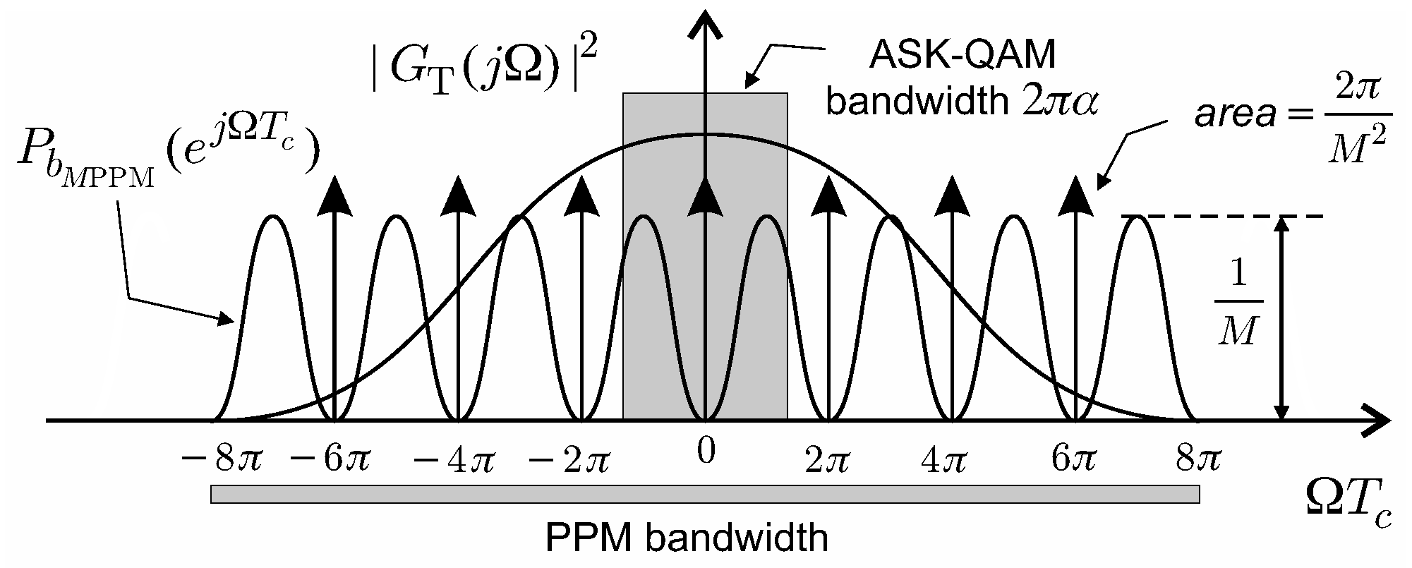
2. MPPM Waveform
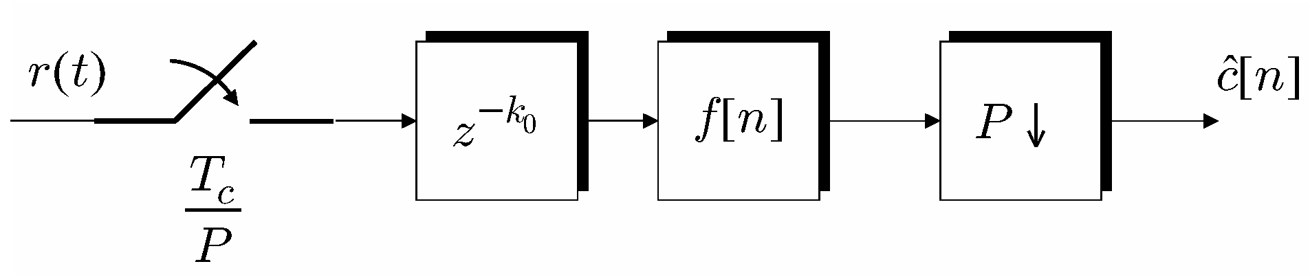
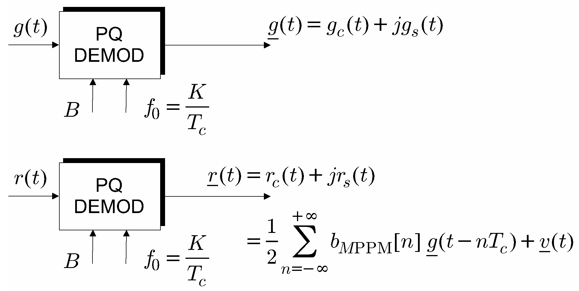
3. MPPM Receiver
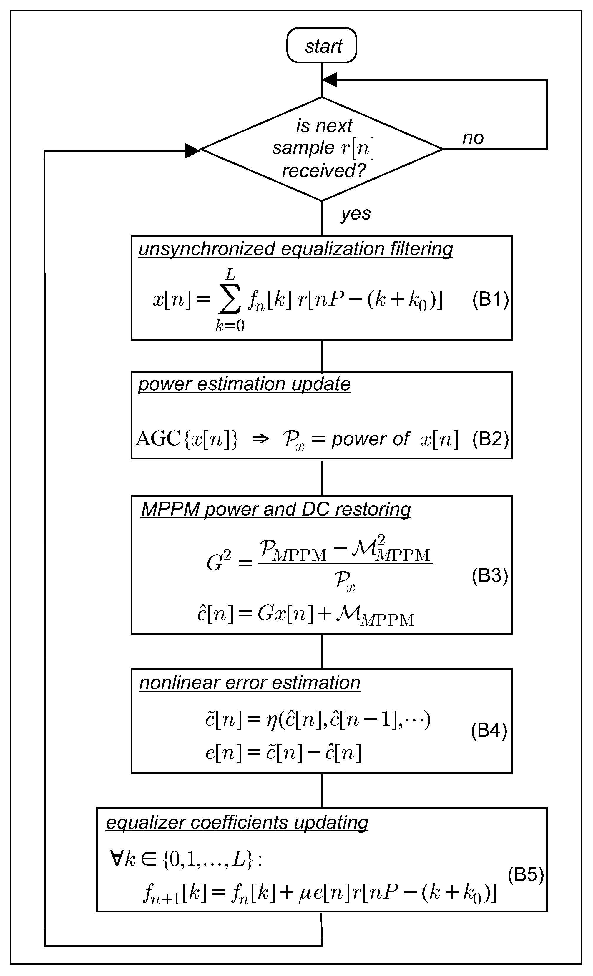
4. Trained and Blind Fractionally Spaced Equalization
- The development of the MMSE nonlinearity that fully exploits the probabilistic description of the MPPM symbol formed as in (1);
- The proof of how the probabilistic description of the MPPM symbol (1) can be employed to recover the symbol timing;
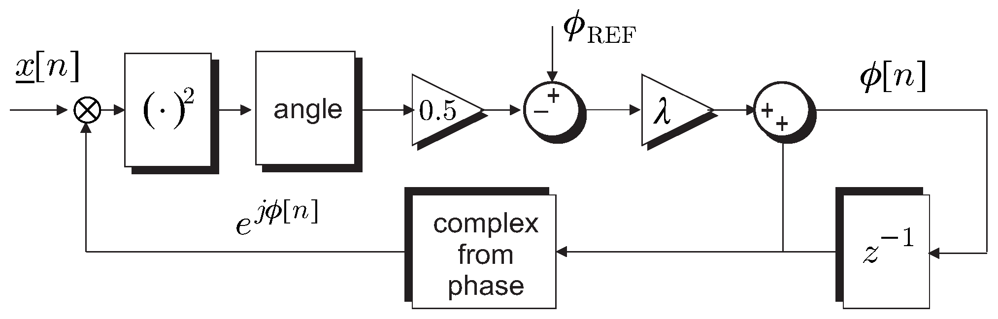
- The introduction of a blind channel phase recovery technique that exploits the redundancy present in band-pass MPPM signals; it is worth highlighting that such a phase recovery stage is mandatory for band-pass transmission and coherent detection, and it is a critical step even in data aided (trained) equalization.
4.1. LMS Trained FSE
4.2. LMS Blind Bussgang FSE
- A1.
- A2.
- The output of the FSE is assumed to satisfy the following additive white gaussian noise (AWGN) signal model:being a realization of stationary white Gaussian random series of power and statistically independent of .
- Sync: collects all the binary M-tuples that have zero valued elements, i.e., the M rows of the identity M-matrix , so that its cardinality is M;
- Unsync: joins with the binary M-tuple that has all zeros as well as with all the binary M-tuples that have zeros; since these latter occurs in number of , it results:
5. Numerical Results
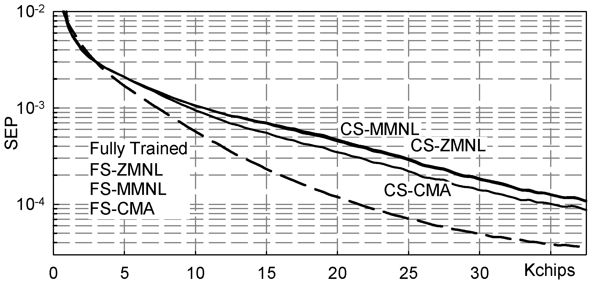
5.1. Severe Three-Paths Channel
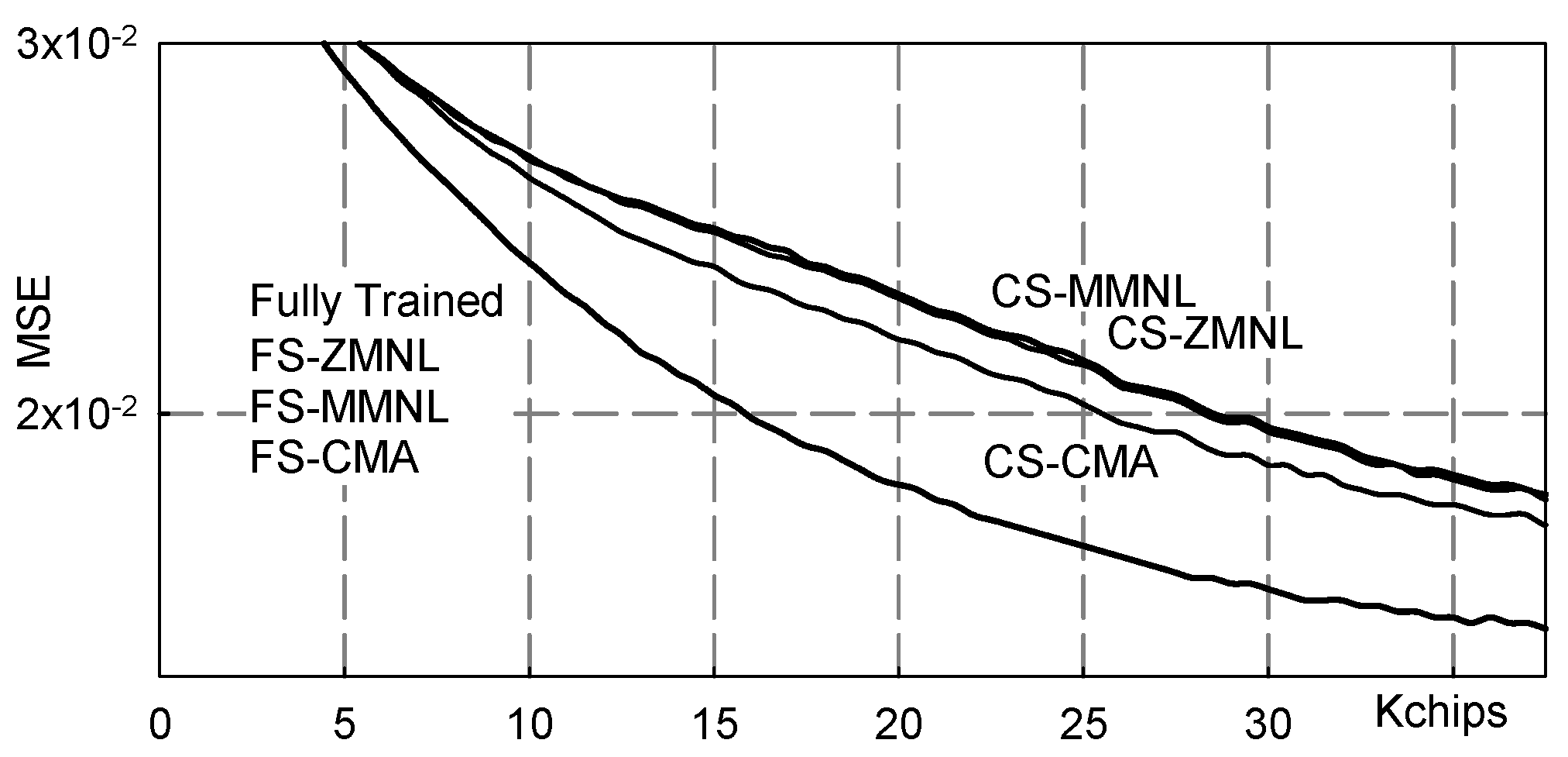
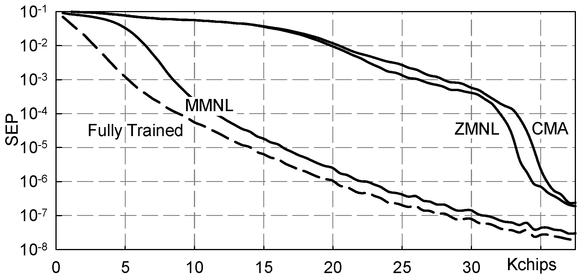
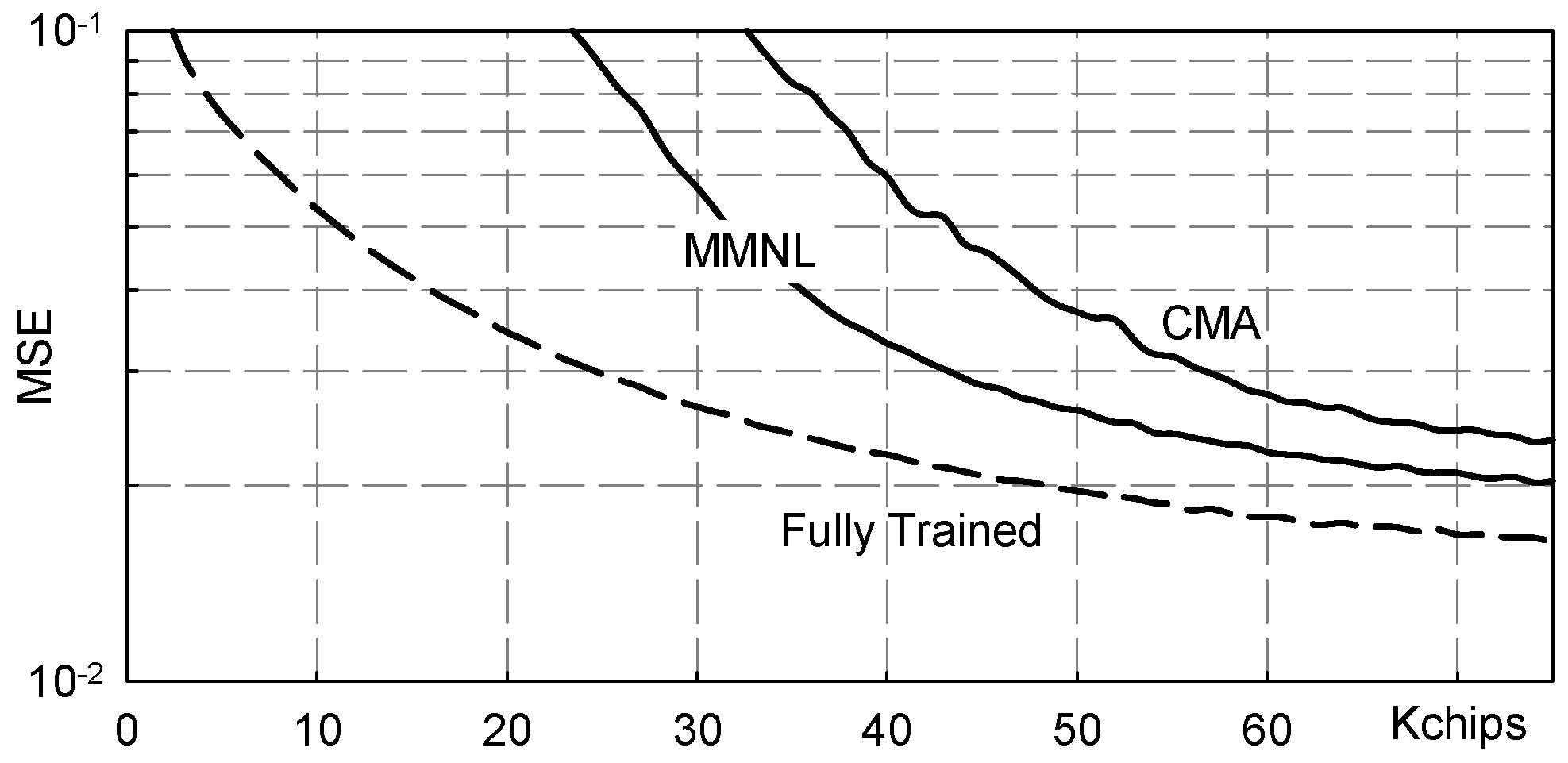
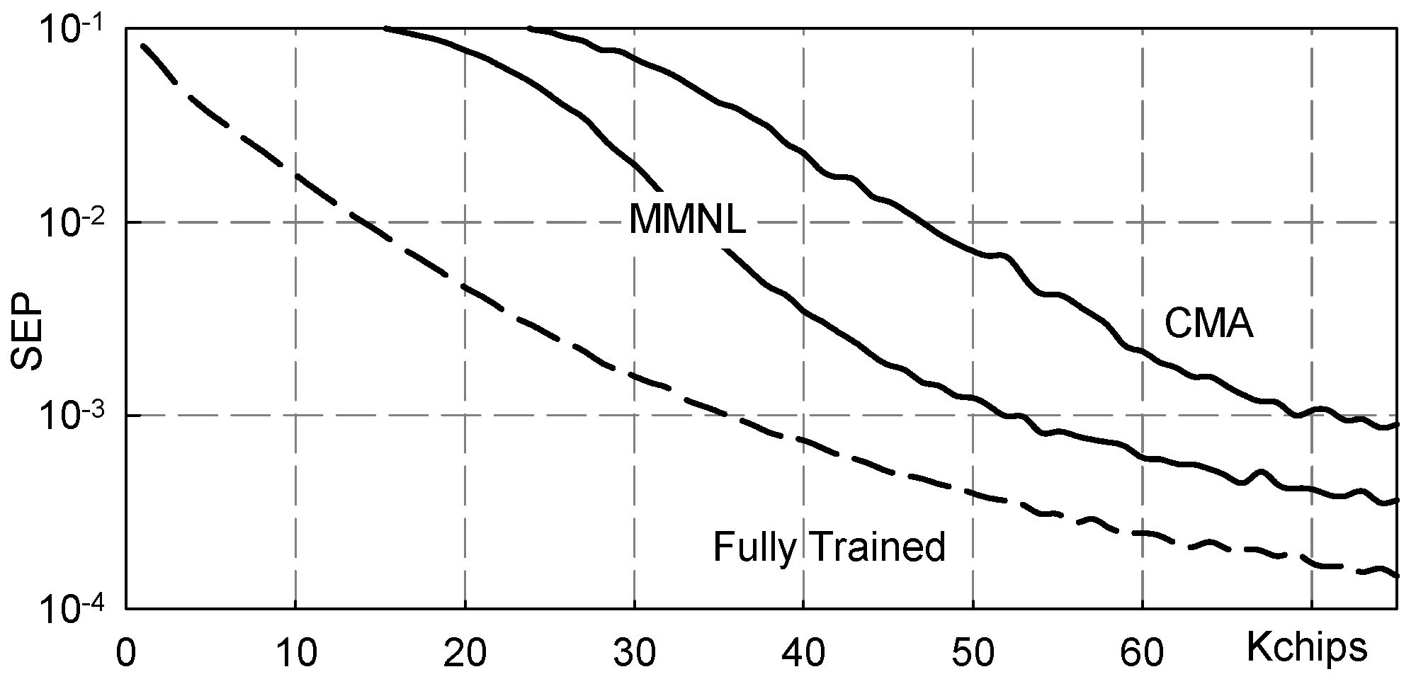
- Fully Trained: the ideal data-aided fractionally spaced equalizer that knows all the transmitted symbols;
- FS-MMNL: the blind fractionally spaced Bussgang equalizer that uses the novel M-memory nonlinearity (B4) here presented;
- FS-ZMNL: the blind fractionally spaced Bussgang equalizer that uses the zero-memory nonlinearity described in [23];
- FS-CMA: the blind fractionally spaced CMA equalizer [28];
- CS-MMNL: the blind chip spaced Bussgang equalizer that uses the novel M-memory nonlinearity (B4);
- CS-ZMNL: the blind chip spaced Bussgang equalizer that uses the zero-memory nonlinearity described in [23];
- CS-CMA: the blind chip spaced CMA equalizer [28].
5.2. Multipath Channel
5.3. Severe Multipath Channel
6. Conclusions
Author Contributions
Funding
Conflicts of Interest
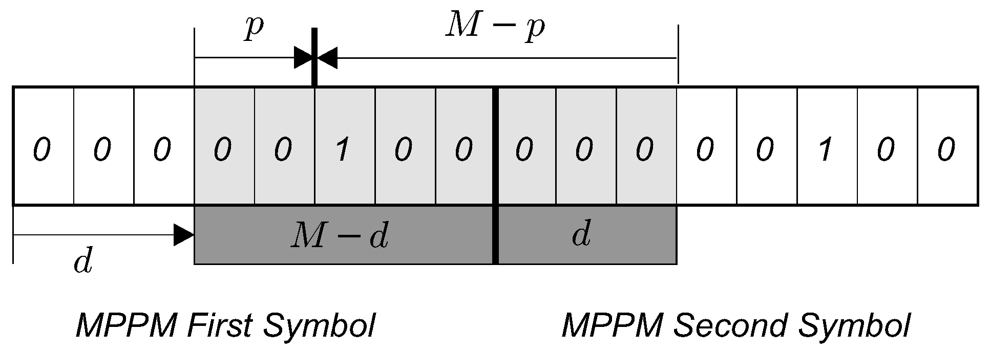
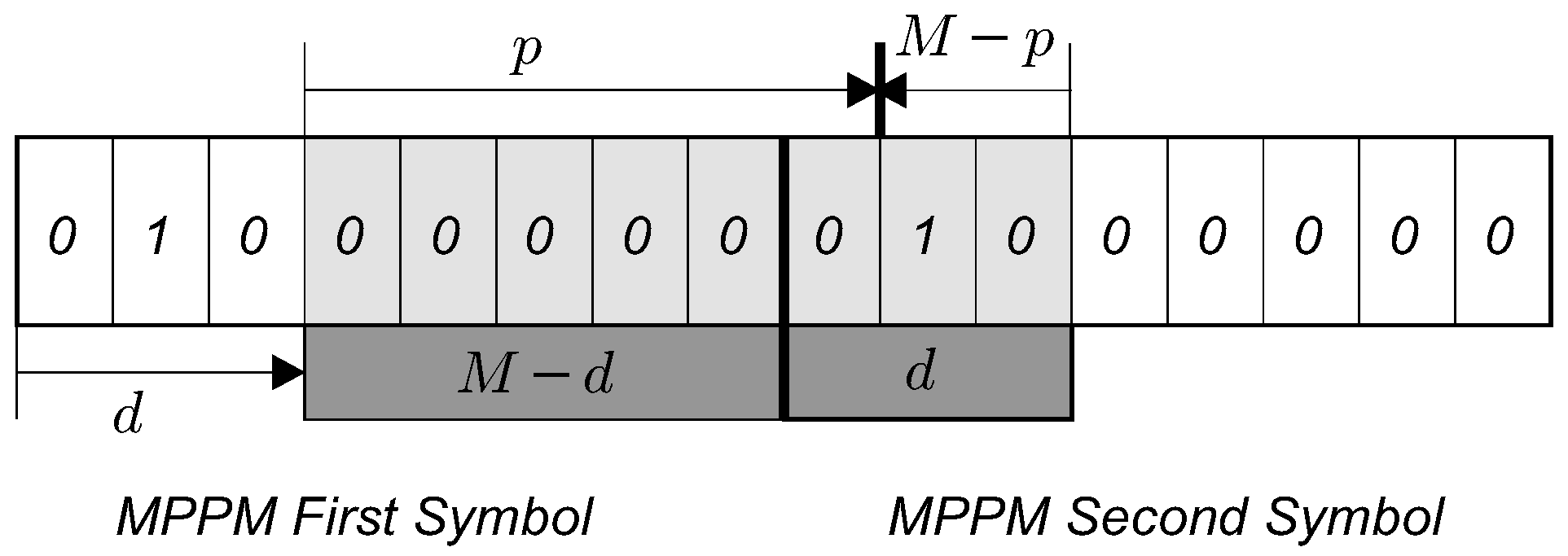
Appendix A. Binary M-Tuple Probabilities Evaluation
Appendix A.1. Case 1: Single Chip 1 at Position p


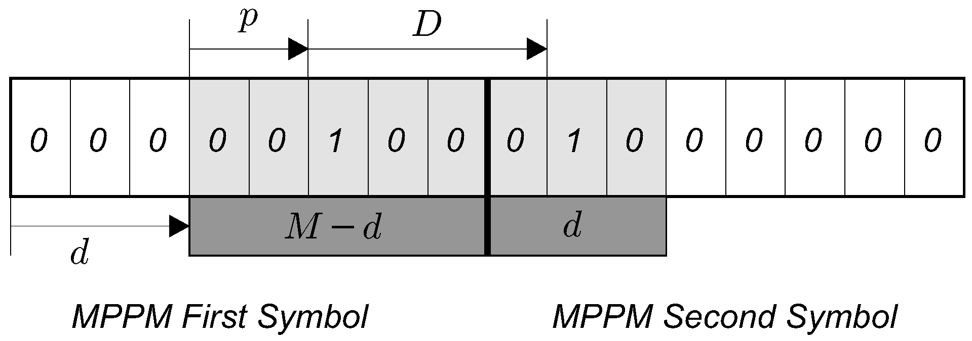
Appendix A.2. Case 2: Two Chips 1 Distant D Positions

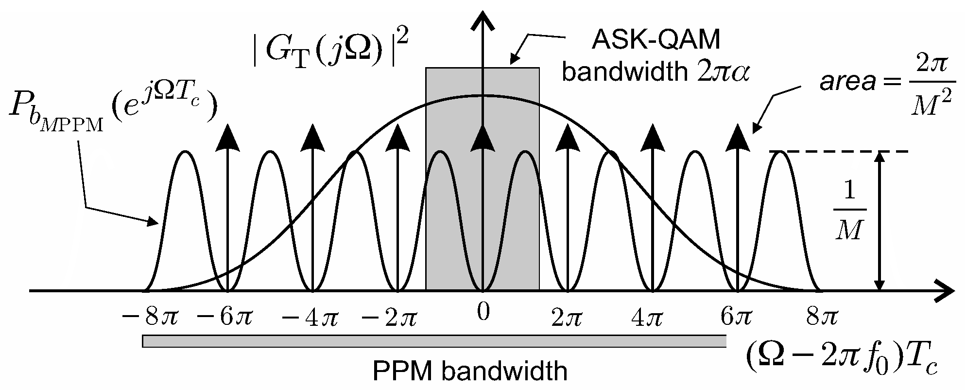
Appendix B. Complex Low-Pass Representation of Band-Pass MPPM Signals


Appendix Automatic Phase Controls


References
- Stojanovic, M.; Preisig, J. Underwater acoustic communication channels: Propagation models and statistical characterization. IEEE Commun. Mag. 2009, 47, 84–89. [Google Scholar] [CrossRef]
- Proakis, J.G. Adaptive equalization techniques for acoustic telemetry channels. IEEE J. Ocean. Eng. 1991, 16, 21–31. [Google Scholar] [CrossRef]
- Zhao, S.; Zhang, X.; Zhang, X. Iterative frequency domain equalization combined with LDPC decoding for single-carrier underwater acoustic communications. In Proceedings of the OCEANS 2016 MTS/IEEE Monterey, Monterey, CA, USA, 19–23 September 2016; pp. 1–5. [Google Scholar]
- Liu, L.; Zhang, Y.; Zhang, P.; Zhou, L.; Niu, J. Channel coding for underwater acoustic single-carrier CDMA communication system. In Proceedings of the 7th International Conference on Electronics and Information Engineering, Nanjing, China, 23 January 2017; pp. 671–680. [Google Scholar]
- Chithra, K.; Sireesha, N.; Thangavel, C.; Gowthaman, V.; Narayanan, S.S.; Sudhakar, T.; Atmanand, M.A. Underwater communication implementation with OFDM. Indian J. Geo-Mar. Sci. 2015, 44, 259–266. [Google Scholar]
- Hessien, S.; Tokgöz, S.C.; Anous, N.; Boyacı, A.; Abdallah, M.; Qaraqe, K.A. Experimental evaluation of OFDM-based underwater visible light communication cystem. IEEE Photonics J. 2018, 10, 1–13. [Google Scholar] [CrossRef]
- Ashri, R.; Shaban, H.; El-Nasr, M. A novel fractional Fourier transform-based ASK-OFDM system for underwater acoustic communications. Appl. Sci. 2017, 7, 1286. [Google Scholar] [CrossRef]
- Liu, S.; Ma, T.; Qiao, G.; Ma, L.; Yin, Y. Biologically inspired covert underwater acoustic communication by mimicking dolphin whistles. Appl. Acoust. 2017, 120, 120–128. [Google Scholar] [CrossRef]
- Li, B.; Huang, J.; Zhou, S.; Ball, K.; Stojanovic, M.; Freitag, L.; Willett, P. MIMO-OFDM for high-rate underwater acoustic communications. IEEE J. Ocean. Eng. 2009, 34, 634–644. [Google Scholar]
- Stojanovic, M. OFDM for underwater acoustic communications: Adaptive synchronization and sparse channel estimation. In Proceedings of the 2008 IEEE International Conference on Acoustics, Speech and Signal Processing, Las Vegas, NV, USA, 31 March–4 April 2008; pp. 5288–5291. [Google Scholar]
- Klein, A.G.; Johnson, C.R. MMSE decision feedback equalization of pulse position modulated signals. In Proceedings of the EEE International Conference on Communications, Paris, France, 20–24 June 2004; Volume 5, pp. 2648–2652. [Google Scholar]
- Ungerboeck, G. Fractional tap-spacing equalizer and consequences for clock recovery in data modems. IEEE Trans. Commun. 1976, 24, 856–864. [Google Scholar] [CrossRef]
- Scarano, G.; Petroni, A.; Biagi, M.; Cusani, R. Second-order statistics driven LMS blind fractionally spaced channel equalization. IEEE Signal Process. Lett. 2017, 24, 161–165. [Google Scholar] [CrossRef]
- Xiao, Y. Recursive least squares fractionally-spaced blind equalization algorithm for underwater acoustic communication. J. Inf. Comput. Sci. 2013, 10, 6077–6084. [Google Scholar] [CrossRef][Green Version]
- Artman, D.J.; Chari, S.; Gooch, R.P. Joint equalization and timing recovery in a fractionally-spaced equalizer. In Proceedings of the 1992 Conference Record of the Twenty-Sixth Asilomar Conference on Signals, Systems and Computers, Pacific Grove, CA, USA, 26–28 October 1992; Volume 1, pp. 25–29. [Google Scholar]
- Nasir, A.A.; Durrani, S.; Kennedy, R.A. Blind fractionally spaced equalization and timing synchronization in wireless fading channels. In Proceedings of the 2010 2nd International Conference on Future Computer and Communication, Wuha, China, 21–24 May 2010; Volume 3, pp. 15–19. [Google Scholar]
- Scarano, G.; Petroni, A.; Cusani, R.; Biagi, M. Sampling phase estimation in underwater PPM fractionally sampled equalization. In Proceedings of the 26th European Signal Processing Conference (EUSIPCO), Rome, Italy, 3–7 September 2018; pp. 912–916. [Google Scholar]
- Biglieri, E.; Benedetto, S. Principles of Digital Transmission; Kluwer Academic Publisher: New York, NY, USA, 1999. [Google Scholar]
- Scarano, G. Lezioni di Elaborazione Statistica dei Segnali (Vol.II). Available online: https://www.amazon.it/Elaborazione-Statistica-dei-Segnali-vol-II/dp/1549794752 (accessed on 22 September 2017).
- Godfrey, R.; Rocca, F. Zero memory non-linear deconvolution. Geophys. Pros. 1981, 29, 189–228. [Google Scholar] [CrossRef]
- Bellini, S. Bussgang Techniques for Blind Deconvolution and Equalization. In Blind Deconvolution; Haykin, S.S., Ed.; Prentice Hall: Upper Saddle River, NJ, USA, 1994; pp. 8–59. [Google Scholar]
- Jacovitti, G.; Panci, G.; Scarano, G. Bussgang-zero crossing equalization: An integrated HOS-SOS approach. IEEE Trans. Signal Process. 2001, 48, 2798–2812. [Google Scholar] [CrossRef]
- Panci, G.; Colonnese, S.; Campisi, P.; Scarano, G. Fractionally spaced Bussgang equalization for correlated input symbols: A Bussgang approach. IEEE Trans. Signal Process. 2005, 52, 1860–1869. [Google Scholar] [CrossRef]
- Panci, G.; Colonnese, S.; Campisi, P.; Scarano, G. Multichannel blind image deconvolution using the Bussgang algorithm: Spatial and multiresolution approaches. IEEE Trans. Image Process. 2003, 12, 1324–1337. [Google Scholar] [CrossRef] [PubMed]
- Colonnese, S.; Campisi, P.; Panci, G.; Scarano, G. Blind image deblurring driver by nonlinear processing in the edge domain. EURASIP J. Appl. Signal Process. 2004, 2004, 2462–2475. [Google Scholar]
- Scarano, G. Cumulant series expansion of hybrid nonlinear moment of complex random variables. IEEE Trans. Signal Process. 1991, 39, 291–297. [Google Scholar] [CrossRef]
- Scarano, G.; Caggiati, D.; Jacovitti, G. Cumulant series expansion of hybrid nonlinear moments of n variates. IEEE Trans. Signal Process. 1993, 41, 486–489. [Google Scholar] [CrossRef]
- Godard, D.N. Self-recovering equalization and carrier tracking in two-dimensional data communications systems. IEEE Trans. Commun. 1980, 28, 1867–1875. [Google Scholar] [CrossRef]
- Schreier, P.J.; Scharf, L.L. Statistical Signal Processing of Complex-Valued Data: The Theory of Improper and Noncircular Signals; Cambridge University Press: Cambridge, UK, 2010. [Google Scholar]


| p | D | M = 2 Chips Combinations | Probability |
|---|---|---|---|
| - | - | 00 | 1/8 |
| 0 | - | 10 | 3/8 |
| 1 | - | 01 | 3/8 |
| 0 | 1 | 11 | 1/8 |
| p | D | M = 4 Chips Combinations | Probability |
|---|---|---|---|
| - | - | 0000 | 10/64 |
| 0 | - | 1000 | 10/64 |
| 1 | - | 0100 | 12/64 |
| 2 | - | 0010 | 12/64 |
| 3 | - | 0001 | 10/64 |
| 0 | 1 | 1100 | 1/64 |
| 2 | 1010 | 2/64 | |
| 3 | 1001 | 3/64 | |
| 1 | 1 | 0110 | 1/64 |
| 2 | 0101 | 2/64 | |
| 2 | 1 | 0011 | 1/64 |
| p | D | M = 8 Chips Combinations | Probability |
|---|---|---|---|
| - | - | 00000000 | 84/512 |
| 0 | - | 10000000 | 36/512 |
| 1 | - | 01000000 | 42/512 |
| 2 | - | 00100000 | 46/512 |
| 3 | - | 00010000 | 48/512 |
| 4 | - | 00001000 | 48/512 |
| 5 | - | 00000100 | 46/512 |
| 6 | - | 00000010 | 42/512 |
| 7 | - | 00000001 | 36/512 |
| 0 | 1 | 11000000 | 1/512 |
| 2 | 10100000 | 2/512 | |
| 3 | 10010000 | 3/512 | |
| 4 | 10001000 | 4/512 | |
| 5 | 10000100 | 5/512 | |
| 6 | 10000010 | 6/512 | |
| 7 | 10000001 | 7/512 | |
| 1 | 1 | 01100000 | 1/512 |
| 2 | 01010000 | 2/512 | |
| 3 | 01001000 | 3/512 | |
| 4 | 01000100 | 4/512 | |
| 5 | 01000010 | 5/512 | |
| 6 | 01000001 | 6/512 | |
| 2 | 1 | 00110000 | 1/512 |
| 2 | 00101000 | 2/512 | |
| 3 | 00100100 | 3/512 | |
| 4 | 00100010 | 4/512 | |
| 5 | 00100001 | 5/512 | |
| 3 | 1 | 00011000 | 1/512 |
| 2 | 00010100 | 2/512 | |
| 3 | 00010010 | 3/512 | |
| 4 | 00010001 | 4/512 | |
| 4 | 1 | 00001100 | 1/512 |
| 2 | 00001010 | 2/512 | |
| 3 | 00001001 | 3/512 | |
| 5 | 1 | 00000110 | 1/512 |
| 2 | 00000101 | 2/512 | |
| 6 | 1 | 00000011 | 1/512 |
| ray number | k | >0 | 1 | 2 | 3 | 4 | 5 | 6 | 7 |
| ray amplitude | 0.808 | 1.0 | 0.796 | 0.461 | 0.522 | 0.831 | 0.421 | 0.725 | |
| ray delay | (ms) | 0 | 18.6 | 30.0 | 59.3 | 61.0 | 62.9 | 91.3 | 107.9 |
© 2019 by the authors. Licensee MDPI, Basel, Switzerland. This article is an open access article distributed under the terms and conditions of the Creative Commons Attribution (CC BY) license (http://creativecommons.org/licenses/by/4.0/).
Share and Cite
Scarano, G.; Petroni, A.; Biagi, M.; Cusani, R. Blind Fractionally Spaced Channel Equalization for Shallow Water PPM Digital Communications Links. Sensors 2019, 19, 4604. https://doi.org/10.3390/s19214604
Scarano G, Petroni A, Biagi M, Cusani R. Blind Fractionally Spaced Channel Equalization for Shallow Water PPM Digital Communications Links. Sensors. 2019; 19(21):4604. https://doi.org/10.3390/s19214604
Chicago/Turabian StyleScarano, Gaetano, Andrea Petroni, Mauro Biagi, and Roberto Cusani. 2019. "Blind Fractionally Spaced Channel Equalization for Shallow Water PPM Digital Communications Links" Sensors 19, no. 21: 4604. https://doi.org/10.3390/s19214604
APA StyleScarano, G., Petroni, A., Biagi, M., & Cusani, R. (2019). Blind Fractionally Spaced Channel Equalization for Shallow Water PPM Digital Communications Links. Sensors, 19(21), 4604. https://doi.org/10.3390/s19214604